PBR Clutter Suppression Algorithm Based on Dilation Morphology of Non-Uniform Grid


Abstract
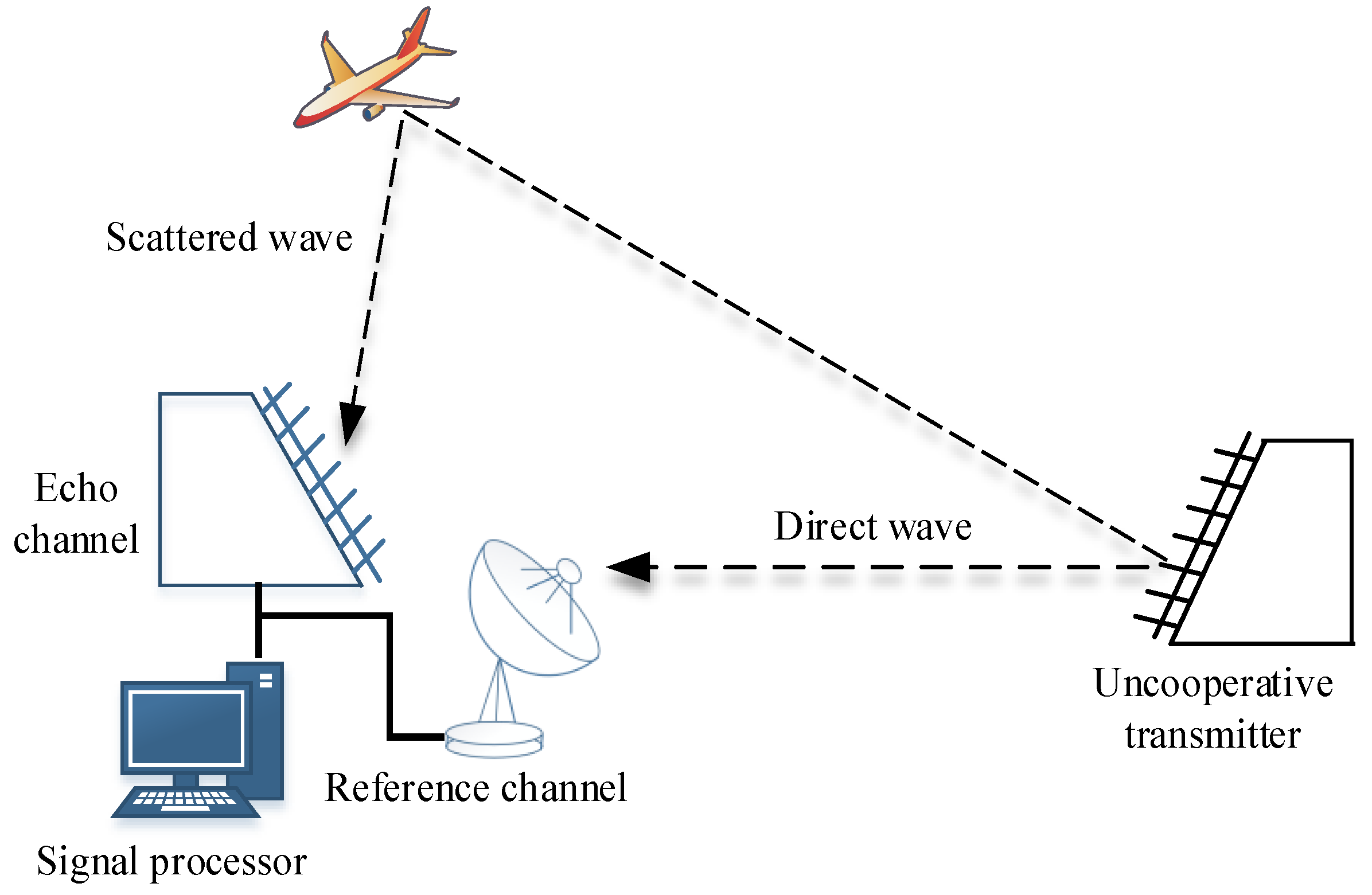
:1. Introduction
- The space synchronization accuracy is not as good as the traditional radar, resulting in the decreased SNR (signal noise ration) and the poor location precision.
- Simultaneous multi-beam forming leads to the redundant data being increased.
- The reference channel is not ideally compatible to the echo channel due to the multipath and the minor difference of antenna performance. The performance of the following pulse compression degrades.
- Due to the agility of the illuminator parameters, the number of the pulses utilized for detection is less. Besides, the scattered wave of the target depends on the opportunity of the beam steering. Thus, the valid data rate is decreased.
- Since the illuminator parameters are agile pulse by pulse, it is hard to adopt coherent integration to suppress clutter like traditional radar.
- Low SNR calls for low threshold during CFAR (constant false alarm), that is to increase the detection rate, whereas the false-alarm rate increases correspondingly.
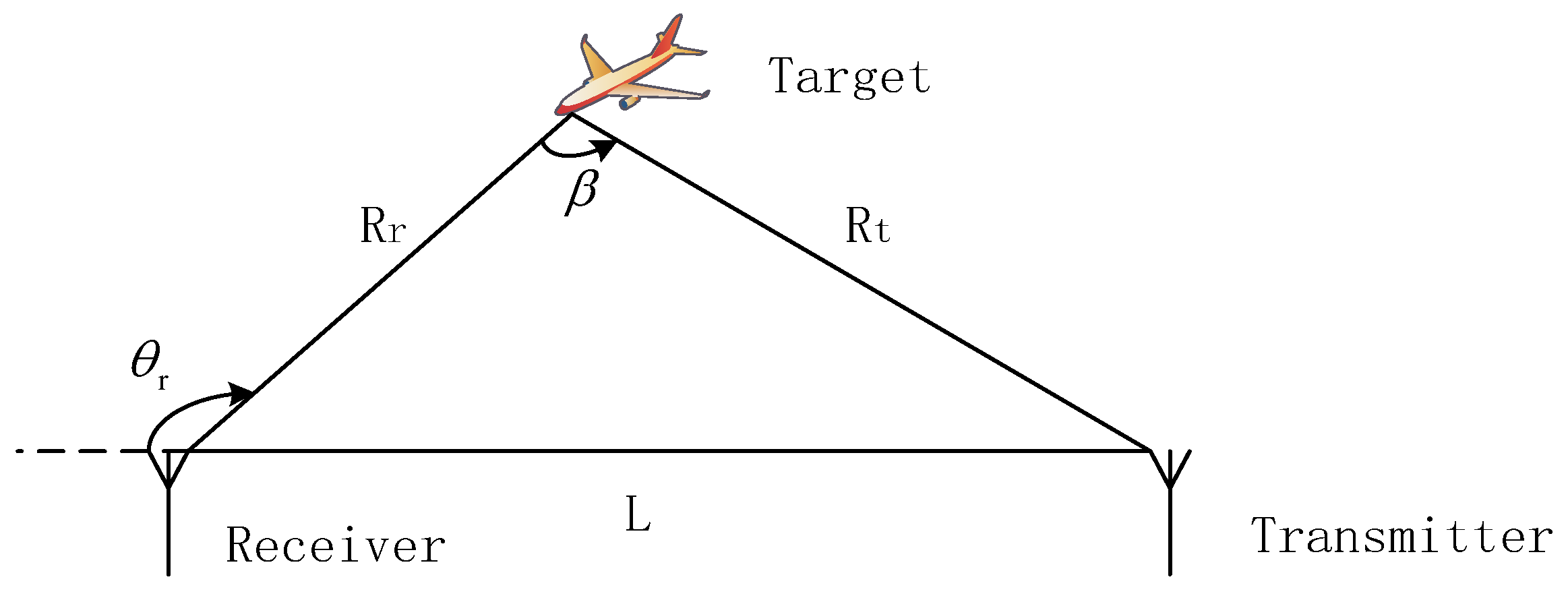
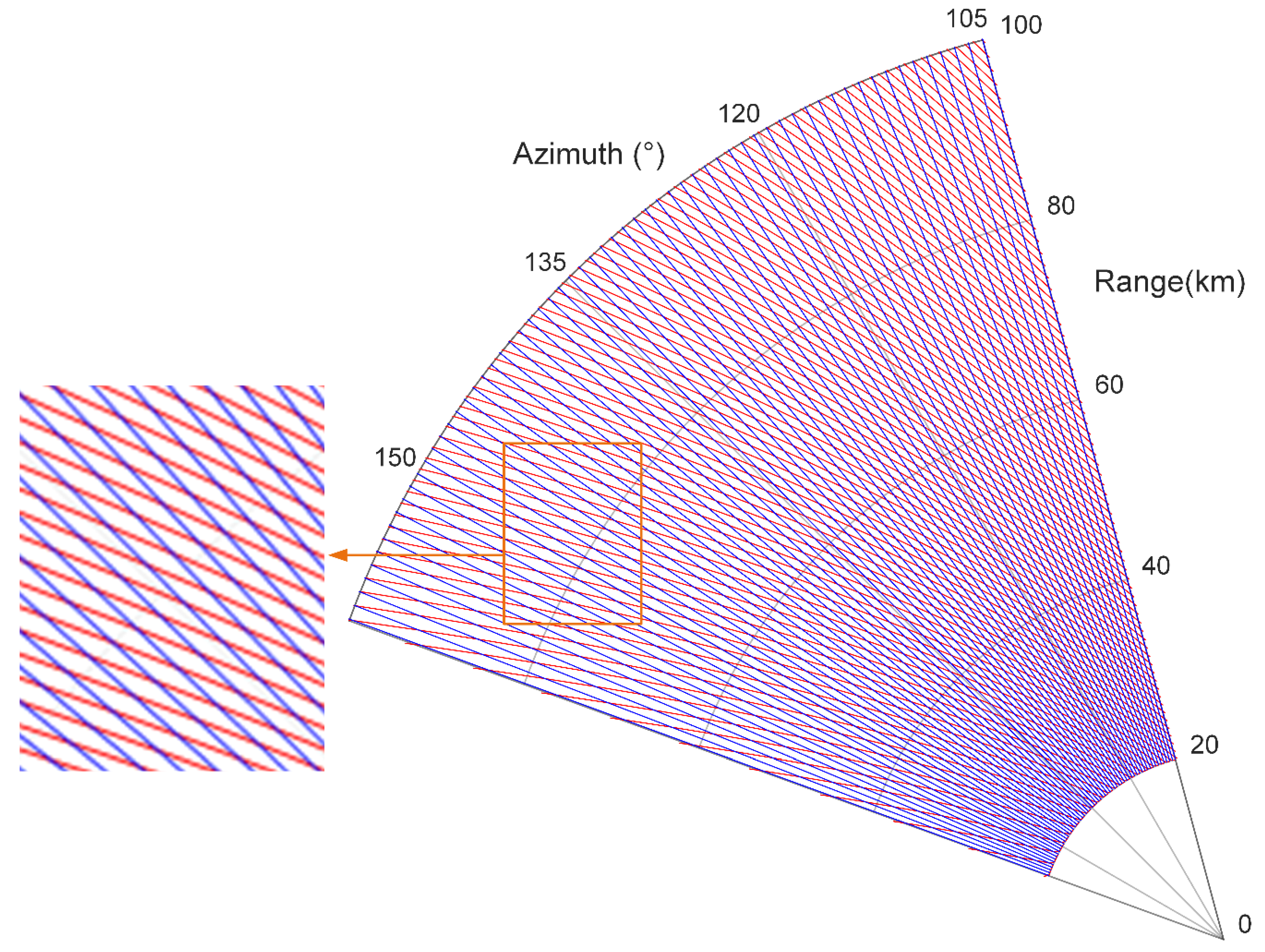
2. Non-Uniform Polar Grid Construction for PBR
3. Separate False Alarm Clutter from Data
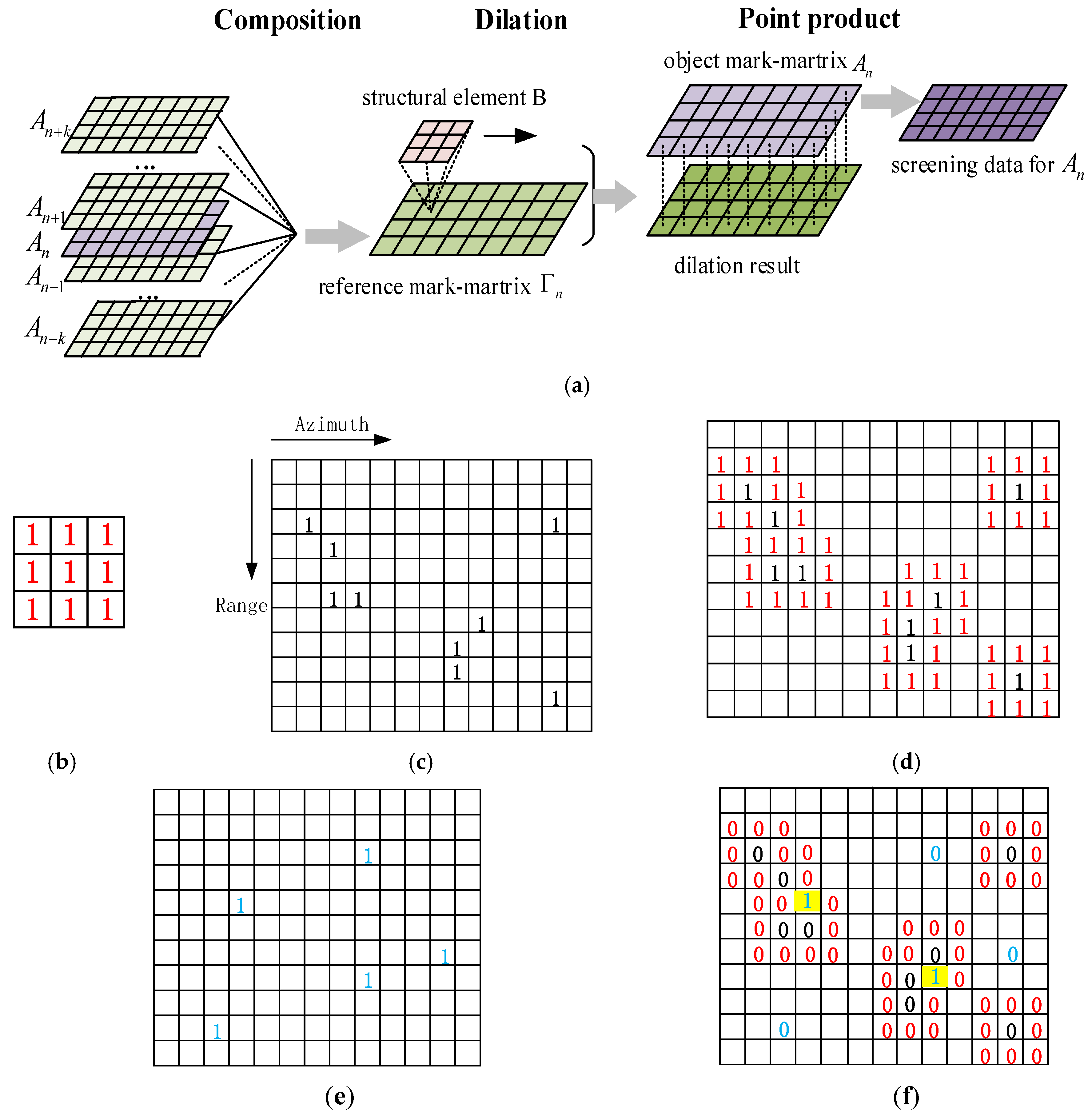
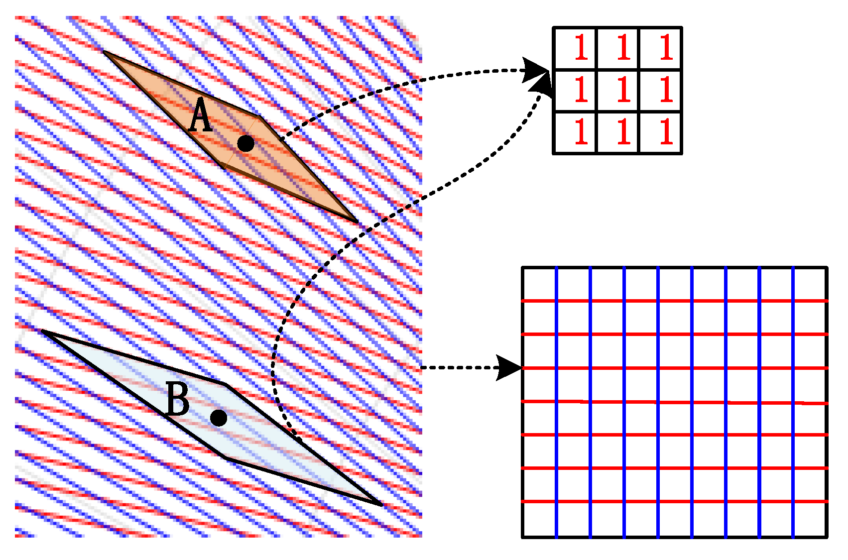
3.1. Mark the Point on Grid
3.2. Separate False Alarm Clutter from Data Based on the Dilation Morphology
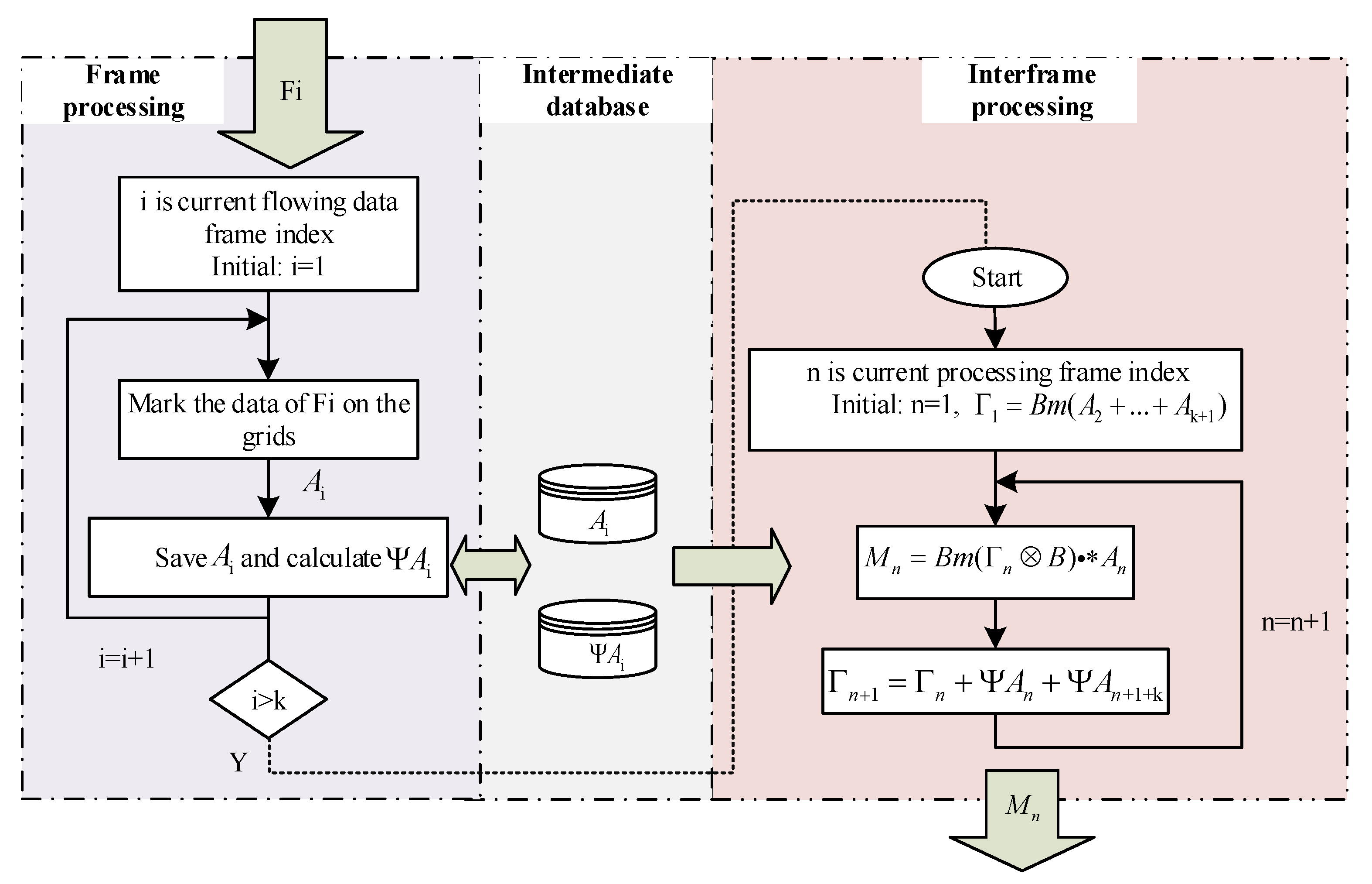
3.3. Iteratively Calculation Frame by Frame
4. Experiment result and Analysis
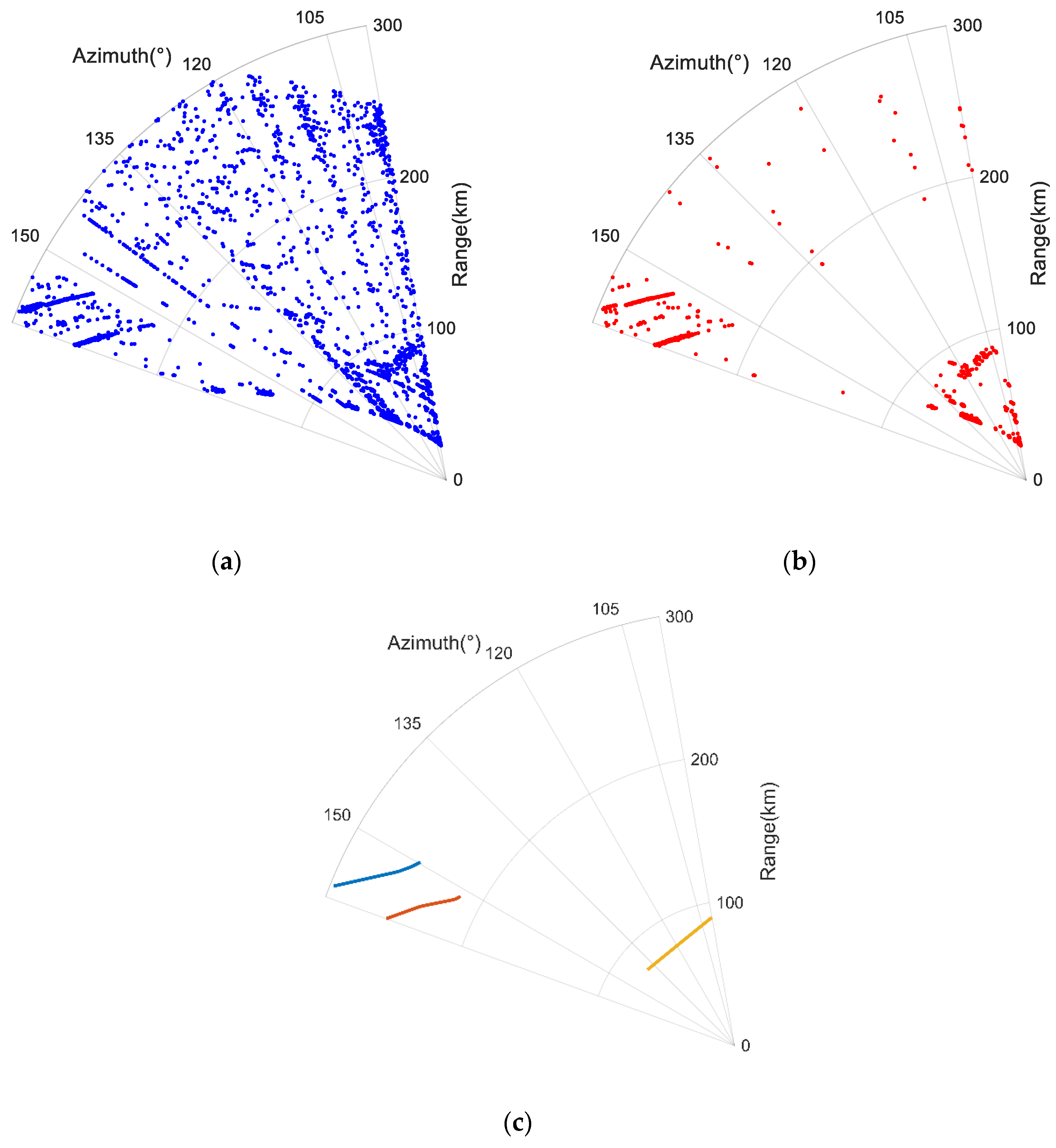
4.1. Testing by Simulated Data
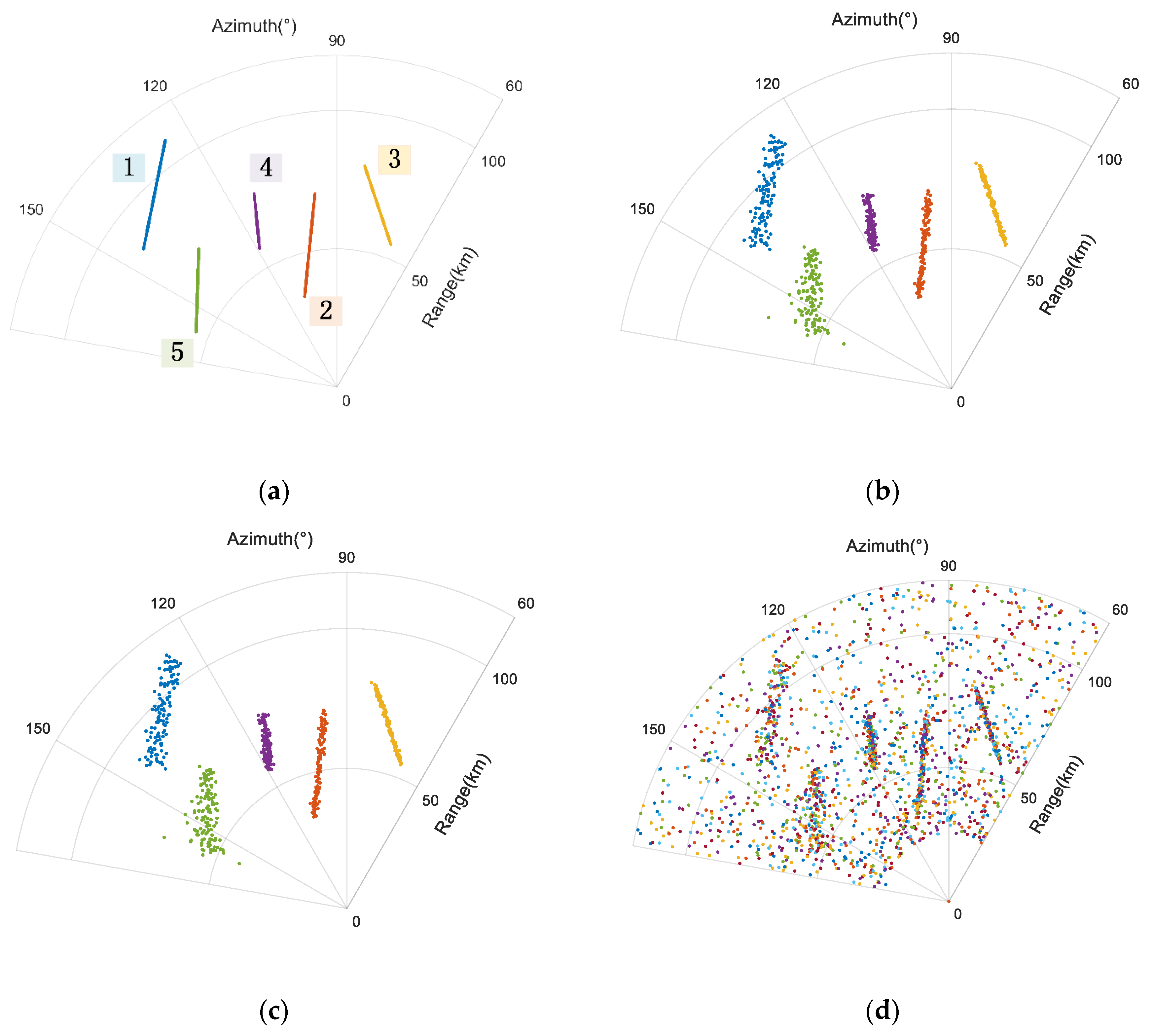
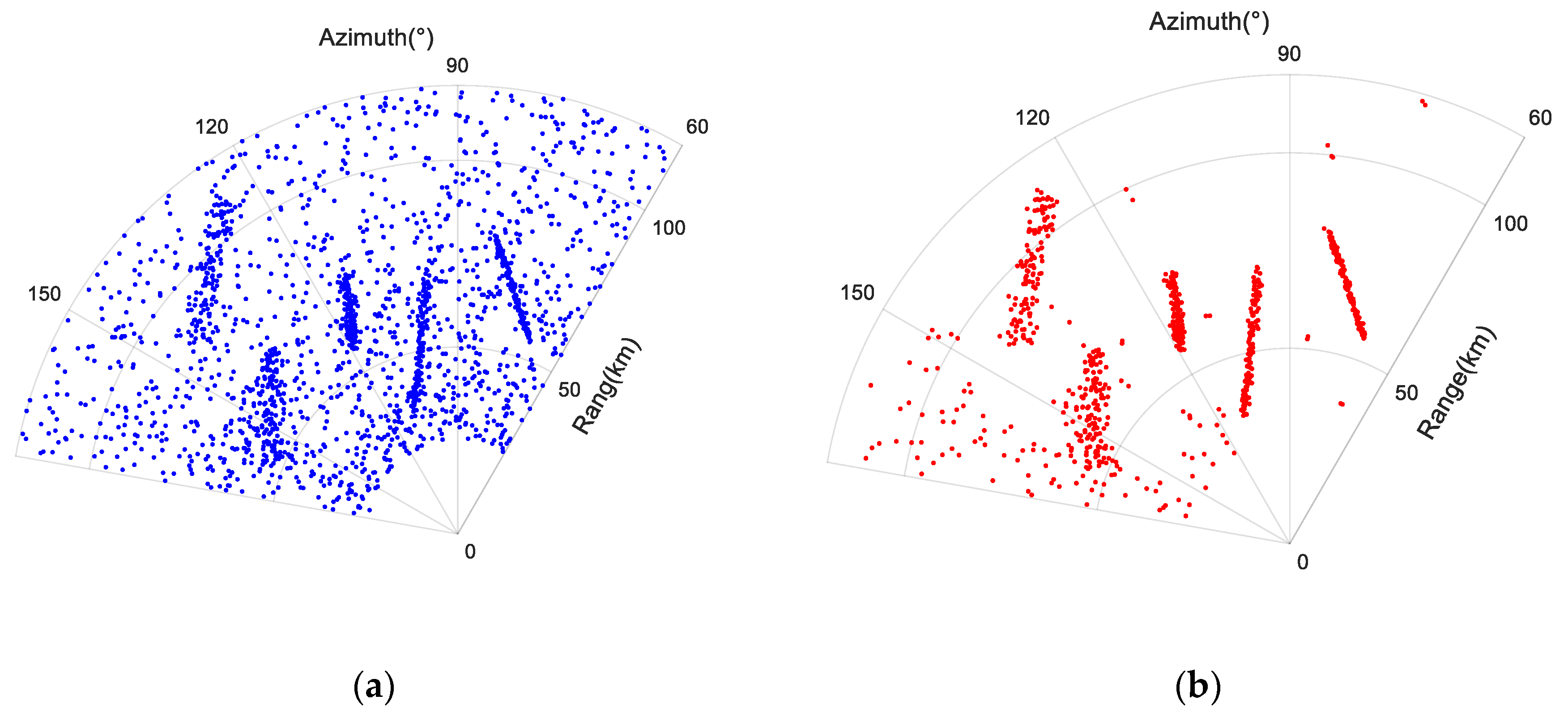
4.1.1. Scenario for Simulation
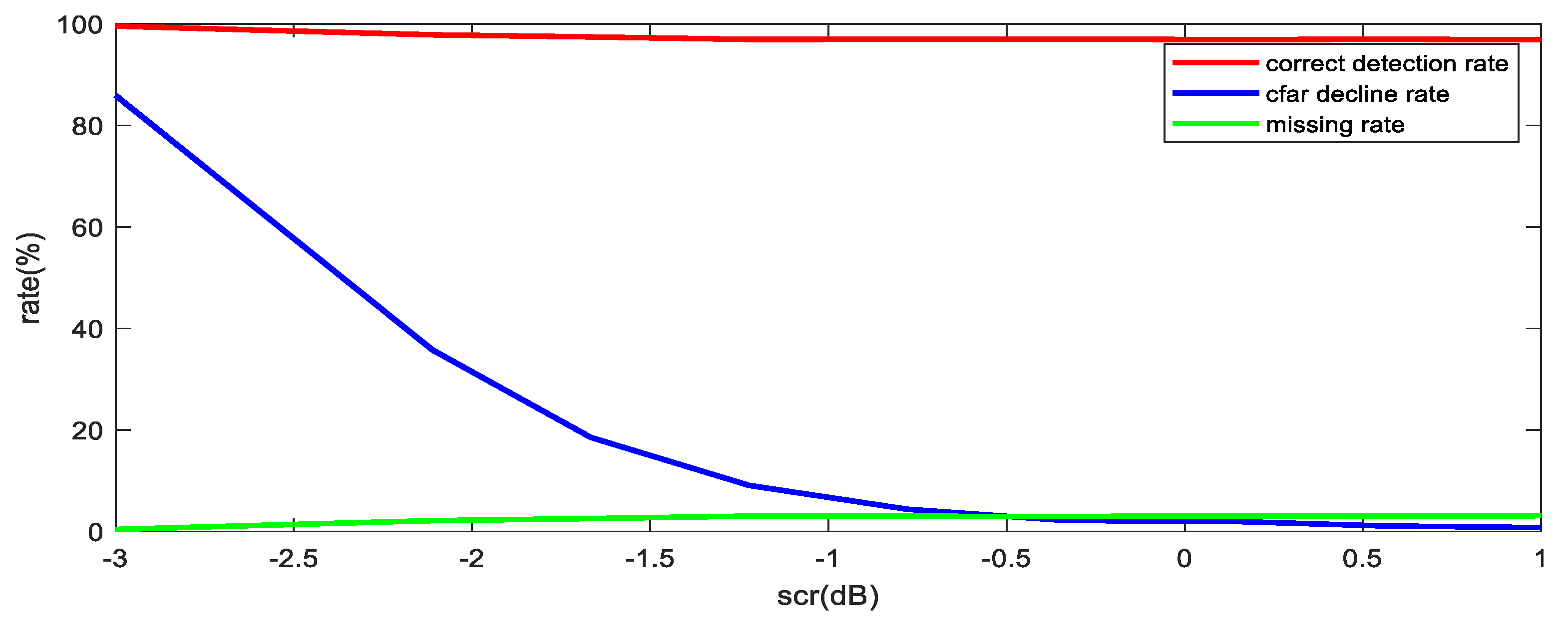
4.1.2. The Clutter Suppression Performance Analysis
4.1.3. Computation Analysis
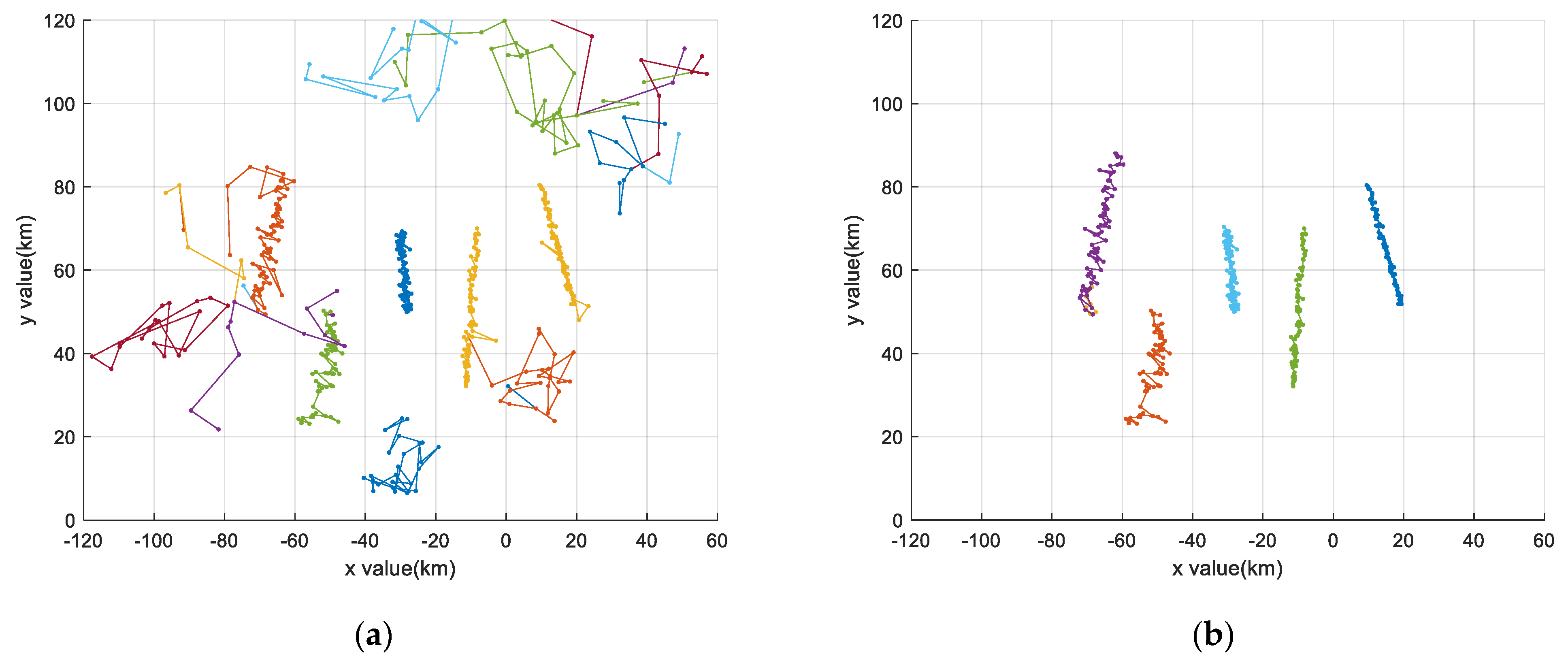
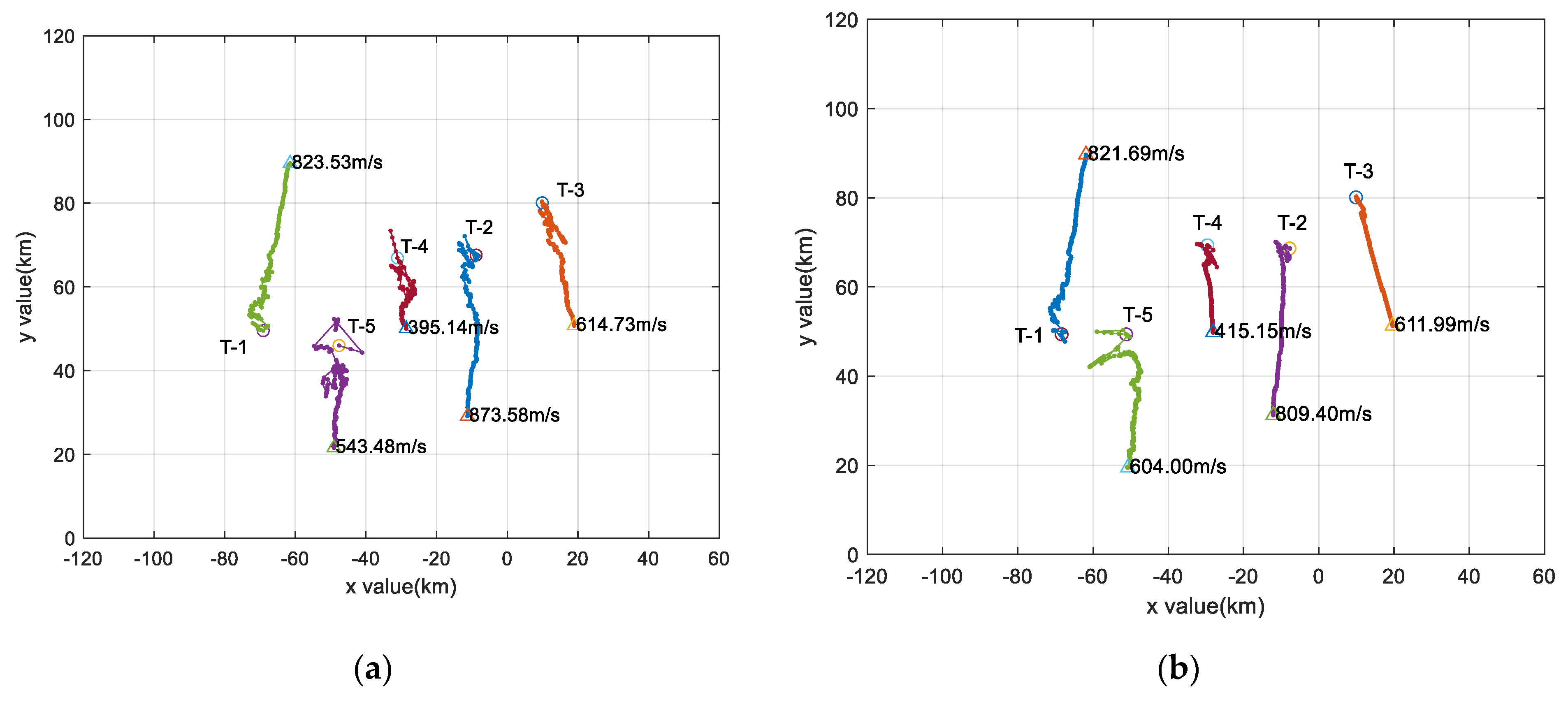
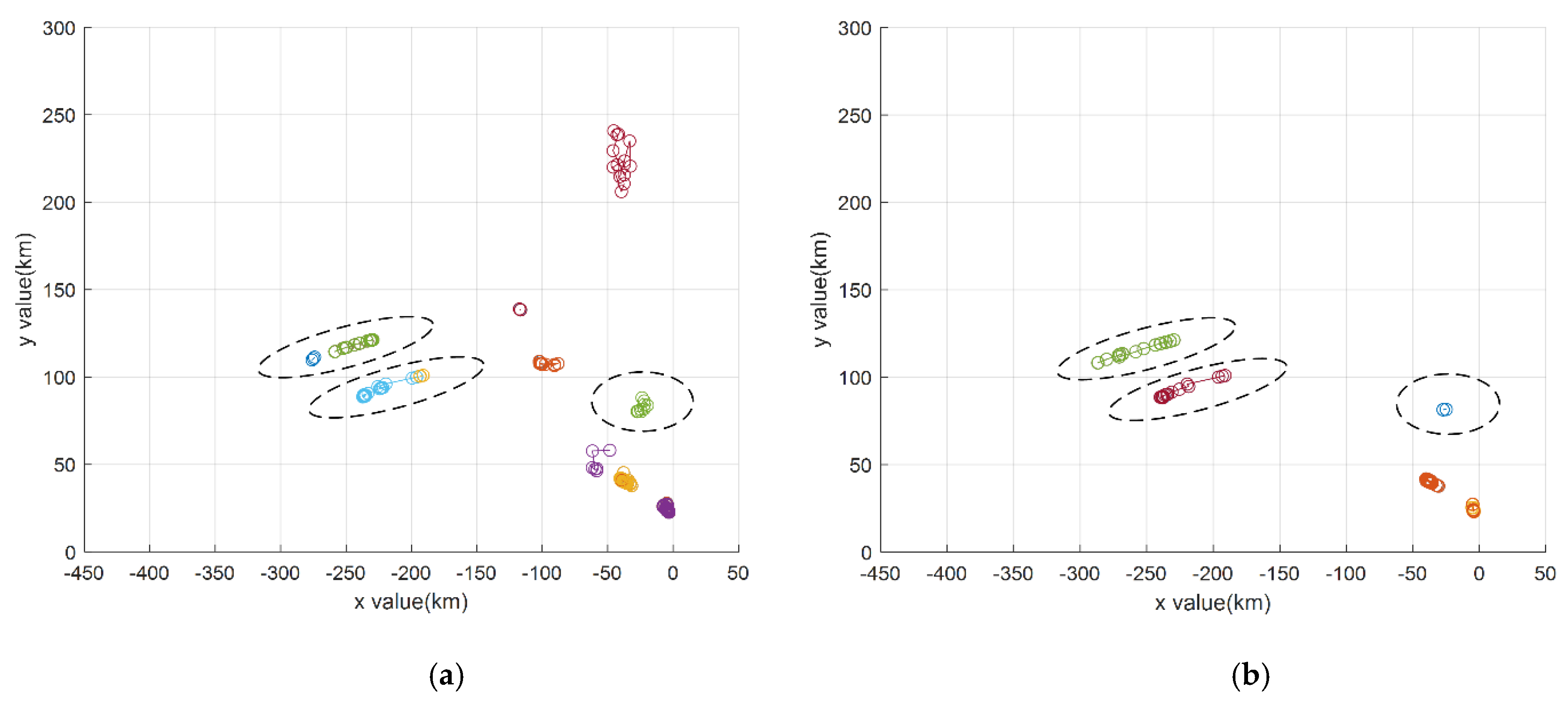
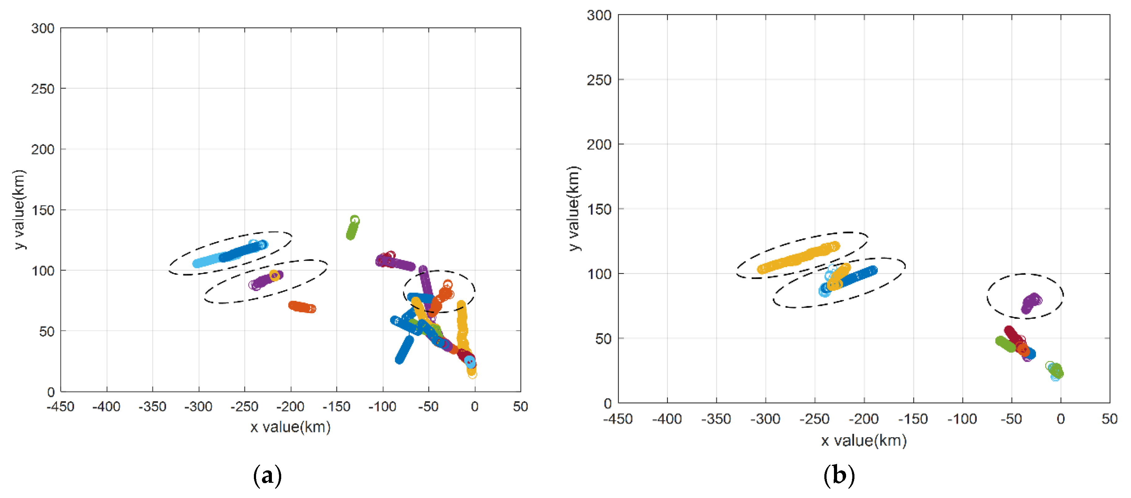
4.1.4. Test the Performance Combining with Tracking Algorithm
4.2. Testing by the Field Data
5. Conclusions
Author Contributions
Funding
Conflicts of Interest
References
- Kuschel, H.; Cristallini, D.; Olsen, K.E. Tutorial: Passive radar tutorial. IEEE Aerosp. Electron. Syst. Mag. 2019, 34, 2–19. [Google Scholar] [CrossRef]
- Zhou, X.; Wang, H.; Cheng, Y.; Qin, Y. Radar coincidence imaging by exploiting the continuity of extended target. IET Radar Sonar Navig. 2017, 11, 60–69. [Google Scholar] [CrossRef]
- Malanowski, M.; Kulpa, K.; Kulpa, J.; Samczynski, P.; Misiurewicz, J. Analysis of detection range of FM-based passive radar. IET Radar Sonar Navig. 2014, 8, 153–159. [Google Scholar] [CrossRef]
- Palmer, J.E.; Harms, H.A.; Searle, S.J.; Davis, L. DVB-T Passive Radar Signal Processing. IEEE Trans. Signal Process. 2013, 61, 2116–2126. [Google Scholar] [CrossRef]
- Pastina, D.; Colone, F.; Martelli, T.; Falcone, P. Parasitic exploitation of wi-fi signals for indoor radar surveillance. IEEE Trans. Veh. Technol 2015, 64, 1401–1415. [Google Scholar] [CrossRef]
- Samczynski, P.; Kulpa, K.; Malanowski, M.; Krysik, P.; Maślikowski, Ł. A concept of GSM-based passive radar for vehicle traffic monitoring. In Proceedings of the Microwaves, Radar and Remote Sensing Symposium, Kiev, Ukraine, 25–27 August 2011; pp. 271–274. [Google Scholar]
- Raja, R.A.; Noor, A.A.; Nur, A.R.; Asem, A.S.; Fazirulhisyam, H. Analysis on target detection and classification in lte based passive forward scattering radar. Sensors 2016, 16, 1607. [Google Scholar] [CrossRef] [PubMed]
- Hong-Cheng, Z.; Jie, C.; Peng-Bo, W.; Wei, Y.; Wei, L. 2-d coherent integration processing and detecting of aircrafts using gnss-based passive radar. Remote Sens. 2018, 10, 1164. [Google Scholar] [CrossRef]
- Ma, H.; Antoniou, M.; Pastina, D.; Santi, F.; Pieralice, F.; Bucciarelli, M.; Cherniakov, M. Maritime Moving Target Indication Using Passive GNSS-based Bistatic Radar. IEEE Trans. Aerosp. Electron. Syst. 2018, 54, 115–130. [Google Scholar] [CrossRef]
- Suberviola, I.; Mayordomo, I.; Mendizabal, J. Experimental results of air target detection with a gps forward-scattering radar. IEEE Geosci. Remote Sens. Lett. 2012, 9, 47–51. [Google Scholar] [CrossRef]
- Wang, Y.; Bao, Q.; Wang, D.; Chen, Z. An experimental study of passive bistatic radar using uncooperative radar as a transmitter. IEEE Geosci. Remote Sens. Lett. 2015, 12, 1–5. [Google Scholar] [CrossRef]
- Zhu, Q.; Bao, Q.; Hu, P.; Chen, Z. Experimental study of aircraft detection by PBR exploiting uncooperative radar as illuminator. In Proceedings of the International Conference on Information, Electronic and Communication Engineering, Beijing, China, 28–29 October 2018; pp. 185–190. [Google Scholar]
- Wang, Y.; Bao, Q.; Chen, Z. Robust adaptive beamforming using IAA-based interference-plus-noise covariance matrix reconstruction. Electron. Lett. 2016, 52, 1185–1186. [Google Scholar] [CrossRef]
- Yang, X.; Xie, J.; Li, H.; He, Z. Robust adaptive beamforming of coherent signals in the presence of the unknown mutual coupling. IET Commun. 2018, 12, 75–81. [Google Scholar] [CrossRef]
- Meller, M. Cheap Cancellation of Strong Echoes for Digital Passive and Noise Radars. IEEE Trans. Signal Process. 2012, 60, 2654–2659. [Google Scholar] [CrossRef]
- Dwivedi, S.; Aggarwal, P.; Jagannatham, A.K. Fast block lms and rls-based parameter estimation and two-dimensional imaging in monostatic mimo radar systems with multiple mobile targets. IEEE Trans. Signal Process. 2018, 66, 1775–1790. [Google Scholar] [CrossRef]
- Guan, X.; Hu, D.H.; Zhong, L.H.; Ding, C.B. Strong echo cancellation based on adaptive block notch filter in passive radar. IEEE Geosci. Remote Sens. Lett. 2015, 12, 339–343. [Google Scholar] [CrossRef]
- Colone, F.; O’Hagan, D.W.; Lombardo, P.; Baker, C.J. A multistage processing algorithm for disturbance removal and target detection in passive bistatic radar. IEEE Trans. Aerosp. Electron. Syst. 2009, 45, 698–722. [Google Scholar] [CrossRef]
- Colone, F.; Palmarini, C.; Martelli, T.; Tilli, E. Sliding extensive cancellation algorithm for disturbance removal in passive radar. IEEE Trans. Aerosp. Electron. Syst. 2016, 52, 1309–1326. [Google Scholar] [CrossRef]
- Fu, Y.; Wan, X.; Zhang, X.; Yi, J.; Zhang, J. Parallel processing algorithm for multipath clutter cancellation in passive radar. IET Radar Sonar Navig. 2018, 12, 121–129. [Google Scholar] [CrossRef]
- Zhao, Z.; Zhou, X.; Zhu, S.; Hong, S. Reduced complexity multipath clutter rejection approach for drm-based hf passive bistatic radar. IEEE Access 2017, 5, 20228–20234. [Google Scholar] [CrossRef]
- Zhao, Z.; Wan, X.; Shao, Q.; Gong, Z.; Cheng, F. Multipath clutter rejection for digital radio mondiale-based HF passive bistatic radar with OFDM waveform. IET Radar Sonar Navig. 2012, 6, 867–872. [Google Scholar] [CrossRef]
- Chabriel, G.; Barrère, J.; Gassier, G.; Briolle, F. Passive Covert Radars using CP-OFDM signals: A new efficient method to extract targets echoes. In Proceedings of the IEEE International Radar Conference, Lille, France, 13–17 October 2014; pp. 1–6. [Google Scholar]
- Kellner, D.; Klappstein, J.; Dietmayer, K. Grid-based dbscan for clustering extended objects in radar data. In Proceedings of the IEEE Intelligent Vehicles Symposium, Madrid, Spain, 3–7 June 2012; pp. 365–370. [Google Scholar]
- Zhang, T.; Mao, X.; Zhao, C.; Liu, J. A novel grid selection method for sky-wave time difference of arrival localization. IET Radar Sonar Navig. 2019, 13, 538–549. [Google Scholar] [CrossRef]
- Guo, J.; Zhang, R. Efficient radar data processing algorithm for dense cluttered environment. In Proceedings of the IEEE Cie International Conference on Radar, Chengdu, China, 24–27 October 2011; pp. 1692–1695. [Google Scholar]
- Pan, S.S. Research and Engineering Realization of Multi-Target Tracking Technology for Non-Cooperative Passive Detection System. Master’s Thesis, National University of Defense Technology, Changsha, China, 2017. [Google Scholar]


| 1. Calculate angular coordinate |
| The angular coordinate set is . Where is the symbol of round down, and N is the mesh counts in angular dimension. |
| 2. Aiming at each angular coordinate in Θ, iteratively calculate the grid division in range dimension. |
| For , Initialization: , = ; Iteration: ; , . ; Terminate when . . is the mesh counts in range dimension for . The range coordinate set is . |
| Start Position (km, degree) in Polar Coordinates | Start Position (km) in Cartesian Coordinates | Track Slope | Track Intercept (km) | |
|---|---|---|---|---|
| Target 1 | (86.023,144.5) | (−70, 50) | 5 | 60 |
| Target 2 | (70.456,96.5) | (−8, 70) | 10 | 100 |
| Target 3 | (80.623,82.9) | (10, 80) | −3 | 10 |
| Target 4 | (76.158,113.2) | (−30, 70) | −10 | 80 |
| Target 5 | (70.711,135) | (−50, 50) | 30 | 55 |
| Detection Accuracy Rate | False Alarm Decline Rate | Miss Detection Rate |
|---|---|---|
| 97.45% | 10.24% | 2.55% |
| Total Number of Traces | Mean Trace Length | Max Trace Length | Time Consuming (s) | |
|---|---|---|---|---|
| NN-MHT | 22 | 39.13 | 89 | 2.99 |
| MCSNG-NN | 6 | 78.83 | 89 | 0.7 |
| Mean Trace Error (m) | Velocity (m/s) | ||||
|---|---|---|---|---|---|
| Track NO. | SNN-Kalman | MCSNG-SNN-K | SNN-Kalman | MCSNG-SNN-K | True Value |
| 1 | 548.87 | 434.56 | 823.5 | 821.7 | 800 |
| 2 | 1596.55 | 389.63 | 873.6 | 809.4 | 750 |
| 3 | 644.06 | 141.85 | 614.7 | 612.0 | 600 |
| 4 | 1286.59 | 283.97 | 395.1 | 415.2 | 400 |
| 5 | 2721.07 | 1840.33 | 543.5 | 604.0 | 600 |
| Total Number of Traces | Mean Trace Length | Max Trace Length | Time Consuming (s) | |
|---|---|---|---|---|
| SNN-Kalman | 104 | 64.89 | 654 | 0.6715 |
| MCSNG-SNN-K | 23 | 124.47 | 474 | 0.6081 |
| Total Number of Traces | Mean Trace Length | Max Trace Length | Time Consuming (s) | |
|---|---|---|---|---|
| NN-MHT | 31 | 38.7 | 135 | 4.83 |
| MCSNG-NN | 9 | 39.3 | 120 | 1.36 |
| Total Number of Traces | Mean Trace Length | Max Trace Length | Time Consuming (s) | |
|---|---|---|---|---|
| SNN-Kalman | 23 | 254.5 | 734 | 0.8536 |
| MCSNG-SNN-K | 13 | 196.6 | 424 | 0.6467 |
© 2019 by the authors. Licensee MDPI, Basel, Switzerland. This article is an open access article distributed under the terms and conditions of the Creative Commons Attribution (CC BY) license (http://creativecommons.org/licenses/by/4.0/).
Share and Cite
Zhu, Q.; Li, T.; Pan, J.; Bao, Q. PBR Clutter Suppression Algorithm Based on Dilation Morphology of Non-Uniform Grid. Electronics 2019, 8, 708. https://doi.org/10.3390/electronics8060708
Zhu Q, Li T, Pan J, Bao Q. PBR Clutter Suppression Algorithm Based on Dilation Morphology of Non-Uniform Grid. Electronics. 2019; 8(6):708. https://doi.org/10.3390/electronics8060708
Chicago/Turabian StyleZhu, Qian, Tao Li, Jiameng Pan, and Qinglong Bao. 2019. "PBR Clutter Suppression Algorithm Based on Dilation Morphology of Non-Uniform Grid" Electronics 8, no. 6: 708. https://doi.org/10.3390/electronics8060708