Effect of Sensors Sensitivity on Lithium-Ion Battery Modeled Parameters and State of Charge: A Comparative Study

Abstract

The accurate estimation of the state of charge (SOC) is usually acknowledged as one of the essential features in designing of battery management system (BMS) for the lithium-ion batteries (LIBs) in electric vehicles (EVs). A suitable battery model is a prerequisite for correct SOC measurement. In this work, the first and second order RC autoregressive exogenous (ARX) battery models are adopted to check the influence of voltage and current transducer measurement uncertainty. The Lagrange multiplier method is used to estimate the battery parameters. The sensitivity analysis is performed under the following conditions: Current sensor precision of ±5 mA, ±50 mA, ±100 mA, and ±500 mA and voltage sensor precision of ±1 mV, ±2.5 mV, ±5 mV, and ±10mV. The comparative analysis of both models under the perturbed environment has been carried out. The effects of the sensor’s sensitivity on the different battery structures and complexity are also analyzed. Results shows that the voltage and current sensor sensitivity has a significant influence on SOC estimation. This research outcome assists the researcher in selecting the optimal value of sensor accuracy to accurately estimate the SOC of the LIB.

1. Introduction

Due to escalation in environmental pollution and energy prices, electric vehicles (EVs) have been widely explored in the past few years. Battery electric vehicles (BEVs), plug-in hybrid electric vehicles (PHEVs), and fuel cell electric vehicles (FCEVs) are the different variants of EVs [1]. According to a report [2], the annual sale of EVs is anticipated to be almost 100 million at the end of the year 2050. These EVs consist of energy storage and the motor system as the secondary or main energy source (FCEVs and PHEVs) or the sole energy source (BEVs) [3]. Sodium sulphur (NaS) batteries, sodium nickel chloride (NaNiCl), vanadium redox flow batteries (VRFB), zinc bromine flow batteries (ZBFB), lead-acid batteries, lithium-ion batteries (LIBs), and nickel metal hydride batteries (NiMH) can be used as an energy storage system (ESS) in EVs [4,5]. The LIBs have the most promising features like high energy and power density, lightweight, low self-discharge rate, long life span, and better efficiency as compared to others [5]. The LIB is not only the weightiest onboard ESS for EVs [6,7] but also an integral part of the smart grid [8,9]. An advanced battery management system (BMS) is needed to ensure safe, reliable, and efficient operation of LIB in EVs, which can measure/estimate state of charge (SOC), state of health (SOH), and state of power (SOP) with high accuracy [10,11].

Assortments of methodologies can be found in the literature to estimate the SOC of the LIB. Each methodology has its own supremacy and lapses [10]. In model-based techniques, the identification of model parameters and SOC estimation are key indicators in a BMS to protect the LIB. The SOC estimation accuracy mainly relies on the operational conditions, battery aging, modeling error, and measurement uncertainty. He et al. [12] proposed an improved second order RC model to tackle the effects of different charging and discharging rates on the cell capacity. They used an adaptive extended Kalman filter (AEKF) to estimate the SOC. The Lagrange multiplier method was adopted to find the parameters of battery model under different current variations [13]. In other studies [14,15,16], the effects of temperature variation have been considered to develop a temperature compensated model to estimate the SOC of LIB. Wang et al. [17] proposed a joint estimator to measure the SOC and available energy of LIB. They jointly considered the effects of temperature and different charge/discharge rates to estimate the states using particle filter (PF). In [18], the authors implemented the unscented Kalman filter (UKF) with an improved battery model to observe the effects of temperature variation and charge/discharge rate. Zheng et al. [19] considered the effect of battery aging to estimate the SOC accurately. The experimental results show the accuracy of their proposed methodology. Chaoui et al. [20] proposed a time-delayed neural network method to estimate the SOC and SOH of the LIB. Battery temperature, voltage, and current values were the input of the estimator. Their presented methodology compensated the nonlinear battery degradation due to aging. Xiong et al. [21] proposed a battery model against different aging level of batteries. Their experimental results show the effectiveness and accuracy of the proposed model at different aging levels at 1 s sampling time. The estimation error of their proposed approach was less than 2%. In [22], the authors thoroughly investigate the different sources of errors in online SOC estimation methods.

The effects of sensor sensitivity on the modeling parameters and SOC estimation remain an emerging research area. A temperature-compensated battery model was developed to find the parameters at different temperatures [23]. A dual PF was proposed to estimate the SOC and drift current to eliminate the drift-noise error. They added a static parameter in a temperature-compensated model to address the issue of drift current. The results reveal that their proposed model has maximum errors of 2.83% and 5.11% at 0.15% current drift and 45 °C respectively. In [24], a nonlinear observer to estimate the SOC of LIB was designed, and it shows that the estimation error did not exceed 4.5% in the presence of voltage and current sensor errors of 2.5% and 5% respectively.

The measuring current/voltage sensor error can be divided into two groups: Fixed errors and random errors. The fixed error is a static value which can add into measured value at any given time. This error can be tackled easily by calibrating the resultant measured value. A random error primarily induced by the resolution of voltage/current sensors [25]. Lai et al. [26] compared different equivalent circuit models for estimating the SOC. They added fixed voltage and current drift error to analyze the effects on SOC estimation. The increase of 35.5% and 37.8% in estimation error was observed at 0.1 A uncertainty in first and second order battery models respectively. The effects of sensor error and sampling time on states estimation of LIB was studied in [27]. The authors used a first order RC circuit in their work. The maximum noted estimation error was 1.72% at 0.1 s sampling time.

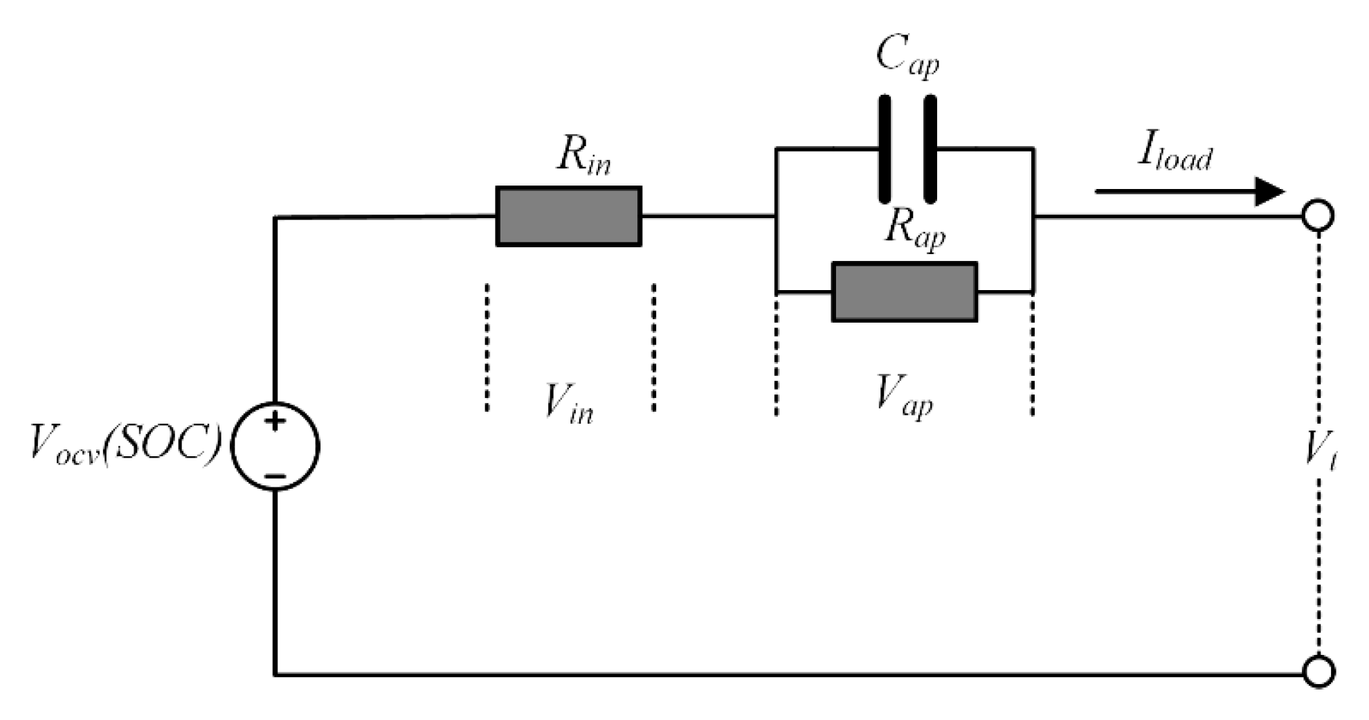
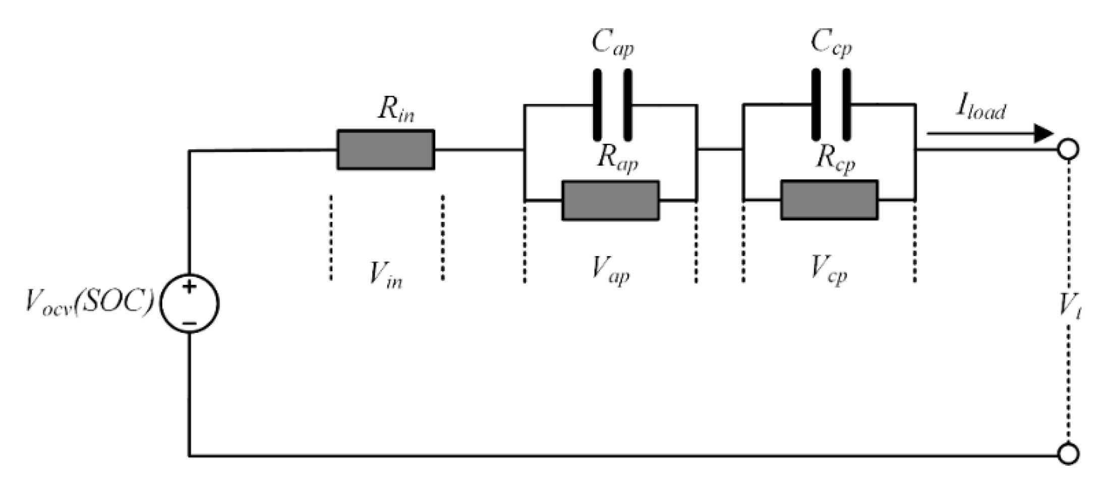
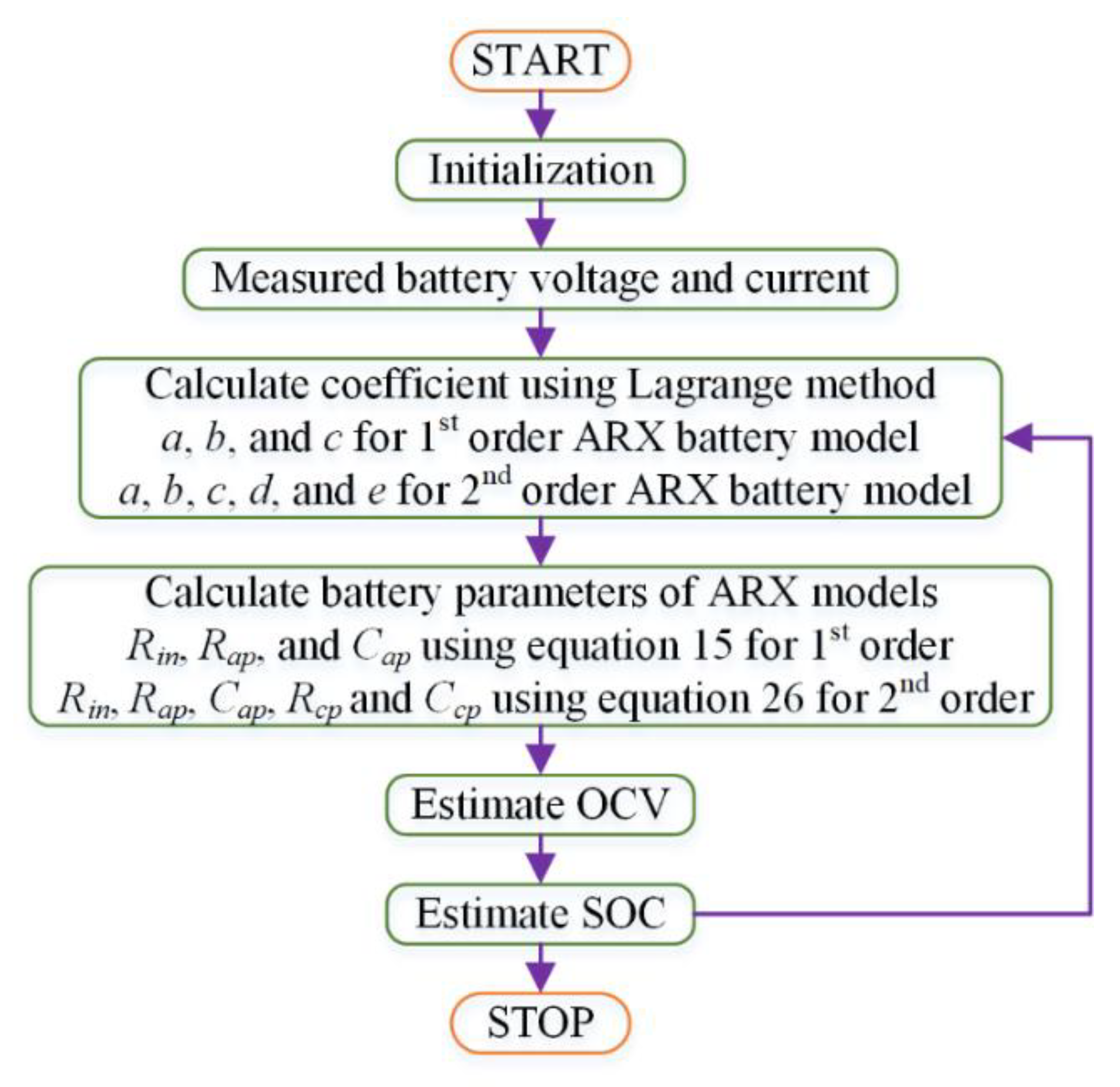
In this paper, the sensor sensitivity analysis is evaluated to observe the sensor precision effects on identified battery model parameters and estimated SOC. The experiment is performed to determine the OCV-SOC relationship. The Lagrange multiplier method is adopted to determine the online battery parameters and SOC of the first and second order RC autoregressive exogenous (ARX) battery model. The sensitivity analysis is carried out for these scenarios: Current sensor precision of ±5 mA, ±50 mA, ±100 mA, and ±500 mA and voltage sensor precision of ±1 mV, ±2.5 mV, ±5 mV, and ±10 mV. The comparative analysis of the models under the perturbed environment has been carried out to draw some insightful results.

2. Autoregressive Exogenous (ARX) Battery Models and Parameter Identification Technique

This section explains the two different ARX battery model and their associated parameters estimation methodology. In this work, first order and second order RC models have been selected owing to their high accuracy and reliability for LIB [26].

2.1. Battery Models

2.1.1. First Order ARX Battery Model

Figure 1 shows the schematic diagram of the first order RC model [28]. The battery model consists of battery open circuit voltage $V_{ocv}\left(SOC\right)$, battery internal resistance $R_{in}$, electrochemical diffusion resistance $R_{ap}$, and electrochemical diffusion capacitance $C_{ap}.$ The parallel $R_{ap}{C}_{ap}$ network modeled the transient behavior of the battery. $V_{in}$ and $V_{ap}$ denote the voltage drop across $R_{in}$ and $R_{ap}{C}_{ap}$, respectively. $I_{load}$ and $V_t$ are the charge/discharge current and terminal voltage of the battery.

According to the first order ARX battery model, the electrical behavior of the battery in mathematical form can be expressed as follows [29]:

$$V_{ocv}\left(SOC\right)=\begin{array}{c}{V}_t+V_{in}+V_{ap}\\ V_t+I_{load}{R}_{in}+V_{ap}\end{array}\}$$

(1)

$$\dot{V_{ap}}=-\frac{1}{R_{ap}{C}_{ap}}{V}_{ap}+\frac{1}{C_{ap}}{I}_{load}$$

(2)

2.1.2. Second Order ARX Battery Model

Figure 2 shows the schematic diagram of the second order RC model [30]. The battery model consists of battery open circuit voltage $V_{ocv}\left(SOC\right)$, battery internal resistance $R_{in}$, electrochemical diffusion resistance $R_{ap}$, electrochemical diffusion capacitance $C_{ap}$, concentration polarization resistance $R_{cp}$, and concentration polarization capacitance $C_{cp}$. The combination of parallel $R_{ap}{C}_{ap}$ and $R_{cp}{C}_{cp}$ network modeled the transient behavior of the battery. $V_{in}$, $V_{ap}$, and $V_{cp}$ denote the voltage drop across $R_{in}$, $R_{ap}{C}_{ap}$, and $R_{cp}{C}_{cp}$ respectively. $I_{load}$ and $V_t$ are the charge/discharge current and terminal voltage of the battery.

According to second order ARX battery model, the electrical behavior of the battery in mathematical form can be expressed as follows [29]:

$$V_{ocv}\left(SOC\right)=\begin{array}{l}{V}_t+V_{in}+V_{ap}+V_{cp}\hfill \\ V_t+I_{load}{R}_{in}+V_{ap}+V_{cp}\hfill \end{array}\}$$

(3)

$$\dot{V_{ap}}=-\frac{1}{R_{ap}{C}_{ap}}{V}_{ap}+\frac{1}{C_{ap}}{I}_{load}$$

(4)

$$\dot{V_{cp}}=-\frac{1}{R_{cp}{C}_{cp}}{V}_{cp}+\frac{1}{C_{cp}}{I}_{load}$$

(5)

2.2. Lagrange Multiplier Method for Parameter Estimation

2.2.1. First Order ARX Battery Model

By applying the Laplace transform to Equations (1) and (2), the frequency domain model of the first order ARX battery model can be written as:

$$V_t=V_{ocv}\left(SOC\right)-I_{load}\left(s\right)R_{in}-I_{load}\left(s\right)\frac{R_{ap}}{1+R_{ap}{C}_{ap}s}$$

(6)

Defining $V_{ocv}\left(SOC\right)-V_t=V_b$ in Equation (6), the transfer function of the model can be written as:

$$G\left(s\right)=\frac{V_b\left(s\right)}{I_{load}\left(s\right)}=\frac{R_{in}+R_{ap}+R_{in}{R}_{ap}{C}_{ap}s}{1+R_{ap}{C}_{ap}s}$$

(7)

By applying bilinear transformation $s=2\left(z-1\right)/T_s\left(z+1\right)$ in the above Equation, the first order ARX battery model can be discretized as:

$$G\left(z^{-1}\right)=\frac{V_b\left(z^{-1}\right)}{I_{load}\left(z^{-1}\right)}=\frac{a+b{z}^{-1}}{1+c{z}^{-1}}$$

(8)

By applying inverse z-transform, the frequency domain battery model can be converted to time domain discrete battery model as:

$$\begin{array}{c}{V}_b\left(k+1\right)=c{V}_b\left(k\right)+a{I}_{load}\left(k+1\right)+b{I}_{load}\left(k\right)\\ V_{ocv}\left(SOC\right)\left(k+1\right)-V_t\left(k+1\right)=c(V_{ocv}\left(SOC\right)\left(k+1\right)-V_t\left(k+1\right))+a{I}_{load}\left(k+1\right)+b{I}_{load}\left(k\right)\end{array}$$

(9)

where $k$ is the discrete time points and its value are $k=0,1,2,3,\dots ,N$ seconds.

Now defining

$$\begin{array}{l}{V}_b\left(k+j\right)=y\left(k+j\right);forj=1,2,3,\dots ,N\hfill \\ V_b\left(k+j\right)=x_a\left(k+j+1\right);forj=0,1,2,\dots ,N\hfill \\ I_{load}\left(k+j\right)=x_b\left(k+j\right);forj=1,2,3,\dots ,N\hfill \\ I_{load}\left(k+j\right)=x_c\left(k+j+1\right);forj=0,1,2,\dots ,N\hfill \end{array}\}$$

(10)

Suppose

$$\left[\begin{array}{c}y\left(k+1\right)\\ \begin{array}{c}y\left(k+2\right)\\ \begin{array}{c}⋮\\ y\left(k+N\right)\end{array}\end{array}\end{array}\right]=\left[\begin{array}{c}\begin{array}{cc}{x}_a\left(k+1\right)& \begin{array}{cc}{x}_b\left(k+1\right)& x_c\left(k+1\right)\end{array}\end{array}\\ \begin{array}{c}\begin{array}{cc}{x}_a\left(k+2\right)& \begin{array}{cc}{x}_b\left(k+2\right)& x_c\left(k+2\right)\end{array}\end{array}\\ \begin{array}{c}\begin{array}{ccc}⋮& ⋮& ⋮\end{array}\\ \begin{array}{cc}{x}_a\left(k+N\right)& \begin{array}{cc}{x}_b\left(k+N\right)& x_c\left(k+N\right)\end{array}\end{array}\end{array}\end{array}\end{array}\right]\left[\begin{array}{c}c\\ \begin{array}{c}a\\ b\end{array}\end{array}\right]$$

(11)

or

$$y\left(k\right)=\mathrm{X}\left(k\right)A$$

(12)

where

$$x\left(k+j\right)=\left[\begin{array}{c}{x}_a\left(k+j\right)\\ x_b\left(k+j\right)\\ x_c\left(k+j\right)\end{array}\right]\forall j=1,2,3,\dots ,N.$$

(13)

$$A=\left[\begin{array}{c}c\\ \begin{array}{c}a\\ b\end{array}\end{array}\right]$$

(14)

These variables $a$, $b$, and $c$ can be identified using the Lagrange multiplier method reported in [13]. The Lagrange multiplier method is adopted due to low computational complexity, better convergence time, and high accuracy. After identifying the values, the battery parameters of the first order RC model can be calculated by using the following formulas.

$$\begin{array}{l}{R}_{in}=\frac{a-b}{1-c}\hfill \\ R_{ap}=\frac{2\left(ca+b\right)}{1-c^2}\hfill \\ C_{ap}=\frac{T{\left(1+c\right)}^2}{4\left(ca+b\right)}\hfill \end{array}\}$$

(15)

2.2.2. Second Order ARX Battery Model

By applying the Laplace transform to Equations (3)–(5), the frequency domain model of the second order ARX battery model can be written as:

$$V_t=V_{ocv}\left(SOC\right)-I_{load}\left(s\right)R_{in}-I_{load}\left(s\right)\frac{R_{ap}}{1+R_{ap}{C}_{ap}s}-I_{load}\left(s\right)\frac{R_{cp}}{R_{cp}{C}_{cp}s}$$

(16)

Putting $V_{ocv}\left(SOC\right)-V_t=V_b$ in Equation (16), the transfer function of the model can be written as:

$$G\left(s\right)=\frac{V_b\left(s\right)}{I_{load}\left(s\right)}=R_{in}+\frac{R_{ap}}{R_{ap}{C}_{ap}s}+\frac{R_{cp}}{R_{cp}{C}_{cp}s}$$

(17)

Put $R_{ap}{C}_{ap}={\tau }_{ap}$ and $R_{cp}{C}_{cp}={\tau }_{cp}$ in Equation (17), it becomes

$$G\left(s\right)=\frac{V_b\left(s\right)}{I_{load}\left(s\right)}=\frac{R_{in}{s}^2+\frac{R_{in}\left({\tau }_{ap}+{\tau }_{cp}\right)+R_{ap}{\tau }_{cp}+R_{cp}{\tau }_{ap}}{{\tau }_{ap}{\tau }_{cp}}s+\frac{R_{in}+R_{ap}{R}_{cp}}{{\tau }_{ap}{\tau }_{cp}}}{s^2+\frac{{\tau }_{ap}+{\tau }_{cp}}{{\tau }_{ap}{\tau }_{cp}}s+\frac{1}{{\tau }_{ap}{\tau }_{cp}}}$$

(18)

By applying bilinear transformation $s=2\left(z-1\right)/T_s\left(z+1\right)$ in the above equation, the second order ARX battery model can be discretized as:

$$G\left(z^{-1}\right)=\frac{V_b\left(z^{-1}\right)}{I_{load}\left(z^{-1}\right)}=\frac{a+b{z}^{-1}+c{z}^{-2}}{1-d{z}^{-1}-e{z}^{-2}}$$

(19)

By applying inverse z-transform, the frequency domain battery model can be converted to time domain discrete battery model as:

$$V_b\left(k+1\right)=d{V}_b\left(k\right)+e{V}_b\left(k-1\right)+a{I}_{load}\left(k+1\right)+b{I}_{load}\left(k\right)+c{I}_{load}\left(k-1\right)$$

(20)

where $k$ is the discrete time points and its values are $k=0,1,2,3,\dots ,N$ seconds.

Now defining

$$\begin{array}{l}{V}_b\left(k+j\right)=y\left(k+j\right);forj=1,2,3,\dots ,N\hfill \\ V_b\left(k+j\right)=x_a\left(k+j+1\right);forj=0,1,2,\dots ,N\hfill \\ V_b\left(k+j-1\right)=x_b\left(k+j+1\right);forj=0,1,2,\dots ,N\hfill \\ I_{load}\left(k+j\right)=x_c\left(k+j\right);forj=1,2,3,\dots ,N\hfill \\ I_{load}\left(k+j\right)=x_d\left(k+j+1\right);forj=0,1,2,\dots ,N\hfill \\ I_{load}\left(k+j-1\right)=x_e\left(k+j+1\right);forj=0,1,2,\dots ,N\hfill \end{array}\}$$

(21)

Suppose

$$\left[\begin{array}{c}y\left(k+1\right)\\ \begin{array}{c}y\left(k+2\right)\\ \begin{array}{c}⋮\\ y\left(k+N\right)\end{array}\end{array}\end{array}\right]=\left[\begin{array}{ccccc}{x}_a\left(k+1\right)& x_b\left(k+1\right)& x_c\left(k+1\right)& x_d\left(k+1\right)& x_e\left(k+1\right)\\ x_a\left(k+2\right)& x_b\left(k+2\right)& x_c\left(k+2\right)& x_d\left(k+2\right)& x_e\left(k+2\right)\\ ⋮& ⋮& ⋮& ⋮& ⋮\\ x_a\left(k+N\right)& x_b\left(k+N\right)& x_c\left(k+N\right)& x_d\left(k+N\right)& x_e\left(k+N\right)\end{array}\right]\left[\begin{array}{c}\begin{array}{c}\begin{array}{c}d\\ \begin{array}{c}e\\ a\end{array}\end{array}\\ b\end{array}\\ c\end{array}\right]$$

(22)

or

$$y\left(k\right)=\mathrm{X}\left(k\right)A$$

(23)

where

$$x\left(k+j\right)=\left[\begin{array}{c}{x}_a\left(k+j\right)\\ x_b\left(k+j\right)\\ \begin{array}{c}\begin{array}{c}{x}_c\left(k+j\right)\\ x_d\left(k+j\right)\end{array}\\ x_e\left(k+j\right)\end{array}\end{array}\right]\forall j=1,2,3,\dots ,N.$$

(24)

$$A=\left[\begin{array}{c}\begin{array}{c}\begin{array}{c}d\\ \begin{array}{c}e\\ a\end{array}\end{array}\\ b\end{array}\\ c\end{array}\right]$$

(25)

These variable $a$, $b$, $c$, $d$, and $e$ can be identified using the Lagrange multiplier method as discussed above at the end of the Section 2.2.1. After identifying the values, the battery parameters of the second order ARX battery model can be calculated by using the following equations.

$$\begin{array}{l}{R}_{in}=\frac{a-b+c}{d-e+1}\hfill \\ \begin{array}{l}\begin{array}{l}{R}_{ap}{C}_{ap}{R}_{cp}{C}_{cp}=-\frac{T^2\left(d-e+1\right)}{4\left(d+e-1\right)}\hfill \\ R_{ap}{C}_{ap}+R_{cp}{C}_{cp}=\frac{T\left(1+e\right)}{\left(d+e-1\right)}\hfill \end{array}\hfill \\ R_{in}+R_{ap}+R_{cp}=\frac{a+b+c}{d+e-1}\hfill \end{array}\hfill \\ R_{ap}{C}_{ap}\left(R_{in}+R_{cp}\right)+R_{cp}{C}_{cp}\left(R_{in}+R_{ap}\right)=\frac{T\left(a-c\right)}{\left(d+e-1\right)}\hfill \end{array}\}$$

(26)

3. Adaptive OCV and SOC Estimator

3.1. OCV Estimator

Using ${\alpha }_1=exp\left(-\frac{t}{{\tau }_{ap}}\right)$, the discrete form of Equations (1) and (2) can be written as:

$$V_{ap}\left(k+1\right)=V_{ap}\left(k\right){\alpha }_1+I_{load}\left(k\right)R_{ap}\left(1-{\alpha }_1\right)$$

(27)

$$V_{ap}\left(k\right)=V_{ocv}\left(k\right)-V_t\left(k\right)-I_{load}\left(k\right)R_{in}$$

(28)

Placing Equation (28) into Equation (27), it becomes:

$$\begin{array}{c}{V}_{ocv}\left(k+1\right)=V_{ocv}\left(k\right){\alpha }_1-\left[V_t\left(k\right)+I_{load}\left(k\right)R_{in}\right]{\alpha }_1+I_{load}\left(k\right)R_a\left(1-{\alpha }_1\right)+V_t\left(k+1\right)\\ +I_{load}\left(k+1\right)R_{in}\end{array}$$

(29)

As OCV is a very slow varying function, then $V_{ocv}\left(k+1\right)\cong V_{ocv}\left(k\right)$, so Equation (29) can be written as [13,31]:

$$\widehat{V_{ocv}\left(k+1\right)}=\frac{V_t\left(k+1\right)+I_{load}\left(k+1\right)R_{in}-\left[V_t\left(k\right)+I_{load}\left(k\right)R_{in}\right]{\alpha }_1+I_{load}\left(k\right)R_a\left(1-{\alpha }_1\right)}{1-{\alpha }_1}$$

(30)

Similarly, using Equation (20), the second order ARX battery model OCV estimator can be developed as:

$$\begin{array}{c}{V}_{ocv}\left(k\right)-V_t\left(k\right)=d (V_{ocv}\left(k-1\right)-V_t\left(k-1\right))+e\left(V_{ocv}\left(k-2\right)-V_t\left(k-2\right)\right)+a I_{load}\left(k\right)\\ +b{I}_{load}\left(k-1\right)+c{I}_{load}\left(k-2\right)\end{array}$$

(31)

After rearranging Equation (31), it becomes:

$$\begin{array}{c}{V}_{ocv}\left(k\right)-d{V}_{ocv}\left(k-1\right)-e\left(V_{ocv}\left(k-2\right)=V_t\left(k\right)-d{V}_t\left(k-1\right)-e{V}_t\left(k-2\right)\right)+a I_{load}\left(k\right)\\ +b{I}_{load}\left(k-1\right)+c{I}_{load}\left(k-2\right)\end{array}$$

(32)

As OCV is a very slow varying function, then $V_{ocv}\left(k\right)\cong V_{ocv}\left(k-1\right)\cong V_{ocv}\left(k-2\right)$, so (32) can be written as:

$$\widehat{V_{ocv}\left(k\right)}=\frac{V_t\left(k\right)-d{V}_t\left(k-1\right)-e{V}_t\left(k-2\right))+a{I}_{load}\left(k\right)+b{I}_{load}\left(k-1\right)+c{I}_{load}\left(k-2\right)}{1-d-e}$$

(33)

3.2. SOC Estimator

The SOC of the LIB is usually known as the ratio of currently available battery capacity to the nominal/reference battery capacity [32,33]. The nominal/reference battery capacity commonly leads to the maximum battery capacity, which can release at a constant current rate and specific ambient temperature. The time domain discrete form of SOC function can be stated as:

$$SOC\left(k+1\right)=SOC\left(k\right)-\frac{\eta T}{C_n}i\left(k\right)$$

(34)

The $SOC\left(k\right)$ and $i\left(k\right)$ are the SOC and current of LIB at kth interval, $C_n$, $\eta$, and $T$ are the nominal/reference capacity, columbic efficiency and sampling interval. Usually $\eta$ of commercial LIB is almost equal to 1 [34,35]. The SOC of the LIB is the function of OCV. The details of the SOC-OCV function are mentioned in Section 5. Using Equations (30) and (33) the estimated OCV of the ARX battery model can easily be converted into SOC by using the following equation.

$$\begin{array}{c}SOC=f^{-1}\left(V_{ocv}\right)\\ \widehat{SOC}=f^{-1}\left(\widehat{V_{ocv}}\right)\end{array}\}$$

(35)

The general flow chart of the algorithm is shown in Figure 3.

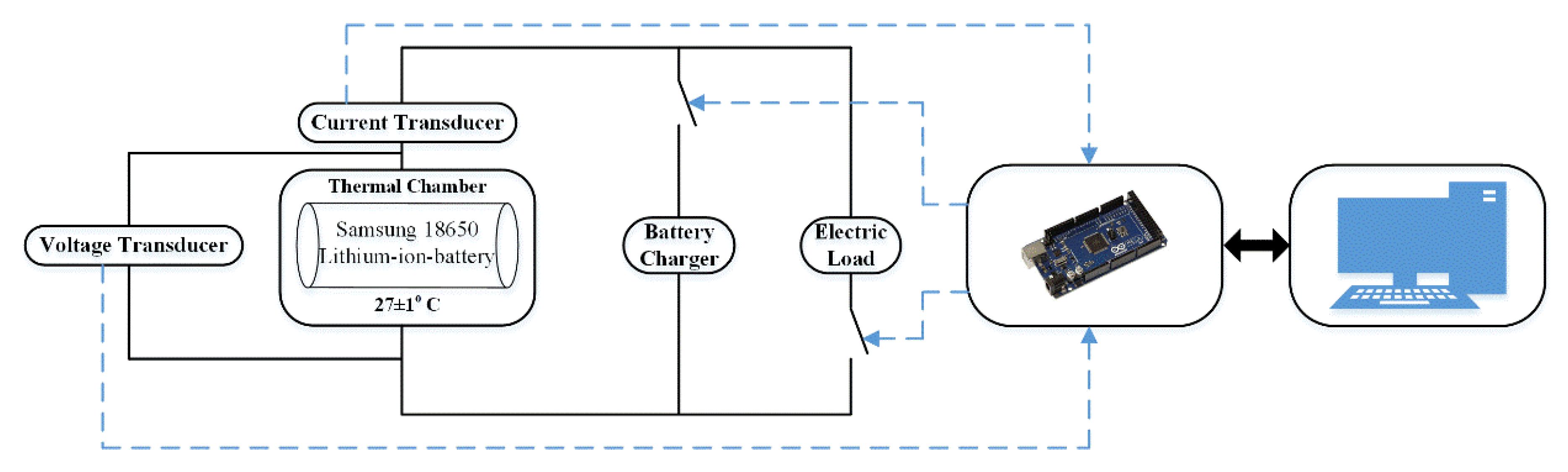
4. Experimental Setup and Estimated SOC

The experimental test configuration system is shown in Figure 4. The LIB was placed inside a thermal chamber to maintain the battery temperature at 27 ± 1 °C. The voltage and current transducer were used to measure and monitor terminal voltage and charge/discharge current at 1 s sample time. The transducers have a maximum measuring error of 0.25%. The Arduino mega 2560 interfaced with MATLAB^TM was used to control the charging and discharging of LIB.

The main specification of LIB used in this research work is listed in

Table 1. Specification of the tested LIB (Samsung ICR18650-26F) [36].

Type	Nominal Capacity	Maximum Discharge Current	Maximum Charge Current	Nominal Voltage	Discharge Cut-Off Voltage	Charge Termination Voltage
LICoO2	2600 mAh	2 C, 5.2 A	2.6 A	3.7 V	2.75 V	4.2 V

.

The OCV test for Samsung ICR18650-26F LIB cell was performed as mentioned in [37]. The average OCV of the charge and discharge cycle is retained to tackle the hysteresis phenomenon. The SOC-OCV function is highly nonlinear, which can be expressed in polynomial form as written below:

$$V_{ocv}=f\left(SOC\right)=a_{1}SO{C}^7+a_{2}SO{C}^6+a_{3}SO{C}^5+a_{4}SO{C}^4+a_{5}SO{C}^3+a_{6}SO{C}^2+a_{7}SOC+a_8$$

(36)

where $a$ is the values of the polynomial coefficient, which are listed in

Table 2. Values of $a$ for SOC-OCV function expressed in Equation (36).

Polynomial Coefficients	Values
a1	4.602 × 10−13
a2	−1.576 × 10−10
a3	2.103 × 10−8
a4	−1.386 × 10−6
a5	4.881 × 10−5
a6	1.056 × 10−3
a7	23.27× 10−3
a8	3.214

, and Figure 5 shows the OCV test result.

The estimated SOC results of both models are summed up in

Table 3. Comparison of first order and second order ARX battery models without uncertainties.

	First Order ARX Model	Second Order ARX Model
Computational speed (s)	1.1878	1.2831
Mean absolute error of SOC	0.94%	0.87%

. The slight supremacy of the second order ARX model is found on the first order ARX model with a slightly high computational complexity. These are well in-line with the literature [26,29]. To determine the computational speed of both models, the algorithm was run repeatedly for 10 times. The desktop-PC has the following specifications: 3.4 GHz CPU and 8.0 GB RAM.

5. Simulation Results

In this section, the impact of sensor accuracy/precision on battery modeled parameters and estimated SOC is evaluated for the following scenarios: (i) current sensor precision (ΔI) and (ii) voltage sensor precision (ΔV). The random error of the sensor accuracy simulated on MATLAB^TM and inserted in the measured value of voltage and current in Equations (9) and (20) to analyze their respective effects.

5.1. Sensitivity Analysis of First Order ARX Model

5.1.1. Current Sensor Accuracy/Precision Effect

In this work, the four values of ΔI (i.e., ±5 mA, ±50 mA, ±100 mA, and ±500 mA) are considered to analyze their respective effects on model identification, OCV, and SOC estimation. Figure 6a–c shows the identified model parameters, estimated OCV, and estimated SOC under different uncertainties in current sensor. It is evident from the Figures that the value of error in the parameters and estimated SOC increases with the increase in the sensor’s uncertainty. The maximum relative noted error in $R_{in}$, $R_{ap}$, and $C_{ap}$ are 0.06%, 3.74%, and 0.47% in the presence of 5 mA uncertainty, the current sensor accuracy mostly affected the value of $R_{in}$ and $R_{ap}$ as shown in Figure 6a. The noted root means square error (RMSE) in OCV estimation is 0.06 mV with 5 mA uncertainty in the measured current value, and the mean absolute error (MAE) in the SOC estimation is only 0.0091%. At 500 mA uncertainty in the measured current value, the maximum error in estimated SOC and OCV is 7.929% and 27.1 mV. The results of statistical error analysis are summed up in

Table 4. Statistical error analysis at different values of current sensors.

ΔI (mA)	Maximum Error		Root Means Square Error (RMSE)		Mean Absolute Error (MAE)
	$\mathit{S}\mathit{O}\mathit{C}{ }^1(\%)$	$\mathit{O}\mathit{C}\mathit{V}\left(\mathbf{mV}\right)$	$\mathit{S}\mathit{O}\mathit{C}{ }^1(\%)$	$\mathit{O}\mathit{C}\mathit{V}\left(\mathbf{mV}\right)$	$\mathit{S}\mathit{O}\mathit{C}{ }^1(\%)$	$\mathit{O}\mathit{C}\mathit{V}\left(\mathbf{mV}\right)$
5	0.0667	0.26	0.01	0.06	0.0091	0.05
50	0.8784	2.90	0.13	0.68	0.0962	0.54
100	1.6955	5.40	0.27	1.40	0.1945	1.10
500	7.929	27.1	1.36	6.90	0.9729	5.50

¹ It does not include modelling error. Modelling MAE of first order ARX = 0.94%.

.

5.1.2. Voltage Sensor Accuracy/Precision Effect

In this work, the four values of ΔV (i.e., ±1 mV, ±2.5 mV, ±5.0 mV, and ±10 mV) are considered to analyze their respective effects on model identification, OCV, and SOC estimation. Figure 7a–c shows the identified model parameters, estimated OCV, and estimated SOC under different uncertainties in voltage sensor. It is evident from the Figures that the value of error in the parameters and estimated SOC rapidly increases with the increase in the sensor’s uncertainty as compared to uncertainty in current sensor. The maximum relative noted error in $R_{in}$, $R_{ap}$, and $C_{ap}$ are 0.2%, 0.96%, and 2.41% in the presence of 5 mV uncertainty. The noted RMSE in OCV estimation is 1.4 mV with 5 mV uncertainty in the measured value and the MAE in the SOC estimation is only 0.20%. At 10 mV uncertainty in the measured value, the maximum error in estimated SOC and OCV is 3.30% and 1.1 mV. The results of statistical error analysis are summed up in

Table 5. Statistical error analysis at different values of voltage sensors.

ΔV (mV)	Maximum Error		Root Means Square Error (RMSE)		Mean Absolute Error (MAE)
	$\mathit{S}\mathit{O}\mathit{C}{ }^1(\%)$	$\mathit{O}\mathit{C}\mathit{V}\left(\mathbf{mV}\right)$	$\mathit{S}\mathit{O}\mathit{C}{ }^1(\%)$	$\mathit{O}\mathit{C}\mathit{V}\left(\mathbf{mV}\right)$	$\mathit{S}\mathit{O}\mathit{C}{ }^1(\%)$	$\mathit{O}\mathit{C}\mathit{V}\left(\mathbf{mV}\right)$
1	0.33	1.0	0.05	0.2	0.03	0.2
2.5	0.78	2.6	0.12	0.6	0.08	0.4
5	1.69	5.2	0.28	1.4	0.20	1.1
10	3.30	1.1	0.53	2.7	0.37	2.2

¹ It does not include modelling error. Modelling MAE of first order ARX = 0.94%.

.

5.2. Sensitivity Analysis of Second Order ARX Model

5.2.1. Current Sensor Accuracy/Precision Effect

In sensitivity analysis of second order ARX model same values of ΔI (i.e., ±5 mA, ±50 mA, ±100 mA, and ±500 mA) are considered to analyze their respective effects on model identification, OCV, and SOC estimation. The same current error value was used to identify and estimate the states of both (first and second order ARX) models. Figure 8a–c shows the identified model parameters, estimated OCV, and estimated SOC under different uncertainties in current sensor. It is evident from the Figures that the value of error in the parameters and estimated SOC increases with the increase in the sensor’s uncertainty. The maximum relative noted error in $R_{in}$, $R_{ap}$, $C_{ap}$, $R_{cp}$, and $C_{cp}$ are 6.6%, 40%, 1.8%, 33%, and 2.2% in the presence of 500 mA uncertainty, the current sensor accuracy mostly affected the value of $R_{in}$, $R_{ap}$, and $R_{cp}$ as shown in Figure 8a. The noted RMSE in OCV estimation is 1.25 mV with 500 mA uncertainty in the measured current value and the MAE in the SOC estimation is only 0.9501%. The results of statistical error analysis are summed up in

Table 6. Statistical error analysis at different values of current sensors.

ΔI. (mA)	Maximum Error		Root Means Square Error (RMSE)		Mean Absolute Error (MAE)
	$\mathit{S}\mathit{O}\mathit{C}{ }^1(\%)$	$\mathit{O}\mathit{C}\mathit{V}\left(\mathbf{mV}\right)$	$\mathit{S}\mathit{O}\mathit{C}{ }^1(\%)$	$\mathit{O}\mathit{C}\mathit{V}\left(\mathbf{mV}\right)$	$\mathit{S}\mathit{O}\mathit{C}{ }^1(\%)$	$\mathit{O}\mathit{C}\mathit{V}\left(\mathbf{mV}\right)$
5	0.0691	0.24	0.01	0.05	0.0084	0.04
50	0.7021	2.01	0.11	0.58	0.0725	0.47
100	1.2134	5.02	0.31	1.44	0.2112	1.12
500	2.7016	34.7	1.25	6.43	0.9501	5.32

¹ It does not include modelling error. Modelling MAE of second order ARX = 0.87%.

.

5.2.2. Voltage Sensor Accuracy/Precision Effect

In sensitivity analysis of second order ARX model same values of ΔV (i.e., ±1 mV, ±2.5 mV, ±5.0 mV, and ±10 mV) are considered to analyze their respective effects on model identification, OCV, and SOC estimation. The same voltage sensor error value was used to identify and estimate the states of both (first and second order ARX) models. Figure 9a–c shows the identified model parameters, estimated OCV, and estimated SOC under different uncertainties in current sensor. It is clear from the Figures that the value of error in the parameters and estimated SOC increases with the increase in the sensor’s uncertainty. The relative error profile of $R_{in}$, $R_{ap}$, $C_{ap}$, $R_{cp}$, and $C_{cp}$ is shown in Figure 9a. The results of statistical error analysis of voltage sensor are listed in

Table 7. Statistical error analysis at different values of voltage sensors.

ΔV (mV)	Maximum Error		Root Means Square Error (RMSE)		Mean Absolute Error (MAE)
	$\mathit{S}\mathit{O}\mathit{C}{ }^1(\%)$	$\mathit{O}\mathit{C}\mathit{V}\left(\mathbf{mV}\right)$	$\mathit{S}\mathit{O}\mathit{C}{ }^1(\%)$	$\mathit{O}\mathit{C}\mathit{V}\left(\mathbf{mV}\right)$	$\mathit{S}\mathit{O}\mathit{C}{ }^1(\%)$	$\mathit{O}\mathit{C}\mathit{V}\left(\mathbf{mV}\right)$
1	0.0941	1.03	0.03	0.25	0.0226	0.19
2.5	0.7234	0.67	0.06	0.41	0.0532	0.34
5	1.1959	1.64	0.19	1.12	0.1799	1.01
10	2.7246	3.03	0.34	2.21	0.3250	2.00

¹ It does not include modelling error. Modelling MAE of second order ARX = 0.87%.

.

6. Discussion

Some evocative results can be drawn using the simulated results presented in Section 5.

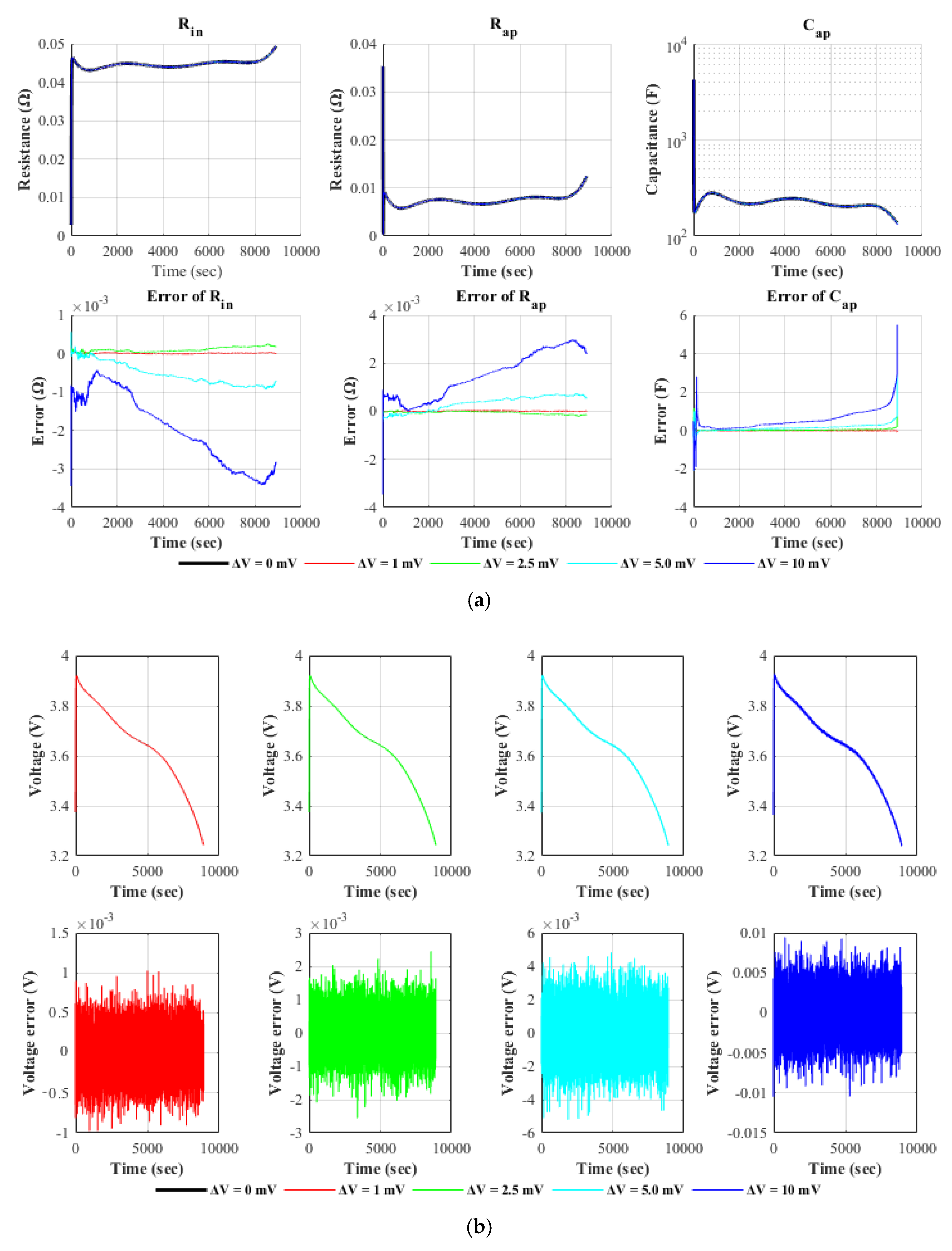
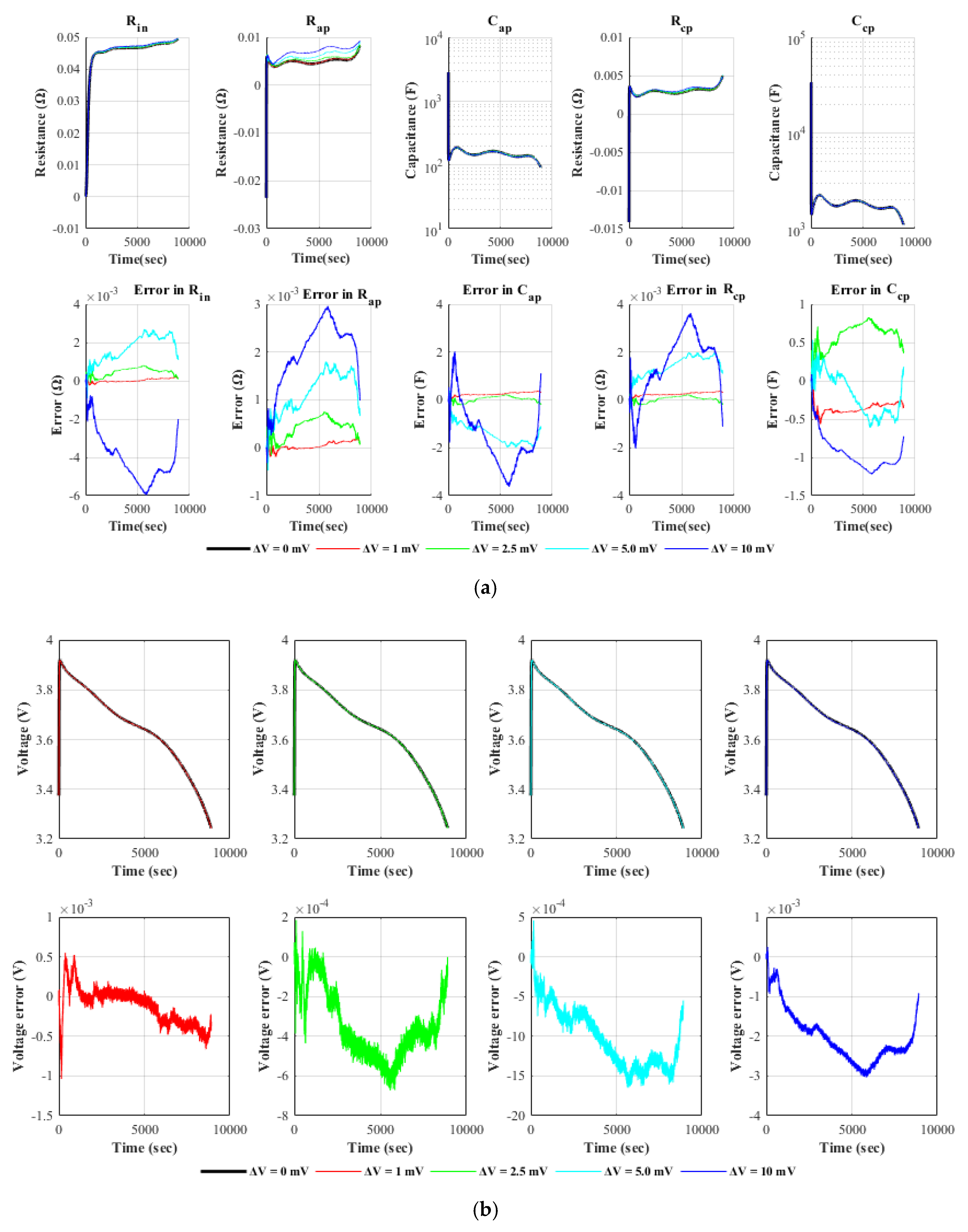
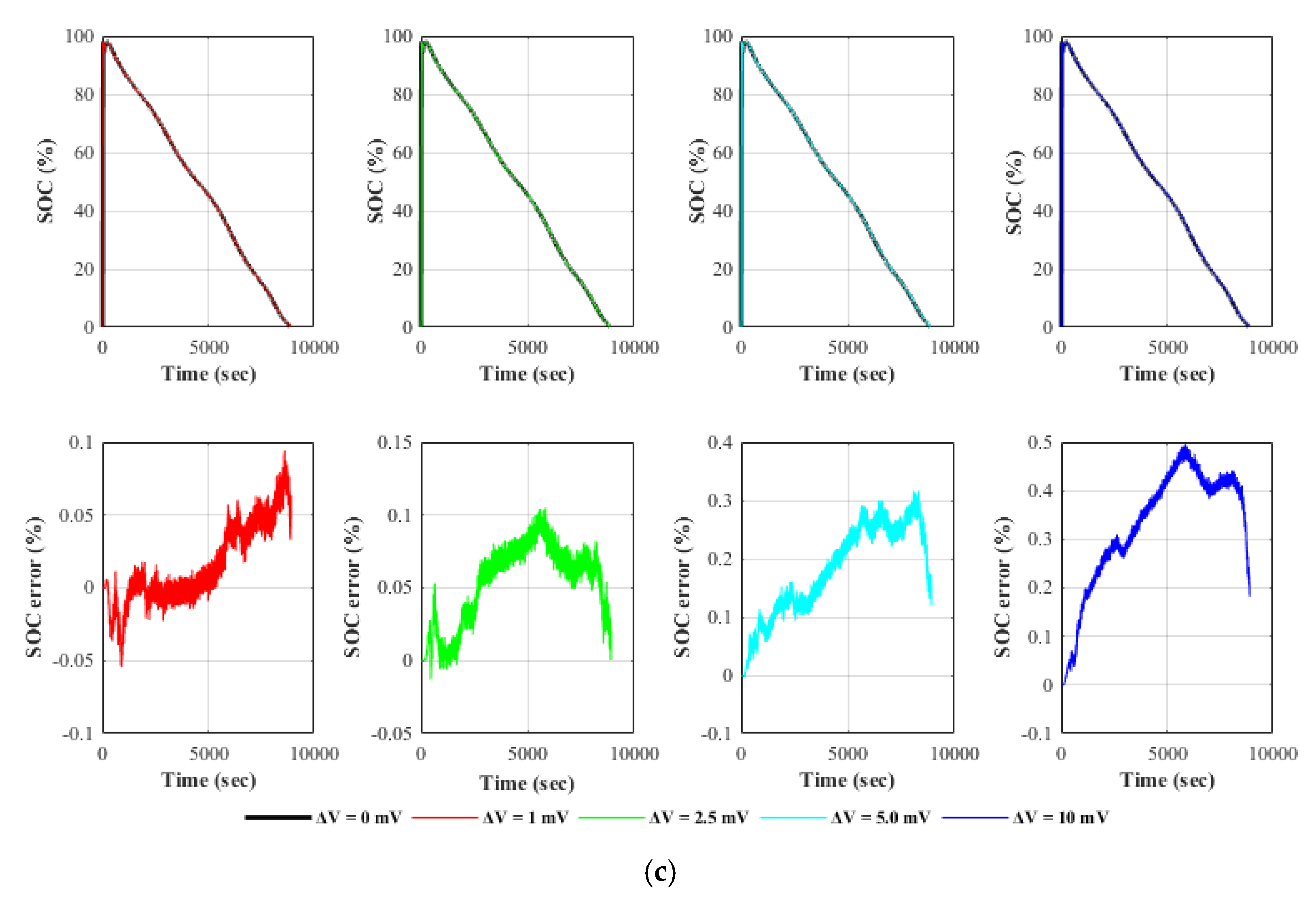
Different variations of voltage transducer precision (i.e., ±1 mV, ±2.5 mV, ±5 mV, and ±10 mV) were applied for parameter identification and SOC estimation of both (1RC and 2RC) ARX models. The results reveal that the small variation in voltage sensor accuracy has a significant impact on model accuracy and model accuracy has a direct effect on SOC estimation. When the uncertainty of ±1 mV was applied to the measured voltage values, an increase of 0.03% and 0.02% in the MAE was noted for first and second order ARX models, respectively. In case of ±10 mV uncertainty, the change in maximum noted the errors of SOC estimation are 3.30% and 2.72% for first and second order RC models respectively, which is not acceptable for SOC estimation of LIB. It is also important to note that the small change in ΔV has a huge influence on model parameters and SOC estimation as shown in Table 5 and Table 7. Therefore, to ensure the accurate estimation of model parameters and SOC, it is recommended that the accuracy of the voltage sensor must be high, and it should be less than ±2.5 mV.

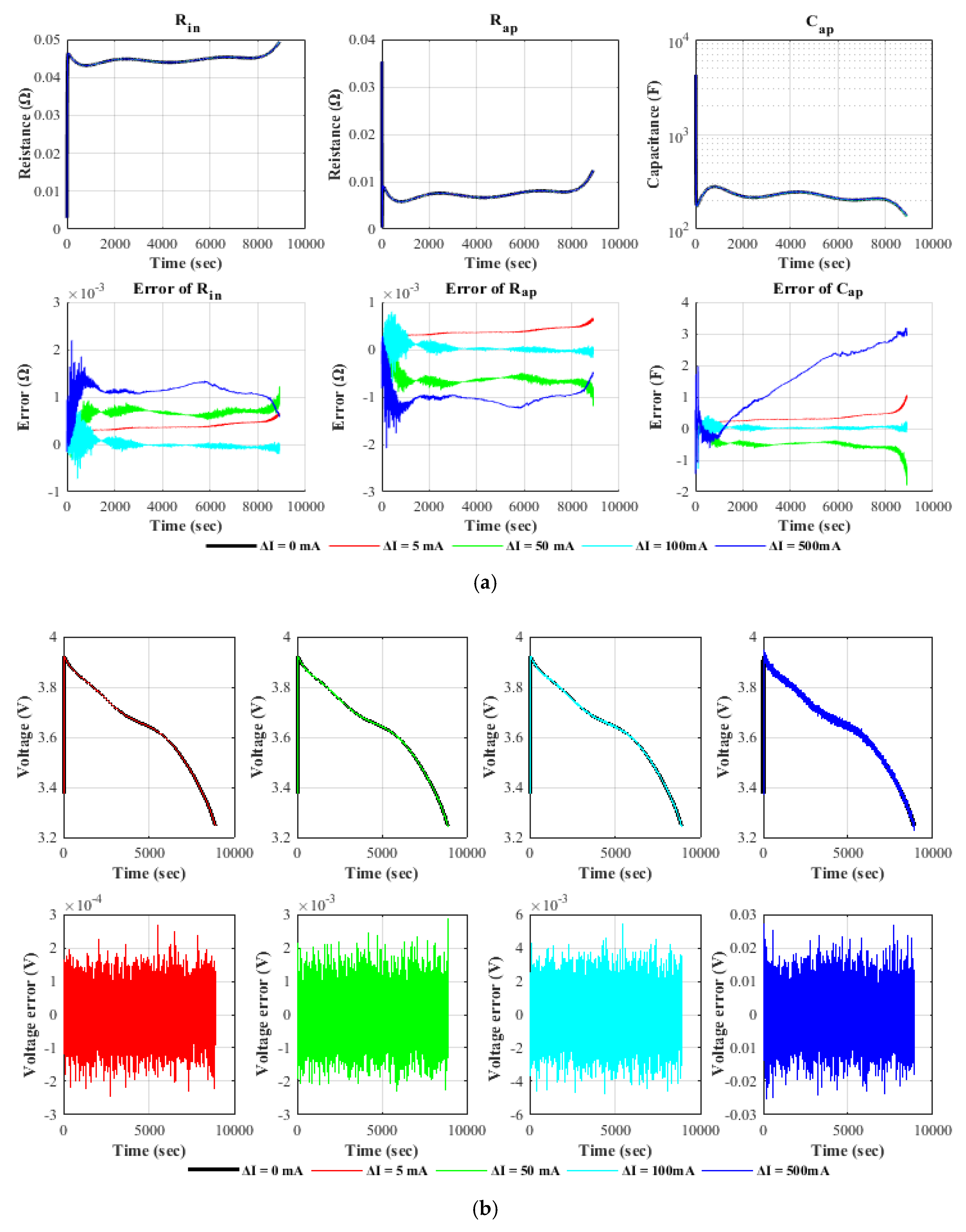
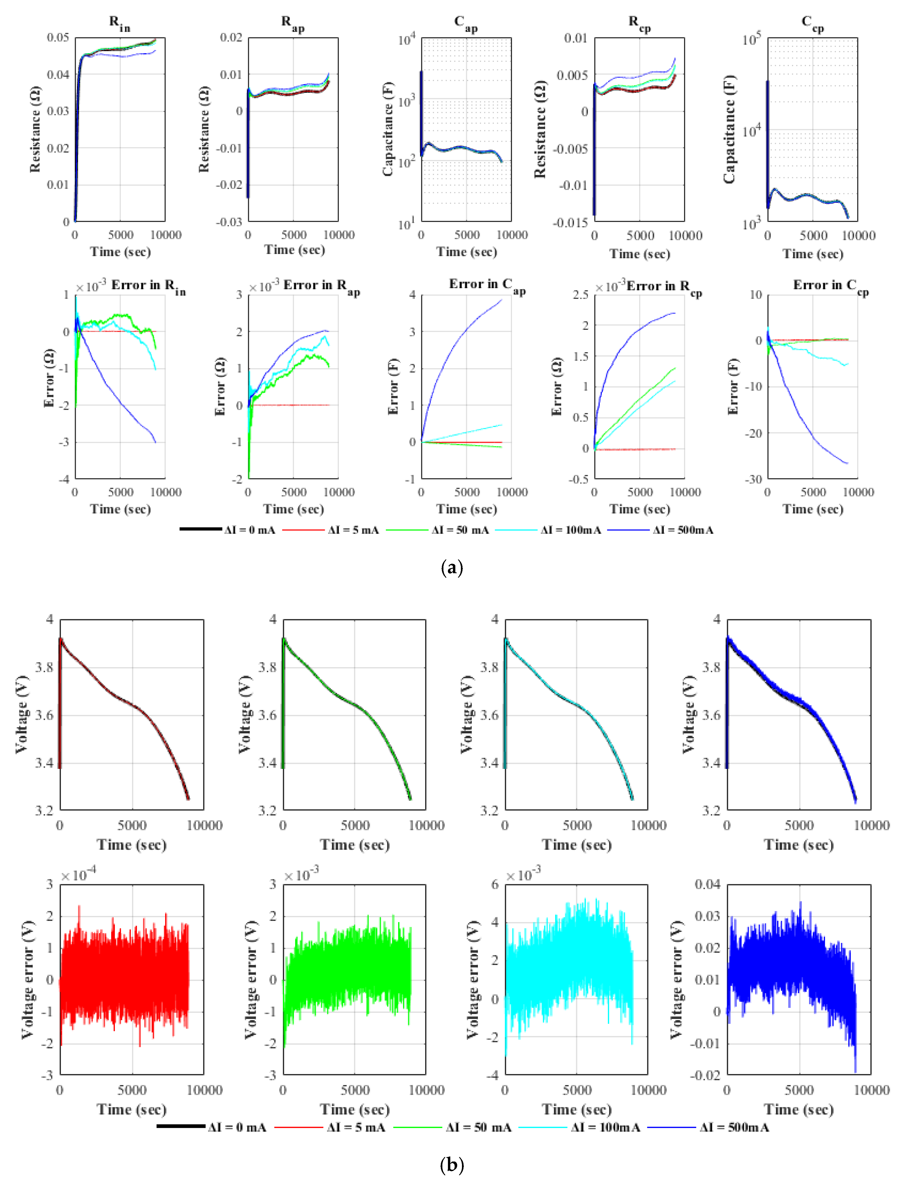
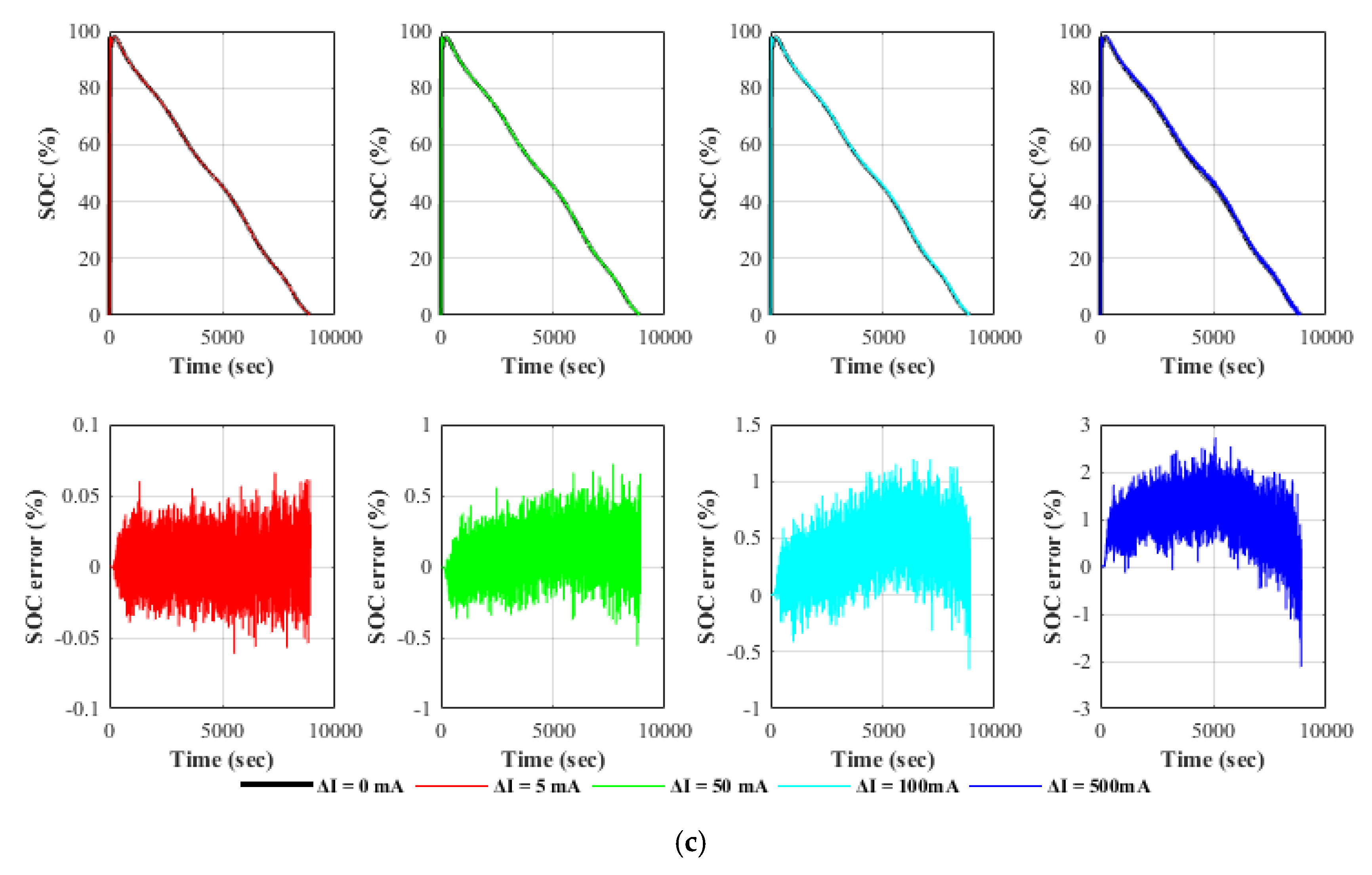
Similarly, different uncertainties (i.e., ±5 mA, ±50 mA, ±100 mA, and ±500 mA) in current sensor accuracy were also applied for model identification and SOC estimation of both (1RC and 2RC) ARX models. The current transducer sensitivity has an adverse influence on the model’s parameter and SOC estimation. The error of ±5 mA and ±50 mA in the measured battery’s current has a negligible influence on the accuracy of estimated SOC. As the value of error increased to ±0.1 A in 1RC battery model, the changes in the maximum SOC error and MAE are 1.69% and 0.19% respectively (Table 4). The changes in MAE and maximum error for the 2RC model at ±0.5 A are 0.95% and 2.70% respectively (Table 6). It is important to note that the small inaccuracy in the measured current did not have any drastic effect on the accuracy of estimated SOC as compared to voltage sensor inaccuracy. Therefore, to confine the SOC and parameters accuracy, the current accuracy should be less than ±0.05 A.

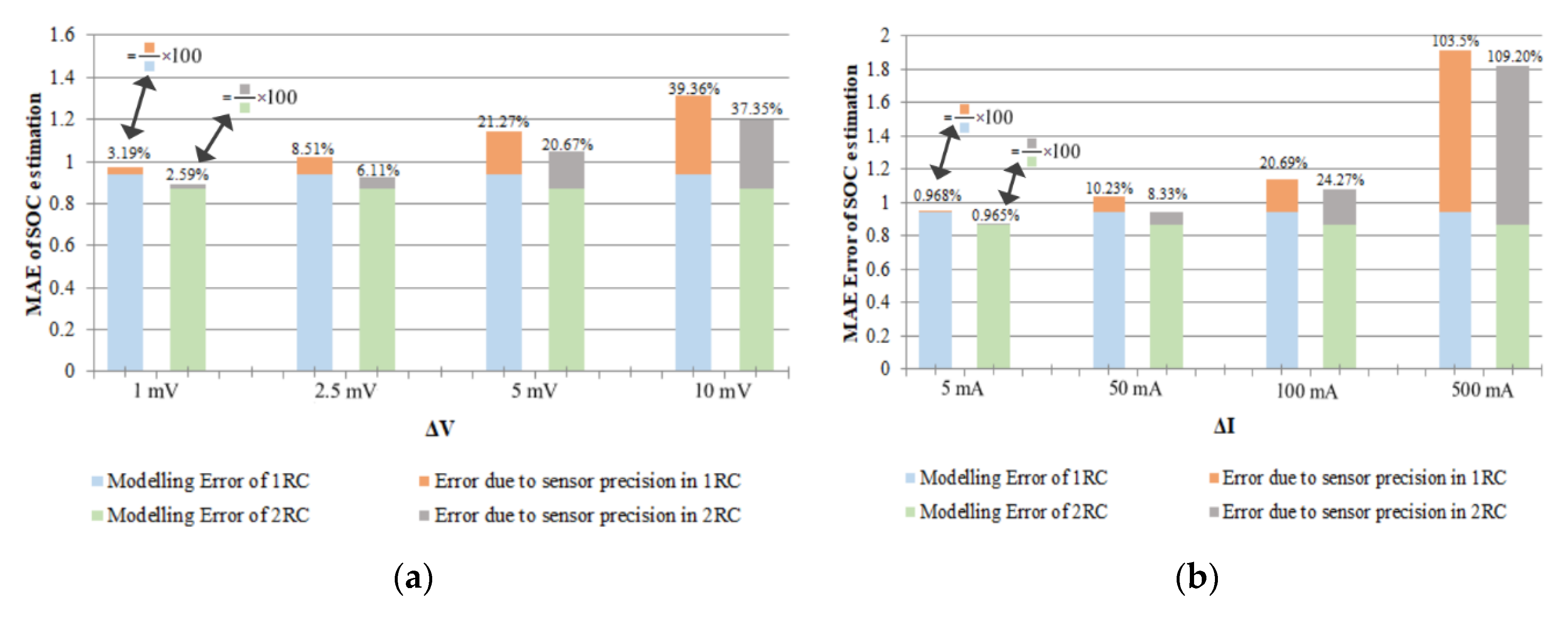
The second order RC battery model has better accuracy and high complexity compared to the 1RC battery model. The listed error values in Table 4, Table 5, Table 6 and Table 7 show only the error due to the sensor’s sensitivity. The MAE and relative MAE of both models are compared in Figure 10. From the results presented in Table 4, Table 5, Table 6 and Table 7 and Figure 10, the sensor errors have the same influence on the SOC estimation of both models. Therefore, it can be concluded that the error in sensor sensitivity has no direct association with the structure and complexity of the battery model.

7. Conclusions

In this work, the impact of sensor sensitivity was analyzed to observe their respective influences on parameter identification and SOC estimation. First and second order ARX battery models were adopted to evaluate the impact of sensor sensitivity. The battery was modeled using the Lagrange multiplier method. The voltage sensor error (i.e., ±1 mV, ±2.5 mV, ±5 mV, and ±10 mV) and current sensor error (i.e., ±5 mA, ±50 mA, ±100 mA, and ±500 mA) were simulated and inserted in the measured values. The results reveal that the voltage sensitivity has a very high impact on SOC estimation, and the accuracy of the voltage sensor should be ≥0.05% (with 5 V range) for first order MAE ≤1.02% and second order MAE ≤0.92%. The current sensory uncertainty has a lesser impact as compared to the voltage sensor. The accuracy of the current sensor ≥0.5% (with 10 A range) for first order MAE ≤1.03% and second order MAE ≤0.94%. The comparative analysis of both models revealed that the uncertainties in both sensors have the same influence on the SOC estimation despite the type of battery models.

References

1. Eberle, U.; Von Helmolt, R. Sustainable transportation based on electric vehicle concepts: A brief overview. Energy Environ. Sci. 2010, 3, 689–699. [Google Scholar] [CrossRef]
2. Tanaka, N. Technology Roadmap: Electric and Plug-In Hybrid. Electric Vehicles; Technical Report; International Energy Agency: Paris, France, 2011; Available online: https://www.iea.org/publications/freepublications/.../EV_PHEV_Roadmap.pdf (accessed on 21 June 2019).
3. Contestabile, M.; Offer, G.; Slade, R.; Jaeger, F.; Thoennes, M. Battery electric vehicles, hydrogen fuel cells and biofuels. Which will be the winner? Energy Environ. Sci. 2011, 4, 3754–3772. [Google Scholar] [CrossRef]
4. Hussain, S.; Ali, M.U.; Nengroo, S.H.; Khan, I.; Ishfaq, M.; Kim, H.-J. Semiactive Hybrid Energy Management System: A Solution for Electric Wheelchairs. Electronics 2019, 8, 345. [Google Scholar] [CrossRef]
5. Ralon, P.; Taylor, M.; Ilas, A.; Diaz-Bone, H.; Kairies, K. Electricity Storage and Renewables: Costs and Markets to 2030; International Renewable Energy Agency: Abu Dhabi, UAE, 2017; Available online: https://www.irena.org/-/media/Files/.../IRENA_Electricity_Storage_Costs_2017.pdf (accessed on 21 June 2019).
6. Umair Ali, M.; Hussain Nengroo, S.; Adil Khan, M.; Zeb, K.; Ahmad Kamran, M.; Kim, H.-J. A real-time simulink interfaced fast-charging methodology of lithium-ion batteries under temperature feedback with fuzzy logic control. Energies 2018, 11, 1122. [Google Scholar] [CrossRef]
7. Khan, M.A.; Zeb, K.; Sathishkumar, P.; Ali, M.U.; Uddin, W.; Hussain, S.; Ishfaq, M.; Khan, I.; Cho, H.-G.; Kim, H.-J. A Novel Supercapacitor/Lithium-Ion Hybrid Energy System with a Fuzzy Logic-Controlled Fast Charging and Intelligent Energy Management System. Electronics 2018, 7, 63. [Google Scholar] [CrossRef]
8. Hussain Nengroo, S.; Umair Ali, M.; Zafar, A.; Hussain, S.; Murtaza, T.; Junaid Alvi, M.; Raghavendra, K.V.G.; Jee Kim, H. An Optimized Methodology for a Hybrid Photo-Voltaic and Energy Storage System Connected to a Low-Voltage Grid. Electronics 2019, 8, 176. [Google Scholar] [CrossRef]
9. Nengroo, S.; Kamran, M.; Ali, M.; Kim, D.-H.; Kim, M.-S.; Hussain, A.; Kim, H. Dual battery storage system: An optimized strategy for the utilization of renewable photovoltaic energy in the United Kingdom. Electronics 2018, 7, 177. [Google Scholar] [CrossRef]
10. Ali, M.U.; Zafar, A.; Nengroo, S.H.; Hussain, S.; Junaid Alvi, M.; Kim, H.-J. Towards a Smarter Battery Management System for Electric Vehicle Applications: A Critical Review of Lithium-Ion Battery State of Charge Estimation. Energies 2019, 12, 446. [Google Scholar] [CrossRef]
11. Hannan, M.A.; Lipu, M.H.; Hussain, A.; Mohamed, A. A review of lithium-ion battery state of charge estimation and management system in electric vehicle applications: Challenges and recommendations. Renew. Sustain. Energy Rev. 2017, 78, 834–854. [Google Scholar] [CrossRef]
12. He, H.; Xiong, R.; Zhang, X.; Sun, F.; Fan, J. State-of-Charge Estimation of the Lithium-Ion Battery Using an Adaptive Extended Kalman Filter Based on an Improved Thevenin Model. IEEE Trans. Veh. Technol. 2011, 60, 1461–1469. [Google Scholar] [CrossRef]
13. Ali, M.; Kamran, M.; Kumar, P.; Nengroo, S.; Khan, M.; Hussain, A.; Kim, H.-J. An Online Data-Driven Model Identification and Adaptive State of Charge Estimation Approach for Lithium-ion-Batteries Using the Lagrange Multiplier Method. Energies 2018, 11, 2940. [Google Scholar] [CrossRef]
14. He, Z.; Gao, M.; Wang, C.; Wang, L.; Liu, Y. Adaptive State of Charge Estimation for Li-Ion Batteries Based on an Unscented Kalman Filter with an Enhanced Battery Model. Energies 2013, 6, 4134–4151. [Google Scholar] [CrossRef] [Green Version]
15. Xing, Y.; He, W.; Pecht, M.; Tsui, K.L. State of charge estimation of lithium-ion batteries using the open-circuit voltage at various ambient temperatures. Appl. Energy 2014, 113, 106–115. [Google Scholar] [CrossRef]
16. Yang, S.; Deng, C.; Zhang, Y.; He, Y. State of Charge Estimation for Lithium-Ion Battery with a Temperature-Compensated Model. Energies 2017, 10, 1560. [Google Scholar] [CrossRef]
17. Wang, Y.; Zhang, C.; Chen, Z. A method for joint estimation of state-of-charge and available energy of LiFePO4 batteries. Appl. Energy 2014, 135, 81–87. [Google Scholar] [CrossRef]
18. Tian, Y.; Xia, B.; Sun, W.; Xu, Z.; Zheng, W. A modified model based state of charge estimation of power lithium-ion batteries using unscented Kalman filter. J. Power Sources 2014, 270, 619–626. [Google Scholar] [CrossRef]
19. Zheng, L.; Zhang, L.; Zhu, J.; Wang, G.; Jiang, J. Co-estimation of state-of-charge, capacity and resistance for lithium-ion batteries based on a high-fidelity electrochemical model. Appl. Energy 2016, 180, 424–434. [Google Scholar] [CrossRef]
20. Chaoui, H.; Ibe-Ekeocha, C.C.; Gualous, H. Aging prediction and state of charge estimation of a LiFePO4 battery using input time-delayed neural networks. Electr. Power Syst. Res. 2017, 146, 189–197. [Google Scholar] [CrossRef]
21. Xiong, R.; Sun, F.; Chen, Z.; He, H. A data-driven multi-scale extended Kalman filtering based parameter and state estimation approach of lithium-ion olymer battery in electric vehicles. Appl. Energy 2014, 113, 463–476. [Google Scholar] [CrossRef]
22. Zheng, Y.; Ouyang, M.; Han, X.; Lu, L.; Li, J. Investigating the error sources of the online state of charge estimation methods for lithium-ion batteries in electric vehicles. J. Power Sources 2018, 377, 161–188. [Google Scholar] [CrossRef]
23. Liu, X.; Chen, Z.; Zhang, C.; Wu, J. A novel temperature-compensated model for power Li-ion batteries with dual-particle-filter state of charge estimation. Appl. Energy 2014, 123, 263–272. [Google Scholar] [CrossRef]
24. Xia, B.; Chen, C.; Tian, Y.; Sun, W.; Xu, Z.; Zheng, W. A novel method for state of charge estimation of lithium-ion batteries using a nonlinear observer. J. Power Sources 2014, 270, 359–366. [Google Scholar] [CrossRef]
25. Zhang, X.; Mi, C. Vehicle Power Management: Modeling, Control and Optimization; Springer Science & Business Media: London, UK, 2011. [Google Scholar]
26. Lai, X.; Zheng, Y.; Sun, T. A comparative study of different equivalent circuit models for estimating state-of-charge of lithium-ion batteries. Electrochim. Acta 2018, 259, 566–577. [Google Scholar] [CrossRef]
27. Yuan, S.; Wu, H.; Ma, X.; Yin, C. Stability analysis for li-ion battery model parameters and state of charge estimation by measurement uncertainty consideration. Energies 2015, 8, 7729–7751. [Google Scholar] [CrossRef]
28. Hu, X.; Li, S.; Peng, H. A comparative study of equivalent circuit models for Li-ion batteries. J. Power Sources 2012, 198, 359–367. [Google Scholar] [CrossRef]
29. Zhang, L.; Peng, H.; Ning, Z.; Mu, Z.; Sun, C. Comparative research on RC equivalent circuit models for lithium-ion batteries of electric vehicles. Appl. Sci. 2017, 7, 1002. [Google Scholar] [CrossRef]
30. Xia, B.; Wang, H.; Tian, Y.; Wang, M.; Sun, W.; Xu, Z. State of charge estimation of lithium-ion batteries using an adaptive cubature Kalman filter. Energies 2015, 8, 5916–5936. [Google Scholar] [CrossRef]
31. Wei, Z.; Zhao, J.; Ji, D.; Tseng, K.J. A multi-timescale estimator for battery state of charge and capacity dual estimation based on an online identified model. Appl. Energy 2017, 204, 1264–1274. [Google Scholar] [CrossRef]
32. Rahimi-Eichi, H.; Ojha, U.; Baronti, F.; Chow, M.-Y. Battery management system: An overview of its application in the smart grid and electric vehicles. IEEE Ind. Electron. Mag. 2013, 7, 4–16. [Google Scholar] [CrossRef]
33. Hu, X.; Jiang, J.; Cao, D.; Egardt, B. Battery health prognosis for electric vehicles using sample entropy and sparse Bayesian predictive modeling. IEEE Trans. Ind. Electron. 2015, 63, 2645–2656. [Google Scholar] [CrossRef]
34. Dyer, C.K.; Moseley, P.T.; Ogumi, Z.; Rand, D.A.; Scrosati, B. Encyclopedia of Electrochemical Power Sources; Elsevier Science & Technology: Amsterdam, The Netherlands, 2009. [Google Scholar]
35. Wenzl, H. BATTERIES AND FUEL CELLS | Efficiency. In Encyclopedia of Electrochemical Power Sources; Garche, J., Ed.; Elsevier: Amsterdam, The Netherlands, 2009; pp. 544–551. [Google Scholar]
36. Samsung, S. Specification of Product for Lithium-Ion Rechargeable Cell Model: Icr18650-26f. 2009. Available online: https://ultrafire.es/files/ICR18650-26F.pdf (accessed on 21 June 2019).
37. Abu-Sharkh, S.; Doerffel, D. Rapid test and non-linear model characterisation of solid-state lithium-ion batteries. J. Power Sources 2004, 130, 266–274. [Google Scholar] [CrossRef]
Figure 1. Schematic diagram of first order RC ARX battery model for lithium-ion battery.
Electronics 08 00709 g001
Figure 2. Schematic diagram of second order RC ARX battery model for lithium-ion battery.
Electronics 08 00709 g002
Figure 3. Flow diagram for OCV and SOC estimation.
Electronics 08 00709 g003
Figure 4. Experimental setup.
Electronics 08 00709 g004
Figure 5. SOC-OCV curve of LIB.
Electronics 08 00709 g005
Figure 6. Estimated values at different precision of current sensors: (a) model parameters; (b) estimated OCV; (c) estimated SOC.
Electronics 08 00709 g006aElectronics 08 00709 g006b
Figure 7. Estimated values at different precision of voltage sensors: (a) model parameters; (b) estimated OCV; (c) estimated SOC.
Electronics 08 00709 g007aElectronics 08 00709 g007b
Figure 8. Estimated values at different precision of current sensors: (a) model parameters; (b) estimated OCV; (c) estimated SOC.
Electronics 08 00709 g008aElectronics 08 00709 g008b
Figure 9. Estimated values at different precision of voltage sensors: (a) model parameters; (b) estimated OCV; (c) estimated SOC.
Electronics 08 00709 g009aElectronics 08 00709 g009b
Figure 10. Comparison of first and second order ARX battery models; (a) At different uncertainties in measured voltage value; (b) At different uncertainties in measured current value.
Electronics 08 00709 g010