Article

Scenario-Based Emergency Material Scheduling Using V2X Communications

1
School of Automobile, Chang’an University, Xi’an 710064, China
2
Traffic and Plan Design Institute, Huzhou 313000, China
3
Department of Information Technology and Electrical Engineering, University of Oulu, 90014 Oulu, Finland
4
Department of Electrical and Computer Engineering, University of Toronto, Toronto, ON M5S 3G4, Canada
*
Authors to whom correspondence should be addressed.
Electronics 2019, 8(6), 707; https://doi.org/10.3390/electronics8060707
Submission received: 11 May 2019 / Revised: 19 June 2019 / Accepted: 19 June 2019 / Published: 22 June 2019
(This article belongs to the Special Issue Smart, Connected and Efficient Transportation Systems)

Abstract

:
Vehicle-to-everything (V2X) communications can be applied in emergency material scheduling due to their performance in collecting and transmitting disaster-related data in real time. The urgency of disaster depots can be judged based on the disaster area video, and the scenario coefficient can be evaluated for building a fairness model. This paper presents a scenario-based approach for emergency material scheduling (SEMS) using V2X communications. We propose a SEMS model, with the objectives of minimum time and maximum fairness in the cases of multiple supply depots, disaster depots, commodities and transport modes for logistics management of relief commodities. We design the SEMS algorithm based on the artificial fish-swarm algorithm to obtain an optimized solution. The results demonstrate that the SEMS model can enhance the fairness of relief scheduling, especially for disaster depots with small demands compared to the Gini and enhanced Theil fairness models. Moreover, the acquired vehicle speed via V2X communications updates the SEMS model in real time, which approaches a solution closer to reality.

1. Introduction

Emergency logistics is receiving increasing attention from academics as well as practitioners [1,2,3]. Effective and efficient delivery of relief resources to victims is critical. However, unreasonable distribution of emergency material seriously affects the efficiency of disaster rescue. Emergency material scheduling refers to a quick response to the urgent need for relief in affected areas right after disasters, especially emergency logistics distribution. Traditional emergency material scheduling has many shortcomings, for example, the simplification of dynamic information on traffic such as speed, road traffic capacity, road network repairing, lack of fairness, and ignorance of differences of disaster scenarios, including air transportation, making it hard to implement an optimal scheduling plan, especially when the supply is insufficient. In recent years, vehicle-to-everything (V2X) communication has provided a useful tool for making more precise relief logistics decisions by collecting and transmitting disaster video and vehicle data in real time.
Vehicle-to-everything communication incorporates communications such as V2I (vehicle-to-infrastructure), V2N (vehicle-to-network), V2V (vehicle-to-vehicle), V2P (vehicle-to-pedestrian), V2D (vehicle-to-device) and V2G (vehicle-to-grid). The main motivations for V2X are road safety, traffic efficiency and energy savings [4]. V2I and V2V communication can be used to share relevant information, such as vehicle position, damage to the roads, and surrounding environment, especially in an earthquake [5,6]. A vehicle-mounted communication system can collect the vehicle running status by using Controller Area Network (CAN) bus and sensors, such as vehicle location, running direction, running speed, acceleration, and surrounding video. With V2X communications, the urgency of a disaster scenario can be evaluated accurately and considered in the optimization of emergency material scheduling, which is a novelty of our method.
This paper studies a scenario-based emergency material scheduling method (SEMS), taking into account the urgency of a disaster scenario and the fairness of material scheduling. The SEMS takes fairness as the main objective and the transport time as the secondary objective, and fairness also considers the urgency of a disaster scenario besides traditional demand satisfaction of material scheduling.
The remainder of the paper is organized as follows. Section 2 reviews related works. Section 3 presents the SEMS method. Section 4 presents the experiment to verify the SEMS model. Section 5 presents conclusions and future work.

2. Literature Review

Various programming models have been developed for emergency logistics, including linear programming, integer or mixed integer programming, and mixed integer linear programming [7,8]. Safeer et al. [9] employed a classification-based method to identify cost functions and constraints for primary emergency operations in relief distribution. Hamedi et al. [10] addressed the reliable humanitarian response planning for a fleet of vehicles and proposed a genetic algorithm. Ferrer et al. [11] built a compromise programming model for multi-criteria optimization in last-mile humanitarian distribution. The model is able to produce an actual vehicle schedule while forcing vehicles to form convoys in humanitarian operation research. Ahmadi et al. [12] proposed a multi-warehouse location-route model considering network failures, multiple vehicle use and standard rescue time, which could significantly reduce scheduling time at the expense of more local warehouses and vehicles. Owusu-Kwateng et al. [13] evaluated the performance of relief logistics in a disaster in Ghana with emphasis on the coordination of emergency relief operation and effectiveness of inventory management. Rahafrooz et al. [14] proposed a multi-objective robust possibilistic programming model, which simultaneously considered maximizing the distributive justice in emergency material scheduling, minimizing the risk of relief distribution, and minimizing the total logistics costs.
Many researchers took into account uncertainty in relief distribution and developed stochastic programming models or robust optimization models [15,16]. Najafi et al. [17] proposed a multi-objective stochastic model to manage the logistics in earthquakes. Ransikarbum et al. [18] used the triangular fuzzy number to describe the emergency demands and introduced the time-dependent function to simulate the dynamic road network. Liu et al. [19] presented a Petri net-based method E-Net for an emergency response process constrained by resources and uncertain duration. Bozorgiamiri et al. [20] developed a multi-objective robust stochastic programming approach for the emergency material scheduling under uncertainty. Not only demands but also supplies and the cost of procurement and transportation were considered as the uncertain parameters.
For emergency material scheduling, it is an important indicator to improve the overall demand satisfaction of the disaster areas and guarantee the fairness simultaneously. In recent years, fairness has been widely studied. According to [21], the Theil L index is sensitive to low income. Emergency material scheduling (EMS) cannot ignore the disaster areas with low demands, so we chose the Theil L index to indicate the fairness of material scheduling. Chen et al. [22] took the satisfaction of the whole disaster areas as the objective and built a model for multi-commodity, multi-supply depot, multi-disaster depot, and multi-mode of transportation, so as to maximize the rescue efficiency of EMS. Mishra et al. [23] applied two basic round-robin-based greedy search algorithms and proposed an optimized algorithm for fair delivery of relief supplies. Chang et al. [24] dynamically adjusted the distribution schedules from various supply depots according to the requirements at demand depots to minimize unsatisfied demand for resources, time for delivery, and transportation costs. However, they researched fairness from the perspective of demand satisfaction and ignored the impacts of different disaster scenarios on the fairness of material scheduling. Thus, we tried to combine the urgency of a disaster scenario and traditional fairness to construct a more reasonable optimization objective with the help of V2X communications.
For V2X communications, some issues, including cyber security and standardization, were discussed in [25]. A framework for real-time video processing is proposed with the design of object detection algorithms in [26]. Feng et al. [27] proposed autonomous vehicular edge (AVE) for edge computing on the road to increase the computational capabilities of vehicles, and then extended this concept to the hybrid vehicular edge cloud (HVC), which enables the efficient sharing of all accessible computing resources.
In summary, the above literature focuses on the design of the optimization objectives. The traditional objectives include minimum transport time, minimum cost and highest demand satisfaction. Emergency material should be delivered to disaster depots quickly and fairly, especially when the supply is insufficient. Here, fairness means that the delivery not only meets the demands averagely but also considers the damage situation of disaster depots. Moreover, the traffic capacity changes over time with secondary disasters and road repair. Therefore, it is essential to take into account the urgency of a disaster scenario when making decisions about emergency material scheduling. To address the above issues, we designed an optimal model (i.e., SEMS) considering that the relief supply cannot meet the demand of disaster areas with the objectives of maximum fairness and minimum time, where fairness considers the urgency of a disaster scenario evaluated by the data via V2X communications.

3. SEMS Method

The SEMS method consists of the following steps.
Step 1: Collect information on disaster depots via V2X.
Step 2: Evaluate the scenario coefficient based on the damage.
Step 3: Build the fairness model based on the scenario coefficient.
Step 4: Establish the optimal model for emergency material scheduling with the objectives of maximum fairness and minimum time.
Step 5: Design the SEMS algorithm to obtain an optimized solution.
The SEMS method consists of the following main modules: (1) evaluate the SEMS scenario coefficient; (2) calculate the transportation time; (3) identify the fairness of emergency material scheduling; (4) optimize the emergency material schedule. These are detailed below.

3.1. Evaluate the SEMS Scenario Coefficient

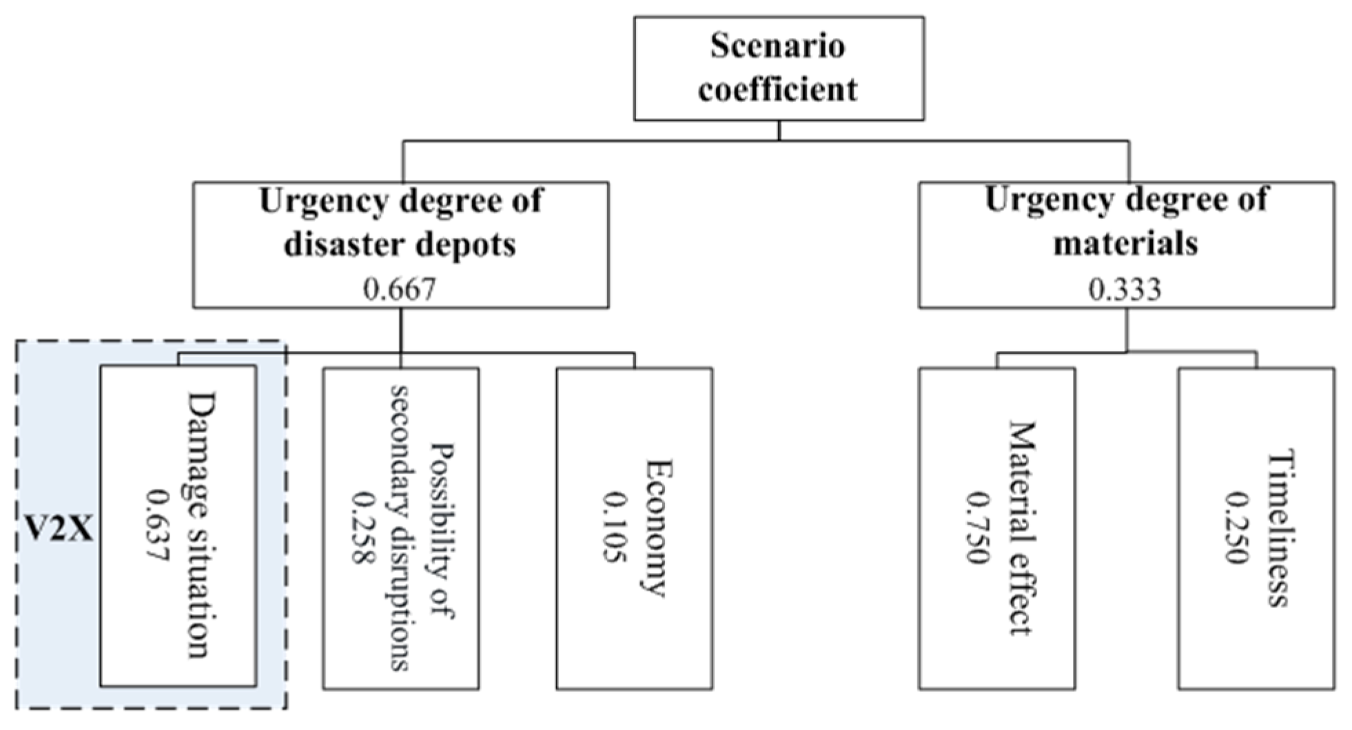
The SEMS scenario coefficient indicates the urgency of disaster demand, which mainly depends on the damage of disaster depots and the urgency of emergency materials. Here, scenario indicates some kind of emergency material that is demanded by a disaster depot. The urgency of emergency materials is determined by their role in rescue activity and time urgency in a disaster depot. Thus, we get the evaluation indicators from these two aspects. The indicators of damage situation, possibility of secondary disruptions and economy can show the urgency degree of disaster depots, and material effect and timeliness can reflect the urgency of emergency materials. The Analytic Hierarchy Process (AHP) method is used to calculate scenario coefficients. The AHP method is detailed in [28]. Figure 1 presents the architecture for defining the objective and indicators for the AHP. The top layer is the objectives layer, which evaluates the scenario coefficient. The middle layer is the rule layer, which evaluates the urgency degree of disaster depots and materials. The bottom layer is the index layer, which has five evaluation factors. The AHP method first establishes the judgment matrices through expert questionnaires, which consist of the judgment matrix O of the rule layer to the objective layer, and the judgment matrices o1 and o2 of the index layer to the rule layer. The values of the matrices were identified by expert subjective scoring according to Saaty’s 1–9 scale. We designed a questionnaire, and then collected the data from the questionnaire. These matrices are shown as O = [ 1 2 1 2 1 ] , o 1 = [ 1 3 5 1 3 1 1 4 1 5 4 1 ] , and o 2 = [ 1 3 1 3 1 ] . Table 1 presents the maximum eigenvalues, consistency indexes and consistency ratios of the three judgment matrices.
As the value of consistency ratio (C. R.) is less than 0.1, the consistency of the judgment matrices is acceptable. Table 2 presents the weight values of the weight vector.

3.2. Calculate the SEMS Transportation Time

The existing emergency material scheduling is mainly about road transportation, which ignores the preparation time of vehicles and the recovery time for damaged road repair. The SEMS takes into account both of the time and the automobile and airplane transportation in material scheduling as well.
The SEMS transportation time includes preparation time, automobile traveling time, and road repair time as Equations (1) and (2). The preparation time consists of material loading and refueling time. The road transportation time is the sum of the preparation time, automobile traveling time and road repair time. The air transportation time is the sum of the airplane preparation time and airplane traveling time. The SEMS obtains the transportation time more accurately and results in a more precise schedule by collecting real-time vehicle speeds.
t i j 1 p = t 1 + l i j 1 v 1 + l i j 1 ε i j p v 3
t i j 2 p = t 2 + l i j 2 v 2
where
  • l i j r : the distance from the supply depot i to disaster depot j with mode r . r =   1 means road transportation, and r =   2 means air transportation;
  • p : the period stage of a disaster depot for a kind of emergency material;
  • ε i j p : the road damage rate, a percentage of the damaged road between the supply depot i and disaster depot j in stage p ;
  • v 1 : the vehicle speed;
  • v 2 : the airplane speed;
  • v 3 : the road repair speed, which refers to repaired road distance per hour;
  • t 1 : the automobile preparation time, set to 0.5 h;
  • t 2 : the airplane preparation time, set to 3 h;
  • t i j 1 p : the road transportation time from i to j in stage p ;
  • t i j 2 p : the air transportation time from i to j in stage p .
Equation (1) demonstrates that the road transportation time is the sum of the automobile preparation time, traveling time and road repair time. Road damage does not exist in air transportation, so Equation (2) shows that the air transportation time is the sum of airplane preparation time and airplane traveling time. The SEMS inputs real-time vehicle speeds into the model, which obtains the transportation time more accurately, resulting in a more precise schedule.

3.3. SEMS Fairness

Fairness should be considered in emergency material scheduling, especially when the supply is insufficient. Henri Theil first noted the possibility of using Claude Shannon’s information theory to produce measures of income fairness. Later, many researchers used the Theil index to analyze the fairness and variance of fiscal expenditure, resource allocation, tourism development, etc. [29]. The SEMS chooses the Theil L index to denote fairness, which is expressed in Equation (3):
T L = k = 1 m v k ln v k u k
where TL is Theil L index, m is the number of groups, vk is the proportion of the population of group k, and uk is the proportion of the income of group k.
The Theil L index is used to show the fairness of people income among different groups. Inspired by Equation (3), we improved it to indicate the fairness of emergency material scheduling. For emergency material scheduling, we analyzed the fairness of relief distribution, so the demand satisfaction of the emergency materials of each disaster depot can be regarded as the “income” of each group in Equation (3). The scenario coefficient can reflect the basic information of each disaster depot and can be seen as “population” of each group. The following Equation (4) defines the SEMS fairness:
F = k = 1 K ( α j k p j = 1 J α j k p ln ( α j k p j = 1 J α j k p / i = 1 I r = 1 R x i j r k p / d j k p j = 1 J ( i = 1 I r = 1 R x i j r k p / d j k p ) ) )
where F is fairness, α j k p is the scenario coefficient of disaster depot j for material k in stage p , x i j r k p is the amount of material k delivered from i to j with mode r in stage p , d j k p is the actual demand for material k in disaster depot j in stage p .

3.4. SEMS Assumptions and Model

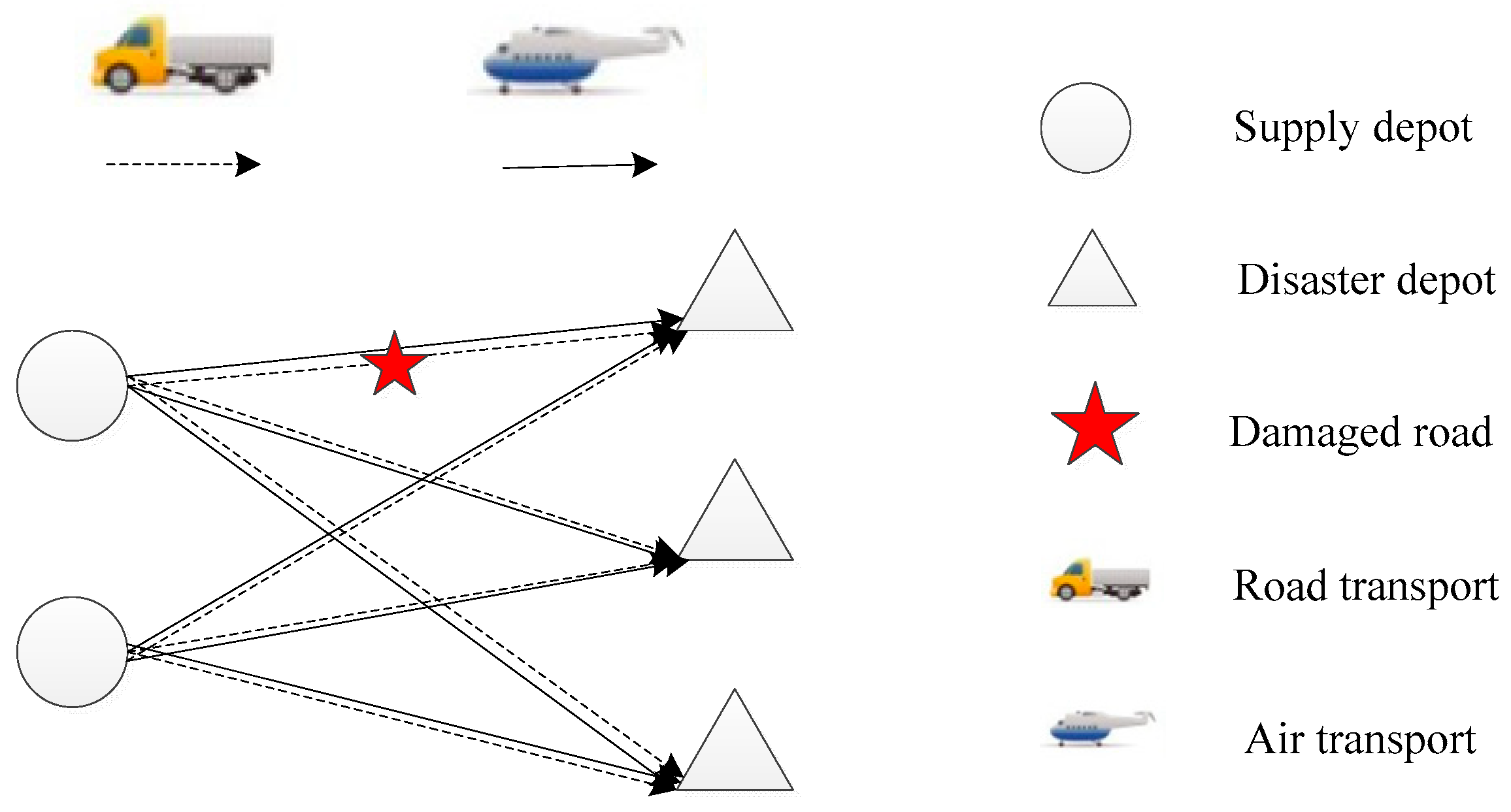
In the SEMS model, we discuss a scheduling problem of multiple supply depots, disaster depots, commodities and transport modes for logistics management of relief commodities. Transport modes include road transport and air transport. Additionally, the model considers damage to the road. The SEMS network is shown as Figure 2.

3.4.1. SEMS Assumption and Notations

We had the following assumptions for the SEMS model:
(1) The locations of supply depots and disaster depots are known;
(2) Emergency materials can only be delivered from supply depots to disaster depots;
(3) The seriously damaged emergency materials stored in disaster depots cannot be used;
(4) The amount of emergency materials stored at each supply depot is known;
(5) The scheduling time depends on the transportation mode and distance between supply depots and disaster depots;
(6) The mode selection is only made based on the transportation time, regardless of the weather and other conditions.
Table 3 defines other notations used in the paper.

3.4.2. SEMS Model

The SEMS model consists of the following fairness function and constraints:
f 1 = max k = 1 K ( α j k p j = 1 J α j k p ln ( α j k p j = 1 J α j k p / i = 1 I r = 1 R x i j r k p / d j k p j = 1 J ( i = 1 I r = 1 R x i j r k p / d j k p ) ) )
f 2 = min ( i = 1 I j = 1 J r = 1 R k = 1 K α j k p h i j r k p t i j r p )
s . t .
i = 1 I j = 1 J r = 1 R k = 1 K c r k p l i j r x i j r k p C p
j = 1 J r = 1 R h i j r k p x i j r k p =   q i k p
q i k p = q i k p 1 j = 1 J r = 1 R x i j r k p - 1 + q k n e w
d j k p = d j k p 1 i = 1 I r = 1 R x i j r k p - 1 + d k n e w
h i j r k p = { 0 , x i j r k p = 0 1 , x i j r k p 0
Equation (5) maximizes the SEMS fairness of material scheduling, whereas Function (6) minimizes the SEMS transportation time. Constraint (7) ensures that the total transportation cost does not exceed the available budget. Constraint (8) indicates that the sum of all supply depots is equal to their storage. Constraint (9) indicates that the supply in stage p is the sum of the remaining in stage p 1 and the supply generated in stage p . Similarly, Constraint (10) states that the demand in stage p is the sum of a new demand generated in stage p and the demand not met in stage p 1 .

3.5. SEMS Algorithm

The Artificial Fish-Swarm Algorithm (AFSA) is one of the swarm intelligence algorithms. It consists of a population of fishes interacting locally with one another and their environment by following rules. This algorithm has the advantages of high convergence speed, flexibility, fault tolerance and high accuracy [30].
There are many swarm intelligence algorithms, such as particle swarm optimization (PSO), ant colony optimization (ACO), and bacterial foraging optimization (BFO). Particle swarm optimization is inspired by the social behavior among individuals, for instance, bird flocks. Particles representing a potential solution to the optimization problem move through a search space. Particle swarm optimization comprises a very simple concept, and paradigms can be implemented in a few lines of computer code [31,32]. It requires only primitive mathematical operators, and is computationally inexpensive in terms of both memory requirements and speed. However, its disadvantage is premature convergence that leads to a fall into local optimum. Moreover, the values of parameters affect the operation of PSO greatly. Ant colony optimization was inspired by observations of the foraging behavior of real ants, which is applied to solve discrete combinatorial optimization problems [33]. The ants leave pheromone while traveling. The intensity of pheromone governs the movement of the whole ant community. Subsequently, pheromone intensity becomes very high along the shortest path, and finally all ants will converge to the food. The convergence speed of ACO is relatively slow because the pheromone intensity is basically the same in the beginning and gradually the path with a higher pheromone intensity will be found, which will waste much time in the initial stage of computation. Local optimum is also a problem for ACO.
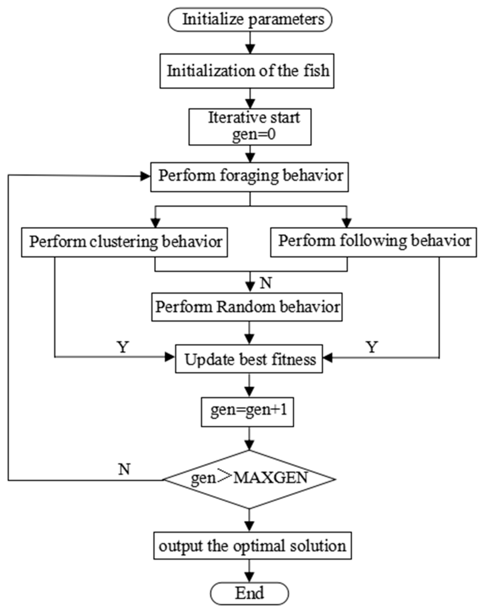
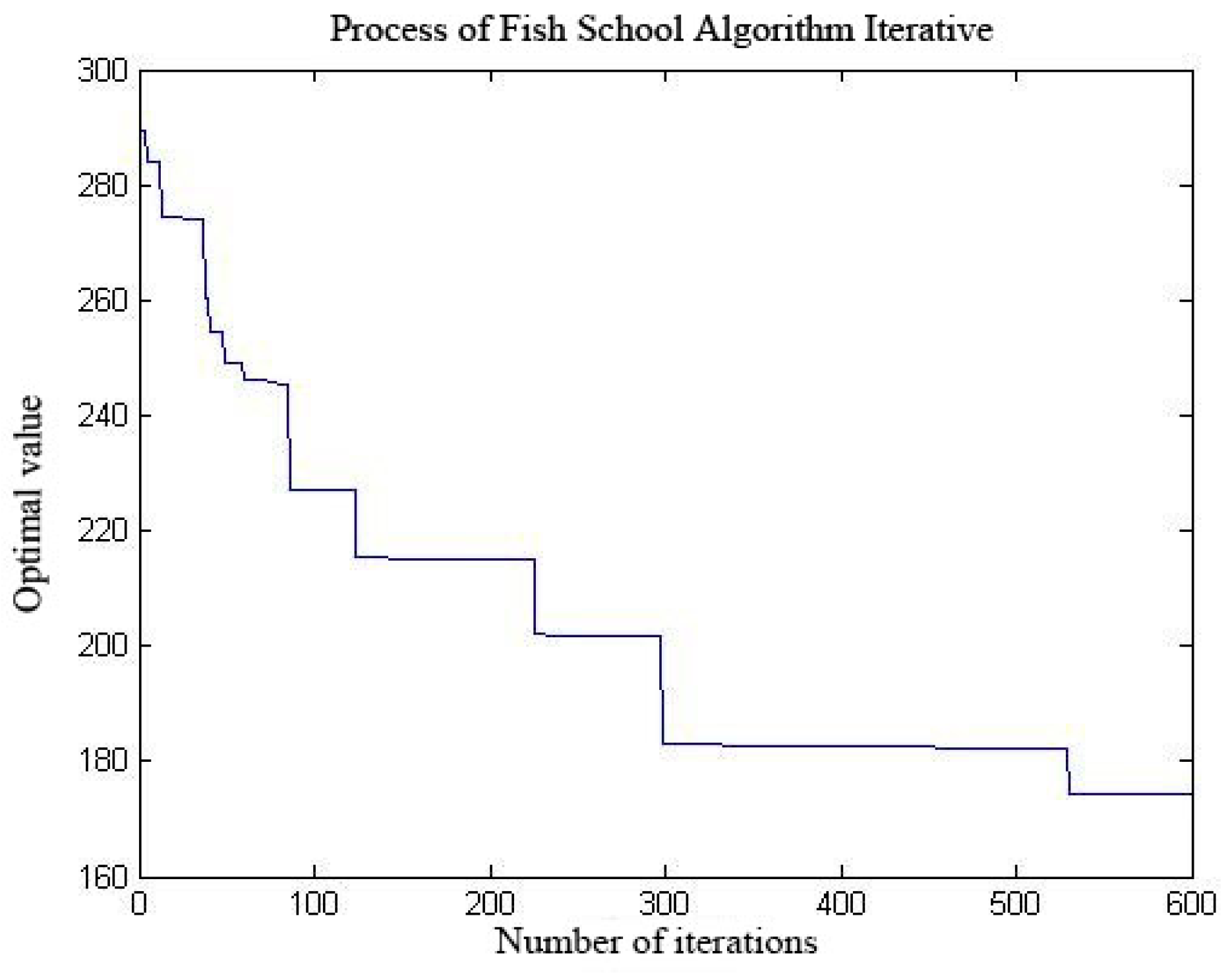
After a disaster occurs, emergency material scheduling is very urgent. Thus, we need an algorithm with a high searching speed. The AFSA has a high convergence speed. Moreover, to solve the problem of local optimum, congestion factor is introduced into the AFSA. Congestion factor is an important parameter to constrain the excessive clustering behavior of fishes, which can avoid local optimum effectively. Therefore, we designed the SEMS algorithm based on the AFSA according to the following steps. The SEMS takes fairness as the main objective and transport time as the secondary objective.
Step 1: Set parameters, including the fishes scale—fish num, the maximum number of foraging trials—try_number, the fish group perception distance—visual, the crowd factor delta, the moving step length—step, and the maximum iteration number—MAXGEN;
Step 2: Artificial fish coding. Individual fishes are coded with real numbers and expressed as a matrix. Each artificial fish represents a plan for emergency material scheduling;
Step 3: Initialization of the fishes. The current iteration number gen = 0. If the supply depot participates in a plan, the supply of emergency materials is a random positive number less than or equal to the storage amount, otherwise it is 0;
Step 4: Evaluation of the fitness of each fish by performing foraging. This step is to solve the objective function, that is, to find the maximum fairness and minimum time while meeting the constraints;
Step 5: Update the fitness by performing clustering and following behaviors. Each artificial fish performs clustering and following behaviors individually. If the existing value is optimal, it becomes the new optimal value, otherwise the fish continues foraging;
Step 6: Check whether it reaches the maximum iteration number, MAXGEN. If yes, it outputs the optimal value, otherwise the variable gen adds one and the algorithm goes to step 3.
The SEMS algorithm is illustrated in Figure 3.

4. Experiment

The Wenchuan earthquake occurred in Sichuan Province, China on 12 May 2008 at 8.0 Richter scale, killing 69,227 people and injuring 374,643 people. Gauze, tents and water were dispatched from Xi’an and Lanzhou to Chengdu, Shifang and Jiangyou during the disaster. The disaster and supply depots are shown in Figure 4. The distances between the depots are shown in Table 6.

4.1. Scenario Coefficient

We calculated the scenario coefficients based on the SEMS evaluation indicators and the AHP method with the data collected by V2X communications and data from the websites [34,35]. The scenario coefficients for Chengdu’s, Shifang’s and Jiangyou’s demand for gauze, tents and water are 0.095, 0.057, 0.064, 0.195, 0.157, 0.165, 0.112, 0.074 and 0.081, respectively.

4.2. Parameters

Table 4 presents the cost for delivering 10,000 pieces of material per kilometer, which includes fuel and labor costs.
Table 5 presents the road damage rate between the supply depots and the disaster depots.
According to [36], road repair speed is 0.5 km/h. It was assumed that the speed of vehicle and airplane are 100 and 200 km/h, respectively; the preparation time for automobile and airplane are 0.5 and 3 h, respectively, based on the investigation of logistics centers and military airports in China. With V2X communications, the real-time vehicle speed can be acquired and updated in the SEMS model. Table 6 and Table 7 present the shortest transportation distances and minimum transportation time based on the parameters above.
It was assumed that the budget for the emergency material scheduling was 80 million RMB.
Table 8 presents the relief demand for each disaster depot, where a box of water is 12 bottles. Table 9 presents the relief amount for each supply depot.

4.2.1. Fairness Analysis

The proposed SEMS model includes two objectives, i.e., maximum fairness and minimum time, which are solved by a hierarchical sequence method. We took fairness as the main objective and transport time as the secondary objective. First, the fairness model was solved with MATLAB. Table 10 presents the used parameters.
Figure 5 presents the iteration curve for optimizing the SEMS fairness. Table 11 presents the scheduling plan with the maximum fairness. In Figure 5, the x-axis represents the number of iterations, and the y-axis represents the optimized value of fairness. Thus, the unit for the x-axis is time. It is the same in Figure 6, Figure 7, Figure 8 and Figure 9.
The abbreviation Amt denotes the amount of relief demand, and Sat Rate denotes the demand satisfaction rate of the disaster depots.
To prove the priority of the SEMS model, we compared it with the Gini index fairness model (Gini model) in [21] using the AFSA. The related results of the Gini model are given in Figure 6 and Table 12.
Similarly, we also compared the SEMS with the enhanced Theil fairness model (enhanced Theil model) as Equation (12). The related results of the enhanced Theil model are shown in Figure 7 and Table 13.
F = j = 1 J k = 1 K α j k p j = 1 J k = 1 K α j k p ln ( α j k p j = 1 J k = 1 K α j k p / x i j r k p i = 1 I j = 1 J k = 1 K x i j r k p )
where F is fairness of the enhanced Theil model; α j k p and x i j r k p are defined in Equation (4).
Thus, we compared the scheduling plan with the maximum SEMS fairness, the Gini model and the enhanced Theil model, and then made the following conclusions based on Table 11, Table 12 and Table 13:
(1). Comparison between the Gini model and SEMS model.
As shown in Table 8, the tent demand for Jiangyou is 149, Shifang 4462, and Chengdu 10,993. The tent demand for Jiangyou is very small and that for Chengdu is large. As shown in Table 12, the optimized solution to the Gini model ignores the demand for Jiangyou and its scheduling amount and demand satisfaction rate are both 0. In the Gini model, for Shifang, the tent demand satisfaction rate is only 0.4281. However, that of the SEMS model is 0.9620. For Chengdu the tent demand satisfaction rate is 0.9187, whereas it is 0.6644 in the SEMS model. This states that the Gini model only meets the disaster depots with a high demand, while ignoring the depots with low demand, although the SEMS model can provide a fairer solution. Table 11 presents the optimized SEMS solution, where the demand satisfaction rate of Jiangyou attains 0.8187, and that of Shifang is 0.9620. Compared with the Gini model, the SEMS considers the disaster depots with low demand. Even though the demand for some material of a disaster depot is very low, it can still receive some emergency materials when the relief supplies are insufficient.
(2). Comparison between the enhanced Theil model and SEMS model.
As shown in Table 8, the tent demand for Chengdu is higher than Shifang, whereas the scenario coefficient for Chengdu is 0.057, less than that of Shifang 0.157. It means the tent demand for Shifang is more urgent than that for Chengdu. As shown in Table 11, the demand satisfaction rate for Chengdu is 0.6644 in the SEMS model, and lower than that of Shifang 0.9620, whereas the enhanced Theil model is the opposite. Therefore, the SEMS model considers the urgency of emergency material for disaster depots and can guarantee the demand with a high scenario coefficient, so it is closer to the actual situation.
In summary, compared with the Gini model and the enhanced Theil model, the proposed SEMS model considers the low demand for disaster depots and guarantees the emergency materials with a high scenario coefficient.

4.2.2. SEMS Scheduling Time

Based on the optimized solution for maximum fairness, the SEMS algorithm was used to obtain the optimized scheduling time. Table 14 presents the used parameters.
The iterative curve for the SEMS scheduling time optimization is shown in Figure 8, and the SEMS scheduling plan is shown in Table 15.
We compared the SEMS with the enhanced Theil model, whose optimal objective for the scheduling time is expressed as Equation (13):
f 2 = min r = 1 R i = 1 I j = 1 J h i j r p t i j r p
The related results of the enhanced Theil model are shown in Figure 9 and Table 16.
Similarly, Table 17 compares the optimized scheduling time obtained by the SEMS model and the enhanced Theil model.
Thus, we compared the optimized scheduling time between the SEMS model and the enhanced Theil model, and then made the following conclusions based on Table 17.
As shown in Figure 8, the optimized scheduling time by the SEMS model is 28.180 h. We applied the same solution to the enhanced Theil model, and obtained the total scheduling time of 168.190 h. As shown in Figure 9, the optimized solution for the enhanced Theil model is 165.850 h. The total scheduling time achieved by the SEMS and the enhanced Theil model are similar, which shows that the SEMS scheduling time optimization is feasible with the consideration of the scenario coefficient.
If the scenario coefficient of emergency material is larger, the emergency material should be delivered to the disaster depot earlier. In the optimized SEMS solution, the scheduling time of emergency material with a larger scenario coefficient is shorter, whereas the enhanced Theil model does not obey this rule.
Take Shifang, for example: the scenario coefficient of gauze is more than that of tents, and in the SEMS model the scheduling time of gauze (6.370 h) is much shorter than that of tents (14.100 h). The enhanced Theil model gives an opposite answer, where the scheduling time of gauze is 19.650 h and that of tents is 18.500 h. The reason is that the scenario coefficient of gauze is larger than that of tents, which indicates that the gauze demand is more urgent than the demand for tents. Taking Chengdu as another example, the scenario coefficient of gauze is more than that of tents, and in the SEMS model the scheduling time of gauze (5.725 h) is much shorter than that of tents (17.955 h), whereas in the enhanced Theil model, the scheduling time of gauze is more than that of tents. Thus, compared with the enhanced Theil model, the proposed SEMS model guarantees faster delivery of relief with a higher scenario coefficient. Thus, the SMES model is more in line with the actual situation.

5. Conclusions and Future Work

Point-to-point V2X provides us with a new way of studying the existing emergency material distribution problem. With V2X, more dynamic data of vehicles and information of disaster scenarios can be acquired, which will help decision-makers plan relief logistics scientifically. The V2X communications present a golden opportunity for real-time, precise emergency material scheduling. We introduced the SEMS with the use of V2X communications. A scenario coefficient was introduced into the modeling of emergency material scheduling. We used point-to-point V2X communication to identify the values of the scenario coefficient. The SEMS model takes into account the urgency of disaster scenarios and enhances the fairness for relief scheduling, which outperforms the Gini model and enhanced Theil models. The research provides a more comprehensive method to make an emergency material scheduling plan and reminds us that the delivery of emergency material should consider the actual situation of disaster depots, such as damage to disaster depots and secondary disaster. The modeling will also evolve with the development of technology, such as tools for collecting data and the technique of data processing.
Nevertheless, there is still great potential for improving the performance of emergency material scheduling. First, in the evaluation of the scenario coefficient, the urgency degree of disaster areas and materials was considered; however, the evaluation indicators and their weights should be analyzed further. A more objective method should be introduced and designed to calculate the scenario coefficient. Secondly, the road damage rate was assumed to be a fixed value, whereas emergencies are usually accompanied with the secondary emergencies which may also destroy the road again. Therefore, the road damage rate should also be updated to real time. Finally, inspired by the mobile app called Earthquake Quick Report by GeTui, a big data provider in China, big data have also been applied to help in emergency rescue. With the help of such tools, we can get data more quickly and precisely, which will enhance the demand forecasting accuracy. Moreover, after related information including vehicle position, damage to the roads, and surrounding environment are collected via V2X, how to standardize the data in various formats (digit and video) scientifically is also a challenging direction in the future.

Author Contributions

H.H. is the main author of this article. She designed the experiment, constructed the main structure of this paper and was responsible for modeling. K.C. was in charge of the case study. J.H. collected relevant data and contributed to data analysis. Y.Z. was responsible for the result analysis and conclusion. J.Z. verified the validity of the model and put forward some suggestions for improving the model and writing. Y.H. contributed to the paper’s modification and refinement. All the authors read and approved the final manuscript.

Funding

This research was supported by the National Natural Science Foundation of China under Grant U1664264, the China Fundamental Research Funds for the Central Universities under Grant 3100102229103 and 300102229111, Xi’an Social Science Planning Fund under Grant 19Z73 and the China Innovation and Entrepreneurship Training Program for College Students under Grant 20191071245.

Conflicts of Interest

The authors declare no conflict of interest.

References

  1. Sheu, J.B. An emergency logistics distribution approach for quick response to urgent relief demand in disasters. Transp. Res. Part E Logist. Transp. Rev. 2007, 43, 687–709. [Google Scholar] [CrossRef]
  2. Sheu, J.B.; Pan, C. Relief supply collaboration for emergency logistics responses to large-scale disasters. Transp. A Transp. Sci. 2015, 11, 210–242. [Google Scholar] [CrossRef]
  3. Rachida, A.; Monia, R.; Jacques, R. An exact solution approach for multi-objective location transportation problem for disaster response. Comput. Oper. Res. 2014, 41, 83–93. [Google Scholar]
  4. Kokuti, A.; Hussein, A.; Marin-Plaza, P.; de la Escalera, A.; García, F. V2X communications architecture for off-road autonomous vehicles. In Proceedings of the 2017 IEEE International Conference on Vehicular Electronics and Safety (ICVES), Vienna, Austria, 27–28 June 2017. [Google Scholar]
  5. Vukadinovic, V.; Bakowski, K.; Marsch, P. 3GPP C-V2X and IEEE 802.11p for Vehicle-to-Vehicle communications in highway platooning scenarios. Ad Hoc Netw. 2018, 74, 17–29. [Google Scholar] [CrossRef]
  6. Machardy, Z.; Khan, A.; Obana, K. V2X Access technologies: Regulation, research, and remaining challenges. IEEE Commun. Surv. Tut. 2018, 20, 1858–1877. [Google Scholar] [CrossRef]
  7. Özdamar, L.; Ekinci, E.; Küçükyazici, B. Emergency logistics planning in natural disasters. Ann. Oper. Res. 2004, 129, 217–245. [Google Scholar]
  8. Sebbah, S.; Boukhtouta, A.; Berger, J.; Ghanmi, A. Military Logistics Planning in Humanitarian Relief Operations. In Humanitarian and Relief Logistics; Springer: New York, NY, USA, 2013; pp. 77–110. [Google Scholar]
  9. Safeer, M.; Anbuudayasankar, S.P.; Balkumar, K.; Ganesh, K. Analyzing transportation and distribution in emergency humanitarian logistics. Procedia Eng. 2014, 97, 2248–2258. [Google Scholar] [CrossRef]
  10. Hamedi, M.; Haghani, A.; Yang, S. Reliable Transportation of Humanitarian Supplies in Disaster Response: Model and Heuristic. Procedia Soc. Behav. Sci. 2012, 54, 1205–1219. [Google Scholar] [CrossRef] [Green Version]
  11. Ferrer, J.M.; Martín-Campo, F.J.; Ortuño, M.T.; Pedraza-Martínez, A.J.; Tirado, G.; Vitoriano, B. Multi-criteria optimization for last mile distribution of disaster relief aid: Test cases and applications. Eur. J. Oper. Res. 2018, 269, 501–515. [Google Scholar] [CrossRef]
  12. Ahmadi, M.; Seifi, A.; Tootooni, B. A humanitarian logistics model for disaster relief operation considering network failure and standard relief time: A case study on San Francisco district. Transp. Res. Part E Logist. Transp. Rev. 2015, 75, 145–163. [Google Scholar] [CrossRef]
  13. Owusu-Kwateng, K.; Abdul, H.M.; Debrah, B. Disaster relief logistics operation: An insight from Ghana. Int. J. Emerg. Serv. 2017, 6, 4–13. [Google Scholar] [CrossRef]
  14. Rahafrooz, M.; Alinaghian, M. A novel robust chance constrained possibilistic programming model for disaster relief logistics under uncertainty. Int. J. Ind. Eng. Comput. 2016, 7, 649–670. [Google Scholar] [CrossRef]
  15. Rachaniotis, N.P.; Dasaklis, T.; Pappis, C.P.; Van Wassenhove, L.N. Multiple location and routing models in humanitarian logistics. In Humanitarian and Relief Logistics; Springer: New York, NY, USA, 2013; pp. 43–57. [Google Scholar]
  16. Lu, C.C.; Sheu, J.B. Robust vertex p-center model for locating urgent relief distribution centers. Comput. Oper. Res. 2013, 40, 2128–2137. [Google Scholar] [CrossRef]
  17. Najafi, M.; Eshghi, K.; Dullaert, W. A multi-objective robust optimization model for logistics planning in the earthquake response phase. Transp. Res. Part E Logist. Transp. Rev. 2013, 49, 217–249. [Google Scholar] [CrossRef]
  18. Ransikarbum, K.; Mason, S.J. Goal programming-based post-disaster decision making for integrated relief distribution and early-stage network restoration. Int. J. Prod. Econ. 2016, 182, 324–341. [Google Scholar] [CrossRef]
  19. Liu, C.; Zeng, Q.; Duan, H.; Zhou, M.; Lu, F.; Cheng, J. E-Net modeling and analysis of emergency response processes constrained by resources and uncertain durations. IEEE Trans. Syst. Man Cybern. 2015, 45, 84–96. [Google Scholar]
  20. Bozorgi-Amiri, A.; Jabalameli, M.S.; Al-E-Hashem, S.M. A multi-objective robust stochastic programming model for disaster relief logistics under uncertainty. OR Spectr. 2013, 35, 905–933. [Google Scholar] [CrossRef]
  21. Liu, J.Y. Study on Route Optimal Allocation Method of Flood Disaster Emergency Rescue Materials. Master’s Thesis, Shenyang University, Shenyang, China, 2017. [Google Scholar]
  22. Chen, L.L. Optimal scheduling model for emergency logistics based on satisfaction under large-scale emergencies. China Saf. Sci. J. 2010, 20, 46–52. [Google Scholar]
  23. Kostreva, M.M.; Ogryczak, W.; Wierzbicki, A. Equitable aggregations and multiple criteria analysis. J. Oper. Res. 2004, 158, 362–377. [Google Scholar] [CrossRef] [Green Version]
  24. Chang, F.S.; Wu, J.S.; Lee, C.N.; Shen, H.C. Greedy-search-based multi-objective genetic algorithm for emergency logistics scheduling. Expert Syst. Appl. 2014, 41, 2947–2956. [Google Scholar] [CrossRef]
  25. Han, Y.; Xue, N.N.; Wang, B.Y.; Zhang, Q.; Liu, C.L.; Zhang, W.S. Improved dual-protected ring signature for security and privacy of vehicular communications in vehicular Ad-hoc networks. IEEE Access 2018, 6, 20209–20220. [Google Scholar] [CrossRef]
  26. Zhang, W.; Xu, L.; Li, Z.; Lu, Q.; Liu, Y. A Deep-Intelligence Framework for Online Video Processing. IEEE Softw. 2016, 33, 44–51. [Google Scholar] [CrossRef]
  27. Feng, J.; Liu, Z.; Wu, C.; Ji, Y. AVE: Autonomous Vehicular Edge computing framework with ACO-based scheduling. IEEE Trans. Veh. Technol. 2017, 66, 10660–10675. [Google Scholar] [CrossRef]
  28. Saaty, T.L. Decision-making with the AHP: Why is the principal eigenvector necessary. Eur. J. Oper. Res. 2003, 145, 85–91. [Google Scholar] [CrossRef]
  29. Almeida, R.K.; Carneiro, P. Inequality and Employment in a Dual Economy: Enforcement of Labor Regulation in Brazil; Social Science Electronic Publishing: Rochester, NY, USA, 2017. [Google Scholar]
  30. Neshat, M.; Sepidnam, G.; Sargolzaei, M.; Toosi, A.N. Artificial fish swarm algorithm: A survey of the state-of-the-art, hybridization, combinatorial and indicative applications. Artif. Intell. Rev. 2014, 42, 965–997. [Google Scholar] [CrossRef]
  31. Kennedy, J.; Eberhart, R. Particle Swarm Optimization. In Proceedings of the 1995 IEEE International Conference on Neural Networks, Perth, WA, Australia, 27 November–1 December 1995. [Google Scholar]
  32. Huang, C.L.; Huang, W.C.; Chang, H.Y. Hybridization strategies for continuous ant colony optimization and particle swarm optimization applied to data clustering. Appl. Soft Comput. 2013, 13, 3864–3872. [Google Scholar] [CrossRef]
  33. Raj, U.; Mulani, K.; Talukdar, P.; Das, A. Performance analysis and feasibility study of ant colony optimization, particle swarm optimization and cuckoo search algorithms for inverse heat transfer problems. Int. J. Heat Mass Transf. 2015, 89, 359–378. [Google Scholar]
  34. People.cn. Available online: http://society.people.com.cn/GB/8217/7241096.html?z=nck4y1jgj991teju (accessed on 8 May 2019).
  35. The General Office of the State Council. Available online: http://www.gov.cn/zwgk/2010-06/13/content_1626853.htm (accessed on 23 April 2019).
  36. Li, S.L.; Teo, K.L. Post-disaster multi-period road network repair: Work scheduling and relief logistics optimization. Ann. Oper. Res. 2018, 1–41. [Google Scholar] [CrossRef]
Figure 1. Evaluation indicators for the scenario-based approach for emergency material scheduling (SEMS) scenario coefficient.
Electronics 08 00707 g001
Figure 2. SEMS network.
Electronics 08 00707 g002
Figure 3. The SEMS algorithm.
Electronics 08 00707 g003
Figure 4. Disaster and supply depots in the Wenchuan earthquake.
Electronics 08 00707 g004
Figure 5. Iteration curve for SEMS fairness optimization.
Electronics 08 00707 g005
Figure 6. Iterative curve for the Gini model optimization.
Electronics 08 00707 g006
Figure 7. Iterative curve for the enhanced Theil fairness optimization.
Electronics 08 00707 g007
Figure 8. Iterative curve for SEMS scheduling time optimization.
Electronics 08 00707 g008
Figure 9. Iterative curve for the enhanced Theil scheduling time optimization.
Electronics 08 00707 g009
Table 1. Maximum eigenvalues, consistency index (C. I.) and consistency ratio (C. R.).
Maximum EigenvaluesC. I.C. R.
O200
O13.03370.0200.034
O2200
Table 2. Values of the weight vector.
ω
O(0.667, 0.333)
O1(0.637, 0.258, 0.105)
O2(0.750, 0.250)
Table 3. Definition of notations.
NotationsMeaning
q i k p The supply amount of material k stored in depot i in stage p
q k n e w The supply amount of material k generated in stage p
d k n e w The demand of material k generated in stage p
c r k p The transportation cost for dispatching k using mode r in stage p
l i j r The distance from the supply depot i to j with mode r
C p The total emergency cost raised in stage p
h i j r k p Whether or not dispatching k from depot i to j by mode r in stage p
θ p The saving index of an emergency material in stage p , which changes with the stage advancement
x i j r k p The amount of material dispatching k from depot i to j by mode r in stage p
α j k p The scenario coefficient of disaster depot j for material k in stage p
d j k p The actual demand for material k in disaster depot j in stage p
Table 4. Delivery cost. Key: G represents gauze, T represents tents and W represents water.
ModeG/YuanT/YuanW/Yuan
Road300010,0007000
Air10,00020,00012,000
Table 5. Road damage rate.
ChengduShifangJiangyou
Xi’an1%2%3%
Lanzhou3%2%1%
Table 6. Shortest transportation distance between depots.
ItemChengduShifangJiangyou
Xi’anRoad distance/km726680585
Flight distance/km545510439
LanzhouRoad distance/km950900823
Flight distance/km713675617
Table 7. The minimum transportation time between depots.
ItemChengduShifangJiangyou
Xi’anRoad/h11.39014.10015.125
Air/h5.7255.5505.195
LanzhouRoad/h24.25018.50012.845
Air/h6.5656.3756.085
Table 8. Relief demand for each disaster depot.
MaterialChengduShifangJiangyou
G/Packages573510,0007750
T/Tops10,9934462149
W/Boxes18,48754,19612,260
Table 9. Relief demand for amount for each supply depot.
MaterialXi’anLanzhou
G/Packages10,00010,000
T/Tops60006000
W/Boxes40,00040,000
Table 10. Parameters used in the SEMS algorithm.
Fish NumberMaximum Number of IterationsMaximum Number of TrialsPerceived DistanceCongestion FactorStep Distance
30800500.0110.1
Table 11. Scheduling plan with maximum fairness.
ChengduShifangJiangyou
GTWGTWGTW
Amt4165730415,4349165429353,169667212210,873
Sat Rate0.72620.66440.83480.91650.96200.98100.86080.81870.8869
Table 12. Scheduling plan for the Gini model.
ItemChengduShifangJiangyou
GTWGTWGTW
Amt374410,10017,3249701191052,5786643010,276
Sat Rate0.65280.91870.93710.97010.42810.97010.857200.8382
Table 13. Scheduling plan for enhanced Theil model.
ItemChengduShifangJiangyou
GTWGTWGTW
Amt3517899316,48810,031300852,39165141009952
Sat Rate0.61330.81800.89191.00310.67410.96670.84050.67110.8117
Table 14. Parameters used in the SEMS algorithm.
Fish NumberMaximum Number of IterationsMaximum Number of TrialsPerceived DistanceCongestion FactorStep Length
30600500.0110.1
Table 15. The SEMS scheduling plan.
ModeChengduShifangJiangyou
GTWGTWGTW
Xi’anRoad0201400403412,810447003261
Air42960109800393301000
LanzhouRoad0000012,369177502600
Air0512960768650022,088004763
Table 16. Scheduling plan for the enhanced Theil model.
ModeChengduShifangJiangyou
GTWGTWGTW
Xi’anRoad0029833999032,117000
Air06862560241360044511220
LanzhouRoad450902755042330005648
Air0038390017,957005244
Table 17. Comparison of the optimized scheduling time.
ModelChengduShifangJiangyou
GTWGTWGTW
SEMS model/Hour5.72517.95512.2906.37014.10044.52527.9705.19534.055
Enhanced Theil model/Hour24.2505.72547.93019.65018.50020.4755.1955.19518.930

