Multi-Branch Spectral Channel Attention Network for Breast Cancer Histopathology Image Classification

Abstract

Deep-learning-based breast cancer image diagnosis is currently a prominent and growingly popular area of research. Existing convolutional-neural-network-related methods mainly capture breast cancer image features based on spatial domain characteristics for classification. However, according to digital signal processing theory, texture images usually contain repeated patterns and structures, which appear as intense energy at specific frequencies in the frequency domain. Motivated by this, we make an attempt to explore a breast cancer histopathology classification application in the frequency domain and further propose a novel multi-branch spectral channel attention network, i.e., the MbsCANet. It expands the interaction of frequency domain attention mechanisms from a multi-branch perspective via combining the lowest frequency features with selected high frequency information from two-dimensional discrete cosine transform, thus preventing the loss of phase information and gaining richer context information for classification. We thoroughly evaluate and analyze the MbsCANet on the publicly accessible BreakHis breast cancer histopathology dataset. It respectively achieves the optimal image-level and patient-level classification results of 99.01% and 98.87%, averagely outperforming the spatial-domain-dominated models by a large margin, and visualization results also demonstrate the effectiveness of the MbsCANet for this medical image application.

1. Introduction

Breast cancer is the leading cause of morbidity and mortality among female cancers. In 2020, 19.29 million new cancer cases were reported worldwide, and 2.29 million of them were breast cancer cases [1]. Meanwhile, breast cancer accounts for 15.5 percent of the 4.4 million female cancer-related deaths. While early diagnosis and treatment are particularly vital to improve the survival rate of cancer patients, biopsy analysis is the gold standard in the diagnosis of breast cancer. However, manual biopsy analysis is time-consuming, and the results are generally influenced by subjective factors. With the increasing number of cancer patients, computer-assisted breast cancer biopsy analysis has become more and more popular.

Recently, deep learning has made tremendous progress in a variety of computer vision and medical image analysis tasks. Consequently, convolutional neural network (CNN)-related models are attracting much attention in breast cancer histopathology image classification [2,3,4] and display obvious superiority to previous methods with accuracy that is nearly similar to or better than human experts. These works above indicate that computer-assisted technologies based on CNNs are helpful for diagnosing cancer and thus deserve further exploration. Until now, the intention of various CNN-based models has been to extract deep convolutional features, as CNNs pretrained on large-scale datasets [5,6] provide more general features despite not being trained on corresponding, specific breast cancer datasets from scratch. However, naive feature extraction from CNNs without extra personalized modeling usually omits useful, related responses from the regions of interest. The characteristics of potential regions of interest, such as nuclei, mitotic cells, and glands, are significantly critical for judging the degree of malignancy of tumors. Therefore, ignoring these features (parts of the potential region of interest) may change the final diagnostic results. This has motivated researchers to introduce attention mechanisms into computer vision systems for improving their performance by highlighting vital features. In vision systems, the attention mechanism can be thought of as a dynamic selection process that is implemented by adaptively weighting features according to the importance of the input. Hu et al. [7] first introduced the concept of channel attention and proposed the SENet built upon CNN models. SENet utilizes a means to represent each channel via global average pooling (GAP) and adaptively captures the potential key channel features according to the importance among all channels using fully connected layers and a sigmoid activation function. CBAM [8] and ECANet [9] are representative works of this kind of attention. CBAM extends SENet by introducing extra global max pooling to the channel direction to represent the associated channel. ECANet improves SENet from the view of efficiency, and a one-dimensional convolution layer with negligible parameters is adopted to replace the fully connected one to reduce the redundancy. The most recent works [10,11,12,13,14] employing a vision transformer (ViT) [15] also follow the attention mechanism.

In the field of histopathology image classification, hematoxylin and eosin (H&E) is a common staining method for biopsy images to detect the microstructure of the image to grade and stage the tissue [16], but such images have the problems of low contrast and highly variable appearance [17]. At the same time, the noise, brightness, and texture changes in high-resolution images make the depth learning model face challenges in image classification. Thus, frequency analysis, as a strong tool in the signal processing field, may be an effective and potential solution to this task in practical applications. In addition, some works exploring applications for frequency analysis in various tasks emerge as well. In [18], the authors train CNNs by JPEG encoding and decompress a blockwise frequency representation to an expanded pixel representation. Ehrlich et al. [19] propose a model conversion algorithm to convert the spatial-domain CNN models to the frequency domain and show faster training and inference speed. In [20], the discrete cosine transform (DCT) domain (or frequency domain) is incorporated into CNNs, which can reduce the communication bandwidth and better preserve image information. Dziedzic et al. [21] constrain the frequency spectra of CNN kernels to reduce memory consumption. Spectral diffusion [22] is also proposed for image generation tasks, where spectrum dynamic denoising is performed with the wavelet gating operation and thus enhances the frequency bands.

The studies above introduce frequency domain analysis into CNN-related models, but the effects on different frequency domain components are not taken into account, especially when combined with the effective channel attention mentioned above (e.g., SENet). Generally speaking, more valuable information will be more concentrated in the low-frequency area. Previous work [23] points out that GAP is mostly utilized in the existing channel attention methods, such as SENet and ECANet, to compactly compress channels so that they can be merely equivalent to the lowest frequency components of discrete cosine transform despite their motivations not being formulated from this view. Due to the effectiveness and competitiveness of channel attention, in addition to the lowest frequency components, components from other unexplored frequencies deserve further excavation and attention. As the first work introducing frequency analysis into channel attention, the frequency channel attention network (FcaNet) [23] represents channels using discrete cosine transform (DCT) instead of the lowest frequency component, i.e., GAP. Given a feature map, FcaNet splits it into many parts along channel dimension and mines multiple frequency components of 2D DCT to represent channels in each part. Lai et al. [24] introduced a novel mixed attention network (MAN) for hyperspectral image denoising. This approach overcomes previous limitations by simultaneously addressing inter- and intra-spectral correlations and feature interactions. Utilizing a multi-head recurrent spectral attention mechanism, progressive spectral channel attention, and an attentive skip connection, MAN outperforms existing methods in both simulated and real noise conditions, with efficiency in parameters and running time. Therefore, we advocate the channel attention mechanism that guides the network to focus on different frequency domains of the images, rationally distributing attention to low-frequency and high-frequency information. In this way, the network will learn the underlying patterns and will focus its attention on the valuable components in the frequency domain, thus obtaining rich context.

Further, we reexamine the existing frequency attention mechanism and propose a new multi-branch frequency attention mechanism from the frequency perspective. Our work designs a novel multi-branch spectral channel attention network, i.e., the MbsCANet, which consists of stacked MbsCA blocks. Its overall pipeline is shown in Figure 1. The proposed MbsCA block extends the original channel attention structure in SENet and FcaNet from a single branch to multiple branches, whose structure is illustrated in Figure 2. In each branch, we mine one frequency component of DCT and utilize it to represent all channels. Then, the frequency component is passed through fully connected layers to predict the weights of channels, and such weights are used to scale the corresponding channels. In all branches, different frequency components are considered to represent channels and predict channel weights for scaling. There are significant differences between ours and SENet or FcaNet. SENet is a single-branch structure and only employs the lowest frequency components (i.e., GAP) to represent channels. It is a special and simple case of ours. As for FcaNet, it is a single-branch structure as well. It uniformly divides channels into groups and each single grouped channel is represented by one frequency component. Differently, ours does not need to group channels, and each channel is represented by the multiple frequency components of DCT via a multi-branch structure. And the experiment’s results demonstrate that our method achieves better performance against both of them.

The paper makes the following contributions:

(1)

We analyze the characteristics and attention mechanism of pathological tissue images of breast cancer from the perspective of frequencies. Following this view, we design a new channel attention network, the MbsCANet, in the frequency domain.

(2)

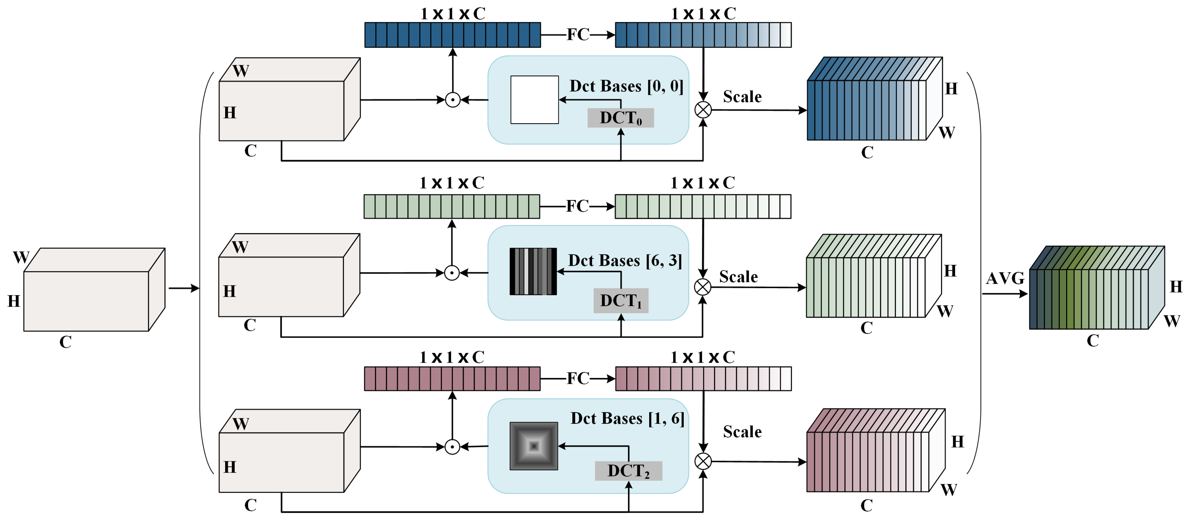
We propose a multi-branch channel attention structure to fulfill MbsCANet, in which three kinds of frequency components are mined to compress and represent channels.

(3)

In comparison to existing well-known spectral-based channel attention techniques (SENet and FcaNet), our model performs well and also achieves competitive or better results against state-of-the-art methods on the breast cancer histopathology image dataset.

The remainder of this paper is structured as follows: Section 2 describes the given method, which includes the related background of DCT and spectral channel attention. Experiments and comparisons are conducted in Section 3. The conclusions are presented in Section 4.

2. Methodology

In this section, we first briefly review the formulation of DCT, and the related spectral-channel-attention-based SENet and FcaNet are reviewed in Section 2.1 and Section 2.2. Then, we extend SENet and FcaNet and propose a multi-branch spectral channel attention network, i.e., the MbsCANet, in Section 2.3.

2.1. Discrete Cosine Transform (DCT)

The compression of channels should be of a high data compression ratio with high quality. In signal processing, e.g., digital images and videos, discrete cosine transform (DCT), similar to the discrete Fourier transform, is a widely used data compression technology to compress JPEG, HEIF, MPEG, and H.26x. It can transform a signal or image from the spatial domain to the frequency domain. As DCT possesses the good properties of compaction and being differentiable, it naturally becomes a suitable choice for channel attention to compress a channel to only a scalar that can be integrated into CNNs for end-to-end learning.

The DCT [23,25] represents an image as a sum of the cosines of varying magnitudes and frequencies. For a typical image, most of the visually significant information about the image is concentrated in just a few coefficients of the DCT. The basis function of 2D DCT can be written as:

$$\begin{array}{cc}\hfill & B_{h,w}^{i,j}=cos(\frac{\pi h}{H}(i+\frac{1}{2}))cos(\frac{\pi w}{W}(j+\frac{1}{2}))\hfill \\ \hfill & \mathrm{s}.\mathrm{t}.h\in \{0,1,\dots ,H-1\},w\in \{0,1,\dots ,W-1\}\hfill \end{array}$$

(1)

where H and W are the height and width of the two-dimensional image. Therefore, $B_{h,w}^{i,j}$ is a fixed value. For a given two-dimensional feature map X with a spatial size of $H\times W$, its 2D DCT can be defined by multiplying and summing X and $B_{h,w}^{i,j}$, which is defined as:

$$\begin{array}{cc}\hfill & F_{h,w}=\sum _{i=0}^{H-1}\sum _{j=0}^{W-1}{X}_{i,j}{B}_{h,w}^{i,j}\hfill \\ \hfill & \mathrm{s}.\mathrm{t}.h\in \{0,1,\dots ,H-1\},w\in \{0,1,\dots ,W-1\}\hfill \end{array}$$

(2)

where $F_{h,w}$ with the same spatial size of $H\times W$ is the frequency spectrum of 2D DCT, also called the DCT coefficients of X. The DCT is an invertible transform; we can obtain the expression of 2D DCT of X according to Equation (2) as follows:

$$\begin{array}{cc}\hfill & X_{h,w}=\sum _{h=0}^{H-1}\sum _{w=0}^{W-1}{F}_{h,w}{B}_{h,w}^{i,j}\hfill \\ \hfill & \mathrm{s}.\mathrm{t}.i\in \{0,1,\dots ,H-1\},j\in \{0,1,\dots ,W-1\}\hfill \end{array}$$

(3)

Intuitively, via the inverse DCT, any input of size $H\times W$ can be written as a sum of $HW$ basis functions. The DCT coefficients $F_{h,w}$ can be regarded as the weights applied to each basis function. For simplicity, some constant normalizations are removed in Equations (2) and (3).

In Equation (2), 2D DCT can be viewed as a weighted sum of inputs. Typically, global average pooling (GAP) is a commonly used, simple but effective compression method along the channel dimension in channel attention. Through the formulations above, when both h and w are 0, we have:

$$\begin{array}{cc}\hfill F_{0,0}& =\sum _{i=0}^{H-1}\sum _{j=0}^{W-1}{X}_{i,j}cos\left(\frac{0}{H}\left(i+\frac{1}{2}\right)\right)cos\left(\frac{0}{W}\left(j+\frac{1}{2}\right)\right)\hfill \\ & =\sum _{i=0}^{H-1}\sum _{j=0}^{W-1}{X}_{i,j}\hfill \\ & =HW\times GAP\left(X\right)\hfill \end{array}$$

(4)

For a certain feature map, $HW$ is a fixed constant. It is not difficult to see from Formula (4) that the lowest frequency component $F_{0,0}$ in 2D DCT is proportional to the GAP in SENet. Thus, we can say that GAP is actually a special case contained in 2D DCT.

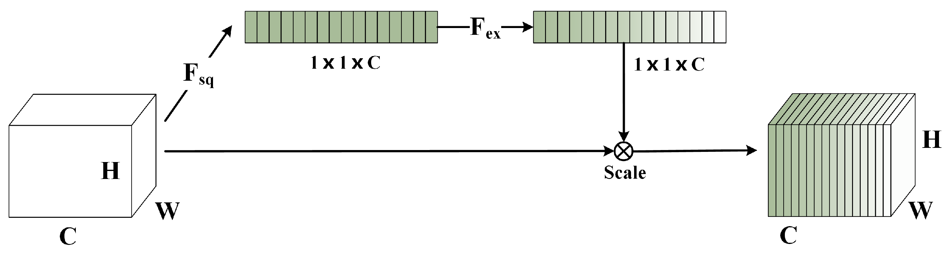
2.2. Spectral-Channel-Attention-Based SENet and FcaNet

In the context of CNNs, channel attention [7,8,9,23,26,27,28] is widely used for various tasks and the basic principle is to use a scalar to represent and evaluate the importance of each channel. Since a single, whole channel is represented using a scalar only, the necessary compression method is needed to compress the input feature map X with the size of $C\times H\times W$ into a C-dimensional vector to represent C channels in X. After the compression (or squeeze) operation, the attention map (attm) is formulated by

$$\begin{array}{c}\hfill attm=sigmoid\left(fc\left(compression\left(X\right)\right)\right)\end{array}$$

(5)

where $fc$ are two fully connected layers for mapping. The $sigmoid$ function is for transforming entries in $attm\in {\mathbb{R}}^C$ to numbers between 0 and 1, and each entry refers to the importance of the corresponding channel.

Then, each channel of the input X is scaled by the corresponding attention value to produce the attentive channel. It is achieved by

$$\begin{array}{c}\hfill {\tilde{X}}_i=att{m}_i{X}_i,s.t.i\in \{0,1,\dots ,C-1\}\end{array}$$

(6)

where $att{m}_i$ and $X_i$ denote the i-th entry in $attm$ and i-th channel in X, respectively. $\tilde{X}$ is the final attentive output of channel attention with same size of input X, which enables such a channel attention module to be inserted into any layer in CNN models.

SENet [7] and FcaNet [23] are two well-known spectral-channel-attention-based networks which are closely related to ours. SENet is formulated as the squeeze ($F_{sq}$) and excitation ($F_{sq}$) operations shown in Figure 3. The squeeze in SENet, generating global description, is achieved by GAP; i.e., the compression function in Equation (5) is equal to GAP. The excitation shares the similar calculation process in Equations (5) and (6). As proved above, GAP is the component of the lowest frequency in 2D DCT. Naturally, SENet explores the spectral correlation in channel attention. Going beyond SENet and following the same design philosophy, FcaNet uniformly groups all channels, and channels in the same group are compressed by the same frequency component of 2D DCT, and the channels in other groups are compressed by different frequency components. Thus, FcaNet is a multi-spectral channel attention network. Based on these works, a new channel attention network, the MbsCANet, is proposed, incorporating frequency components into the multi-branch structure described next.

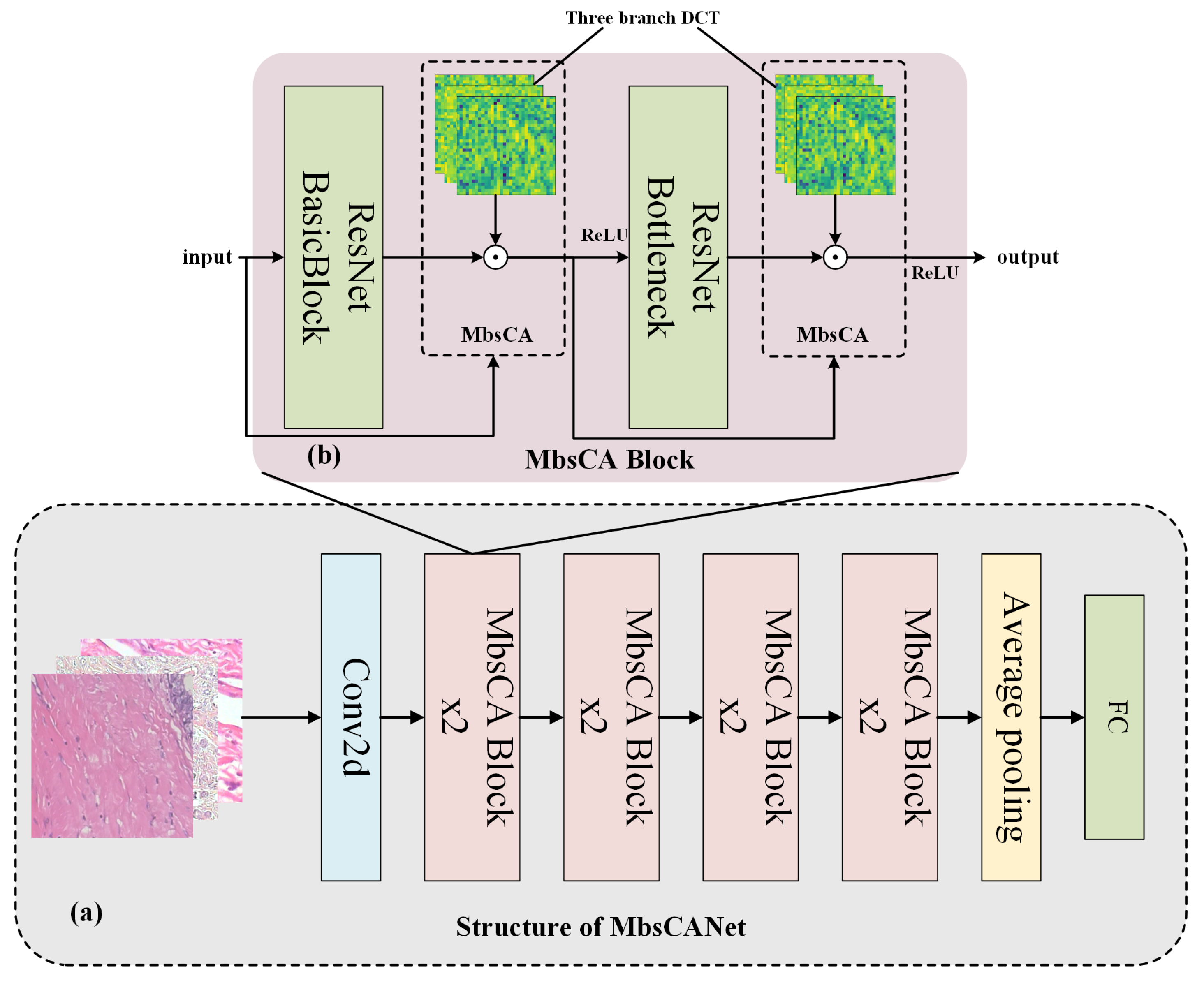
2.3. Multi-Branch Spectral Channel Attention Network (MbsCANet)

In this section, we first present the general structure of the proposed MbsCANet for the histopathological image classification task for breast cancer. Then, the core module of the multi-branch spectral channel attention (MbsCA) in the MbsCANet is illustrated in detail.

2.3.1. General Structure

The overall structure of the MbsCANet is shown in Figure 1a, and its key component MbsCANet module is illustrated in Figure 1b, in which a multi-branch structure of the MbsCA is displayed in Figure 2. We utilize ResNet18 as the basic network to form our MbsCANet, which can be efficiently trained for fast inference. Each MbsCANet module in the MbsCANet consists of a basic block in ResNet18 and an MbsCA. The MbsCA is inserted into the end of a basic block and does not change its topological structure. Such a design enables us to reuse the weights of ResNet18, avoiding training a network from scratch that is prohibitive due to insufficient breast cancer histopathological images. The network is more inclined to the interaction with high- and low-frequency information. Using the channel attention mechanism, the network can learn more meaningful information and reduce the influence of worthless information. Because the main information of one image is concentrated in the low-frequency region [7,20,22,23] and the texture image has a complex distribution of high and low frequencies, we thus propose to use a multi-branch network to selectively interact with the part of the low-frequency information with the channel features of the input images. Our model can be trained end-to-end while slightly increasing a few parameters and takes into account the advantages of the characteristics of the frequency information and the rich context of simple operations. Notably, our MbsCANet structure is very flexible and interchangeable. It is a plug-and-play attention module. Our attention module can be inserted anywhere in the basic CNN network by simply setting the number of output channels. The number of output channels is the same as the number of output channels of the previous layer instead of being instantiated in ResNet18 and applied to other medical image classification tasks.

2.3.2. Multi-Branch Spectral Channel Attention Module

SENet actually exploits only the lowest frequency information, while the information of other frequencies is discarded completely. Although FcaNet explores the multiple frequency components of 2D DCT, the individual frequency component is merely used to represent part of channels in a feature map. Each single channel represented by multiple frequency components is more reasonable and deserves further exploration, but that is not modeled in FcaNet at all. Therefore, the multi-branch spectral channel attention module is proposed to solve this limitation.

Figure 2 gives an overview of the multi-branch spectral channel attention module (MbsCA). In the MbsCA, each branch attention focuses on highlighting important features of the input from a different frequency perspective. More generally, such a branch can be a channel attention, spatial attention, and other dimensions to achieve cross-latitude interactive computation. Here, our purpose is to achieve spectral channel attention following the similar computation process in SENet. Each branch employs an individual frequency component and any two branches capture different frequency components. In accomplishing this, multiple frequency components are explored, solving the problem of the incomplete utilization of the frequency information in the image, and the interaction between multiple frequency components is realized through the multi-branch structure.

As shown in Figure 2, the MbsCA redesigns the input stream and weight structure. The input $X\in {\mathbb{R}}^{H\times W\times C}$ is first copied K times to obtain K identical X, denoted as $\{X_0,\dots ,X_{K-1}\}$. In each branch, we assign a corresponding frequency component of 2D DCT. First, the 2D DCT for the input $X_k$ is expressed as

$$\begin{array}{cc}\hfill & Fre{q}_k=2DDC{T}_{{\mathrm{\Omega }}_k}\left(X_k\right)=\sum _{h=0}^{H-1}\sum _{w=0}^{W-1}{X}_k{B}_{h,w}^{{\mathrm{\Omega }}_k}\hfill \\ \hfill & s.t.k\in \{0,1,\dots ,K-1\}\hfill \end{array}$$

(7)

where $Fre{q}_k\in {\mathbb{R}}^C$ is the spectral vector in the k-th branch, i.e., $Fre{q}_k=compression\left(X_k\right)$ in Equation (5). The $2DDCT$ represents the frequency component of the 2D DCT corresponding to $X_k$. ${\mathrm{\Omega }}_k$ is the frequency component 2D indices.

Then, $Fre{q}_k$ is used to predict the weights of all channels in $X_k$ and scale them subsequently. It goes through $FC$ layers for adaption, and a $sigmoid$ function is adopted to map entries to the range of 0 to 1. The scaled new features ${\overline{X}}_k$ in this single branch are obtained by

$$\begin{array}{cc}\hfill & att{m}_k=sigmoid\left(fc\left(Fre{q}_k\right)\right)\hfill \end{array}$$

(8)

$$\begin{array}{cc}\hfill & {\overline{X}}_k=att{m}_k{X}_k\hfill \end{array}$$

(9)

Equations (8) and (9) are responsible for predicting weights $att{m}_k$ and scaling input $X_k$, respectively.

For all K branches in the MbsCA, we repeat Equations (7)–(9) above, obtaining channel attentive features $\{{\overline{X}}_0,\dots ,{\overline{X}}_{K-1}\}$. The attentive features obtained on the all branches are averaged as the final output of our MbsCA module, which is computed as

$$\begin{array}{cc}\hfill & Y=AVG\left(\left\{{\overline{X}}_0,{\overline{X}}_1,\dots ,{\overline{X}}_{K-1}\right\}\right)\hfill \end{array}$$

(10)

where $AVG$ is an average pooling to fuse $X_k$, allowing different frequency components on each single channel to interact. The output Y has the same shape with input X, enabling our MbsCA to be flexibly plugged into any layers of the basic network without changing its topology that can share its pretrained weights. Regarding the selection of the frequency components on the K branches ($K=3$ in our experiments), we conduct ablation experiments to evaluate the importance of several frequency components individually and then select Top-K frequency components with the highest performance based on the results.

In contrast, although FcaNet also introduces different frequency components to enrich features, only one frequency component is used in each part of the channel features. It fails to represent a single channel via different frequency components and thus ignores the interaction between frequency components, resulting in insufficient channel modeling. As for SENet, it does not make use of multiple frequency components at all and is a special case of ours. Among them, our MbsCANet exhibits better experimental results (see Section 3).

3. Experiments

In this section, we first elaborate on the relevant details of our experiments in Section 3.1. Next, ablation experiments are carried out to demonstrate the effectiveness of the proposed MbsCANet in Section 3.2. Then, comparisons with state-of-the-art methods are given in Section 3.3. Finally, visualization results and corresponding analysis are provided in Section 3.4.

3.1. Implementation Details

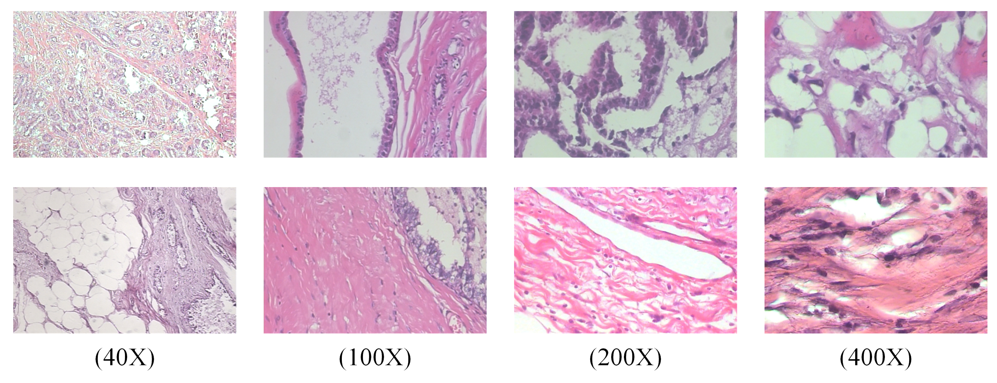
3.1.1. Dataset

We utilize the BreakHis dataset to evaluate the proposed MbsCANet. It is one of the first (2016) publicly available large-scale non-full-field breast cancer histopathology image datasets (online at http://www.inf.ufpr.br/vri/databases/BreaKHis_v1.tar.gz (accessed on 15 October 2020)) and provides a good benchmark for this medical application. A total of 7909 medical imaging samples are contained, including 2480 benign tumors (fibroadenoma, adenoma, tubular adenoma, and trichomes tumors) and 5429 malignant tumors (lobular carcinoma, ductal carcinoma, papillary carcinoma, and mucinous carcinoma). Each sample image is 700 × 460 pixels in size and is displayed directly on the pathological area of the breast tumor in RGB color. Each sample is divided into four different magnification factors: 40×, 100×, 200×, and 400×. Figure 4 shows a typical sample of breast cancer histopathology images from the BreakHis dataset at different magnifications.

3.1.2. Evaluation Metrics and Setting

In this work, the commonly used metrics of the image-level recognition rate and patient-level recognition rate are adopted to evaluate our method. In addition to both, according to the recommendations of the study on processing binary balanced data [29], the following performance criteria are also provided to measure the image-level diagnostic performance of the benign and malignant categories: Accuracy, Precision, Recall, and F1-Score.

For the hyperparameters of network training, the initial learning rate is set to 0.001, and the decay of the learning rate reduces to half of the current learning rate for every five iterations. We use random shuffling for the dataset to prevent the chance of learning from the ordered training set data. The SGD optimizer with momentum set to 0.9 is employed, which prevents the loss function from falling into a local optimum solution and thus controls the loss function to a global minimum. All models are trained with cosine learning rate decay and label smoothing within 100 epochs. All experiments are performed on a server equipped with an NVIDIA RTX 3090 GPU using the Pytorch [30] deep learning framework.

3.2. Ablation Study

In this section, we first provide an ablation study on the individual frequency components in image-level recognition in Section 3.2.1. Other metrics of the MbsCANet under Accuracy, Precision, Recall, and F1-Score are given in Section 3.2.2. We make comparisons with our key counterparts in Section 3.2.3.

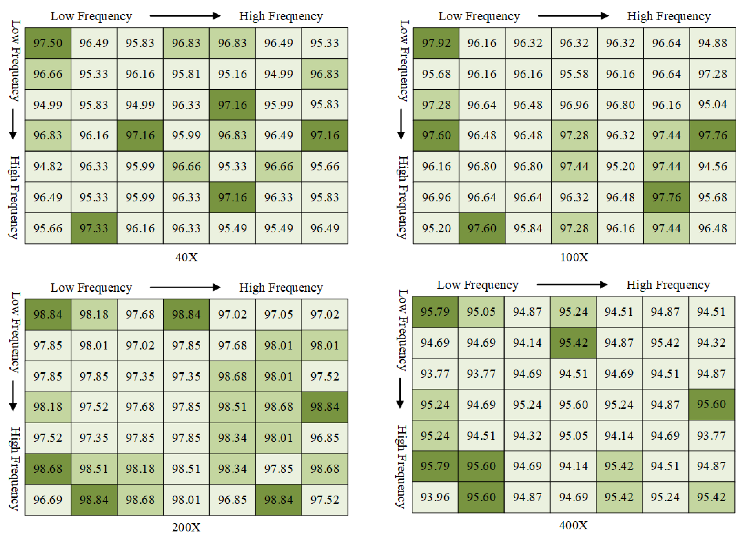
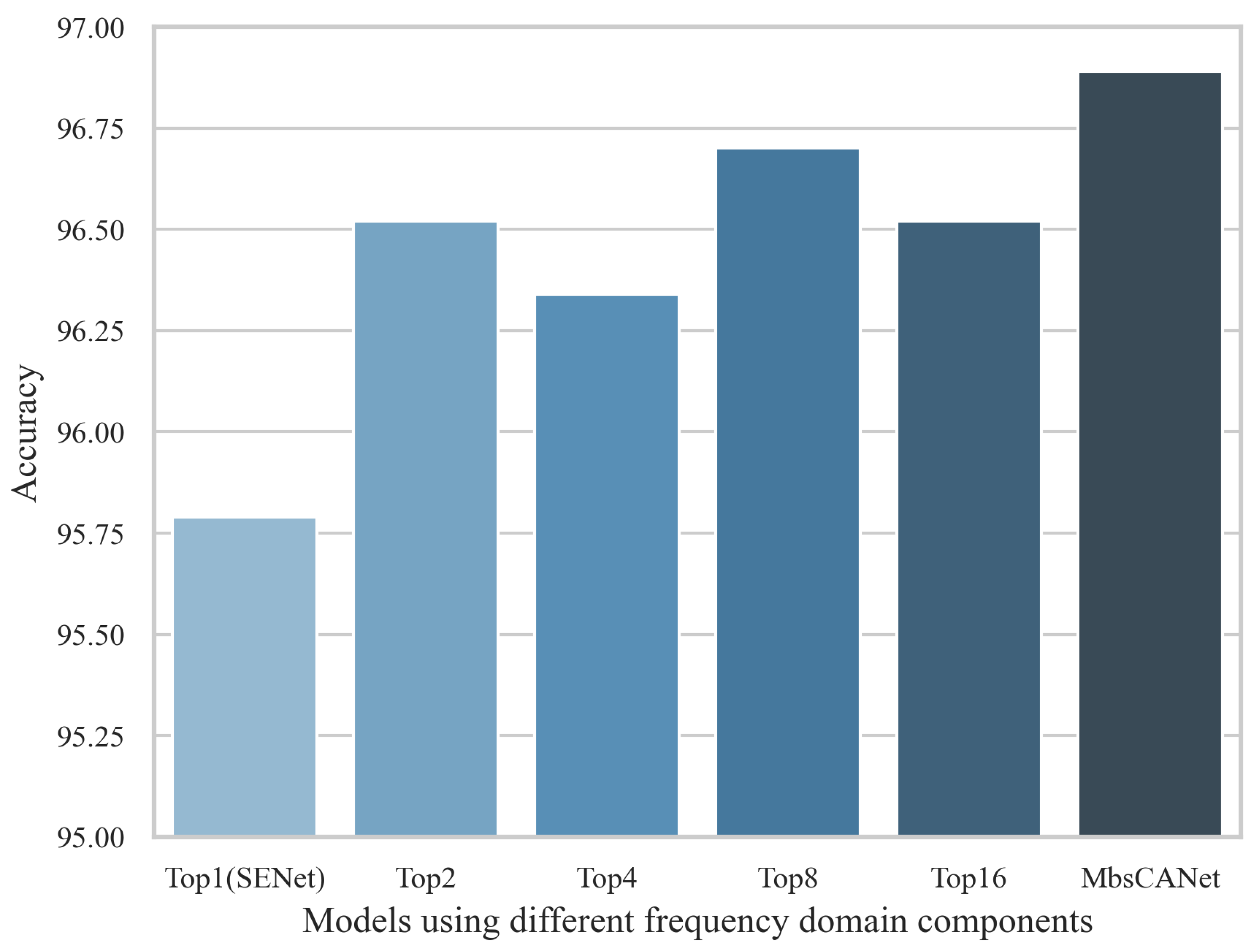
3.2.1. Ablation on Individual Frequency Components

In our MbsCANet, we need to select the appropriate frequency components on breast cancer pathology images. Here, ablation experiments on these are performed on the BreakHis dataset to select K (=3) such frequency components.

The basic network of ResNet18 used to instantiate our MbsCANet is pretrained on ImageNet, where its last feature map is of spatial size of $7\times 7$. Following FcaNet [23], there are 49 experiments to individually evaluate one single frequency component, because for a $7\times 7$ matrix, it has 49 basis functions, meaning that the whole 2D DCT frequency space is divided into $7\times 7$ parts. As samples in the BreakHis dataset have four different magnification factors, each such ablation experiment is conducted on four subdatasets of the BreakHis dataset. Figure 5 illustrates the corresponding accuracies. In all four subdatasets, the lowest frequency component (i.e., GAP in SENet) is the optimal component. It can be concluded that the neural network is more inclined to low-frequency information, which is consistent with previous works [7,20,22,23]. Further, other frequency components also encode useful information to represent the channels, which cannot be ignored completely. And the high-frequency component in the image spectrum is closely related to texture, so a single channel compressed by different frequency components is more reasonable and helpful for boosting performance. Based on the experimental results in Figure 5, we first sort the components according to their importance in each subdataset. Then, the K frequency components that perform well on the four subdatasets are selected to form the final branch structure.

In order to verify that our three-branch multi-spectral combination is optimal for breast cancer pathology images, we offer comparison results for different combinations of quantitative components at 400× magnification, as shown in Figure 6. Among them, Top-{2,4,8,16} are the combination of the relevant number of components used in FcaNet. Top-1 in the horizontal axis refers to SENet, where only the lowest frequency component is explored to compress channels. For the case of FcaNet, we try our best to tune it with the official code for achieving better image-level performance. As the default setting, Top-16 in FcaNet gains the best performance in ImageNet classification, while in terms of breast cancer pathology image classification, this setting may not be the best one. Instead of using the default setting of Top-16, after our careful evaluation, Top-8 in FcaNet is the best setting (96.7%). In contrast to FcaNet, our three-branch structure MbsCANet (marked with an orange star) represents each single channel with three components instead of one in both FcaNet and SENet and achieves better results. As the main counterparts of our MbsCANet, we will make individual comparisons with both in the next section.

3.2.2. Accuracy, Precision, Recall, and F1-Score Results

In order to further verify the robustness and generalization ability of the MbsCANet, four other typical evaluation metrics (i.e., Accuracy, Precision, Recall, and F1-Score) are utilized to evaluate it. The results are listed in

Table 1. Precision, Recall, F1-Score, and Accuracy results (%) achieved by MbsCANet on BreakHis dataset.

Magnification	Accuray	Precision	Recall	F1-Score
40×	97.66	97.79	94.65	96.19
100×	97.92	97.35	95.83	96.58
200×	99.01	99.40	97.08	98.22
400×	96.89	95.24	94.67	94.95

.

From Table 1, all four metrics of the MbsCANet are higher than 97% for the 200× dataset, and Accuracy and Precision results even exceed 99%. What is more is that the results under any metrics achieved by any magnification factors in the BreakHis dataset reach over 94%, each of which is a high score. These satisfied performance under the four metrics and can verify the powerful robustness and generalization capability of the MbsCANet from different views.

3.2.3. Comparisons with Counterparts

As FcaNet and SENet are two main counterparts, we compare both in terms of image-level recognition and patient-level recognition, respectively. Additionally, a baseline method is also provided as a reference that the vanilla ResNet18 is directly used in recognition without any channel attention. The comparison results for the four magnification factors of the BreakHis dataset are shown in

Table 2. Experimental results (%) of each model at the image level.

Method	40×	100×	200×	400×
Baseline	96.16	95.84	97.35	93.77
SENet	97.50	97.92	98.84	95.79
FcaNet	97.49	97.12	98.18	96.70
MbsCANet	97.66	97.92	99.01	96.89

and

Table 3. Experimental results (%) for each network at the patient level.

Method	40×	100×	200×	400×
Baseline	95.99	96.29	97.59	94.33
SENet	96.82	96.03	98.19	96.69
FcaNet	96.76	97.47	98.46	96.17
MbsCANet	97.17	97.98	98.87	97.06

, respectively.

Table 2 reports image-level recognition. From it, we can see that the MbsCANet achieves recognition rates of 97.49%, 97.12%, 98.18%, and 96.52% on 40×, 100×, 200× and 400× magnification, respectively. FcaNet is a multi-spectral channel attention model as well, where each grouped channel is compressed of a frequency component of 2D DCT, and channels from different groups are compressed by different frequency components. Essentially, one single channel is compressed by a single frequency component. By contrast, our MbsCANet represents a single channel with three components and outperforms FcaNet in terms of all magnification factors. As a special spectral channel attention model, SENet only focuses on the lowest frequency component, i.e., GAP. Unexpectedly, its performance is lower than both FcaNet and MbsCANet. The baseline model, i.e., vanilla ResNet18, draws the worst results. All three spectral channel attention models significantly surpass it by a large margin. These comparisons conclude that spectral channel attention is effective and can improve basic networks, and our multi-branch structure design of the MbsCANet to explore multiple frequency components is more reasonable and reports the best results.

Similarly, at the patient-level recognition shown in Table 3, our MbsCANet obtains 97.17%, 97.98%, 98.87%, and 97.06% recognition rates on the four subdatasets, respectively. Compared with the baseline, performance improvements are 1.18%, 1.69%, 1.28%, and 2.73% in Accuracy. In contrast to FcaNet and SENet, MbsCANet yields average improvements of 0.41% and 0.84%, respectively. These comparisons consistently prove the conclusion above again and meet our claim.

3.3. Comparisons with State-of-the-Art Methods

To demonstrate the advanced performance of the MbsCANet for breast cancer pathology image classification, we further compare it with several representative CNN-based methods from the past five years. The comparison results are shown in Table 4.

In Table 4, all comparisons are also from image-level recognition and patient-level recognition on four magnification factors in the BreakHis dataset. Among comparison methods, Zhou et al. [31] report better performance at image-level recognition with 94.43%, 98.31%, 99.14%, and 93.35% on 40×, 200×, 200× and 400× magnification. However, it exploits the complicated multi-scale dense network as the backbone, while ours only employs the lightweight ResNet18 as the backbone. Even so, our MbsCANet still exceeds it, especially for the 400× magnification, for which the gain is 3.54%. For patient-level recognition, Zhou et al. [31] also show good results of 96.16%, 97.91%, 98.83%, and 92.64% for the four magnification factors. Similarly, MbsCANet is superior to it as well and the gain is over 4% for the 400× magnification. Additionally, in contrast to other previous methods, the improvements are much larger in terms of both image-level recognition and patient-level recognition. The extensive comparisons in Table 4 demonstrate the superiority of our MbsCANet and show great potential for employing frequency characteristics in deep models for breast cancer pathological image classification scenarios.

AMin et al.’s [32] paper achieved good results at 40× magnification, but MbsCANet outperformed their method at other magnifications, especially at 100× magnification, where the image-level and patient-level gains were 8.28% and 8.72%, respectively. Overall, the MbsCANet outperforms their method.

At the same time, in order to show that the MbsCANet model has good results in breast cancer pathology image classification tasks, we also conducted experiments on the BACH dataset (ICIAR2018_BACH_Challenge) and compared it with the basic model. From the experimental results, we can see that the MbsCANet model has a good effect on breast cancer pathology. Image classification accuracy has been significantly improved. Table 5 shows the experimental results.

Table 4. Comparisons of image-level and patient-level recognition rates (%) on the BreakHis dataset with representative CNN-based approaches.

Reference	Year	Method	Images Level				Patient Level
			40×	100×	200×	400×	40×	100×	200×	400×
Benhammou et al. [33]	2018	InceptionV3	90.20	85.60	86.10	82.50	91.50	85.10	86.80	82.90
Alom et al. [34]	2019	IRRCNN	97.16	96.84	96.61	95.78	96.69	96.37	96.27	96.37
Sudharshan et al. [35]	2019	PFTAS + NPMIL	87.8 ± 5.6	85.6 ± 4.3	80.8 ± 2.8	82.9 ± 4.1	92.1 ± 5.9	89.1 ± 5.2	87.2 ± 4.3	82.7 ± 4.0
Lichtblau et al. [36]	2019	DE ensemble	85.60	87.40	89.80	87.00	83.90	86.00	89.10	86.60
Zhang et al. [37]	2020	VGG-VD16	95.03	90.41	88.48	85.00	95.50	91.57	89.20	89.20
Hou [38]	2020	22 layers CNN	90.89	90.99	91.00	90.97	91.00	91.00	91.00	91.00
Man et al. [39]	2020	DenseNet121-AnoGAN	99.13 ± 0.2	96.39 ± 0.7	86.38 ± 1.2	85.20 ± 2.1	96.32 ± 1.3	95.89 ± 0.9	86.91 ± 2.0	85.16 ± 1.3
Gour et al. [40]	2020	IDSNet	87.4 ± 3.0	87.2 ± 3.5	91.1 ± 2.3	86.2 ± 2.1	87.4 ± 3.3	88.1 ± 2.9	92.5 ± 2.8	87.7 ± 2.4
Togacar et al. [41]	2020	BreastNet	97.99	97.84	98.51	95.88	n/a	n/a	n/a	n/a
Wang et al. [42]	2021	FE-BkCapsNet	92.71 ± 0.16	94.52 ± 0.11	94.03 ± 0.25	93.54 ± 0.24	n/a	n/a	n/a	n/a
Ibraheem et al. [43]	2021	3PC NNB-N et	92.27	93.07	97.04	92.09	n/a	n/a	n/a	n/a
Li et al. [44]	2021	Sliding + Class Balance Random	87.85 ± 2.69	86.68 ± 2.28	87.75 ± 2.37	85.30 ± 4.41	87.93 ± 3.91	87.41 ± 3.26	88.76 ± 2.50	85.55 ± 4.03
Hao et al. [45]	2021	APVEC	92.10	90.20	95.00	92.80	n/a	n/a	n/a	n/a
Zhou et al. [31]	2022	RANet+ADSVM	94.43 ± 0.8	98.31 ± 0.3	99.14 ± 0.2	93.35 ± 0.9	96.16 ± 0.9	97.91 ± 0.4	98.83 ± 0.3	92.64 ± 0.9
Chattopadhyay et al. [46]	2022	DRDA-Net7	95.72	94.41	97.43	96.84	n/a	n/a	n/a	n/a
Djouima et al. [47]	2022	DCGAN	96.00	95.00	88.00	92.00	n/a	n/a	n/a	n/a
AMin et al. [32]	2023	FabNet	99.03	89.68	98.51	97.10	99.01	89.26	98.38	96.96
MbsCANet (ours)	-	Mutiple Spectral Channel Attention	97.66	97.92	99.01	96.89	97.17	97.98	98.87	97.06

n/a means that results are unavailable.

Table 4. Comparisons of image-level and patient-level recognition rates (%) on the BreakHis dataset with representative CNN-based approaches.

Reference	Year	Method	Images Level				Patient Level
			40×	100×	200×	400×	40×	100×	200×	400×
Benhammou et al. [33]	2018	InceptionV3	90.20	85.60	86.10	82.50	91.50	85.10	86.80	82.90
Alom et al. [34]	2019	IRRCNN	97.16	96.84	96.61	95.78	96.69	96.37	96.27	96.37
Sudharshan et al. [35]	2019	PFTAS + NPMIL	87.8 ± 5.6	85.6 ± 4.3	80.8 ± 2.8	82.9 ± 4.1	92.1 ± 5.9	89.1 ± 5.2	87.2 ± 4.3	82.7 ± 4.0
Lichtblau et al. [36]	2019	DE ensemble	85.60	87.40	89.80	87.00	83.90	86.00	89.10	86.60
Zhang et al. [37]	2020	VGG-VD16	95.03	90.41	88.48	85.00	95.50	91.57	89.20	89.20
Hou [38]	2020	22 layers CNN	90.89	90.99	91.00	90.97	91.00	91.00	91.00	91.00
Man et al. [39]	2020	DenseNet121-AnoGAN	99.13 ± 0.2	96.39 ± 0.7	86.38 ± 1.2	85.20 ± 2.1	96.32 ± 1.3	95.89 ± 0.9	86.91 ± 2.0	85.16 ± 1.3
Gour et al. [40]	2020	IDSNet	87.4 ± 3.0	87.2 ± 3.5	91.1 ± 2.3	86.2 ± 2.1	87.4 ± 3.3	88.1 ± 2.9	92.5 ± 2.8	87.7 ± 2.4
Togacar et al. [41]	2020	BreastNet	97.99	97.84	98.51	95.88	n/a	n/a	n/a	n/a
Wang et al. [42]	2021	FE-BkCapsNet	92.71 ± 0.16	94.52 ± 0.11	94.03 ± 0.25	93.54 ± 0.24	n/a	n/a	n/a	n/a
Ibraheem et al. [43]	2021	3PC NNB-N et	92.27	93.07	97.04	92.09	n/a	n/a	n/a	n/a
Li et al. [44]	2021	Sliding + Class Balance Random	87.85 ± 2.69	86.68 ± 2.28	87.75 ± 2.37	85.30 ± 4.41	87.93 ± 3.91	87.41 ± 3.26	88.76 ± 2.50	85.55 ± 4.03
Hao et al. [45]	2021	APVEC	92.10	90.20	95.00	92.80	n/a	n/a	n/a	n/a
Zhou et al. [31]	2022	RANet+ADSVM	94.43 ± 0.8	98.31 ± 0.3	99.14 ± 0.2	93.35 ± 0.9	96.16 ± 0.9	97.91 ± 0.4	98.83 ± 0.3	92.64 ± 0.9
Chattopadhyay et al. [46]	2022	DRDA-Net7	95.72	94.41	97.43	96.84	n/a	n/a	n/a	n/a
Djouima et al. [47]	2022	DCGAN	96.00	95.00	88.00	92.00	n/a	n/a	n/a	n/a
AMin et al. [32]	2023	FabNet	99.03	89.68	98.51	97.10	99.01	89.26	98.38	96.96
MbsCANet (ours)	-	Mutiple Spectral Channel Attention	97.66	97.92	99.01	96.89	97.17	97.98	98.87	97.06

n/a means that results are unavailable.

Table 5. Experimental results on BACH dataset.

Method	Accuracy
Baseline	75%
MbsCANet	86%

Table 5. Experimental results on BACH dataset.

Method	Accuracy
Baseline	75%
MbsCANet	86%

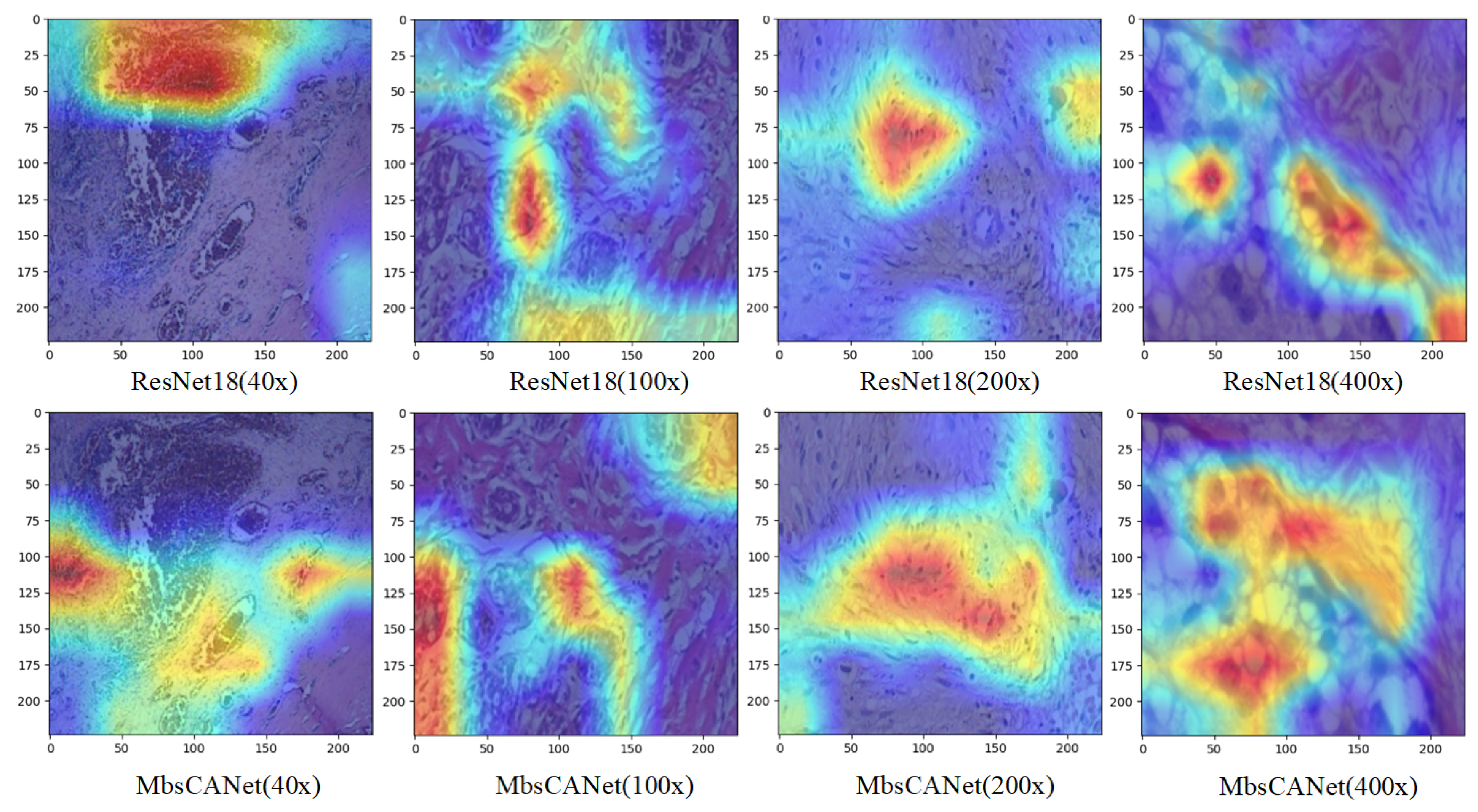
3.4. Visualization Results

We give visualization results to further demonstrate the effect of our network, as shown in Figure 7. In Figure 7, we randomly choose images with four magnification factors in the BreakHis dataset that are misclassified by the backbone network ResNet18 but can be correctly classified by the proposed MbsCANet. Heat maps visualize the areas of interest for different networks for a given category in the same image. By analyzing the feature details in this section, we discuss the reasons for the misclassification of the backbone model.

It can be seen that from the breast cancer pathology images, the texture of breast cancer pathology tissue sections is more complex. Therefore, the backbone network is affected in feature extraction when images have insufficient features and there is a bias in the region of interest of the features, leading to misclassification. Differently, the proposed network takes advantage of the information of the multiple frequency components for the features and achieves interaction between them simultaneously. Its feature extraction and modeling capability are significantly enhanced to focus on the key feature regions that are not highlighted by the backbone network. Thus, our model has stronger classification ability than the vanilla backbone and the other simple channel attention models of SENet and FcaNet.

We also randomly choose a pathological image of breast cancer, and the DCT spectrum distribution at 40×, 100×, 200×, and 400× magnification is shown in Figure 8. These graphs visualize the frequency components of the images, where the ‘Z’ axis represents the amplitude of the DCT coefficients, and the ‘H’ and ‘W’ axes correspond to the two-dimensional spatial frequency components. It can be seen that in the pathological images of breast cancer, although the models are mainly concentrated in the low-frequency region, the high-frequency region still contains some characteristic information. Among the four magnification factors, 40×, 100×, and 200× images contain more information in the high-frequency region than the 400× images. To this end, the reasonable use of both low- and high-frequency components is necessary and should be considered deeply and in line with practical applications. This analysis also demonstrates the underlying reason why the MbsCANet attains better results using multiple frequency components for breast cancer pathological image classification.

4. Conclusions

In this paper, we emphasize the importance of frequency domain analysis in breast cancer histopathology image classification, introducing our advanced MbsCANet model. This model innovatively processes different frequency components of 2D DCT in a multi-branch framework, enabling a more nuanced understanding of the frequency characteristics inherent in histopathology images. The multi-branch approach allows the MbsCANet to effectively capture and integrate a wide range of frequency information, from low-frequency components that represent the general patterns and shapes in the images to high-frequency components that capture finer details and textures. This comprehensive frequency analysis ensures a robust and detailed interpretation of histopathology images, contributing to the model’s high accuracy in classification. The MbsCANet model is more suitable for images with high image contrast and clear edges. Low-resolution images with blurred edges are not well recognized. Our results for the BreaKHis dataset, with image- and patient-level recognition accuracies of 97.87% and 97.77%, respectively, demonstrate the potential of frequency domain analysis in enhancing the accuracy and efficiency of medical image classification, paving the way for its application in clinical settings for rapid and precise cancer diagnosis.

In future work, we plan to further optimize the MbsCANet by combining feature distribution and frequency components and introducing a spatial attention mechanism to improve model performance. In addition, we will explore the potential of MbsCANet in other medical image application fields and expand its application scope in the field of medical imaging and diagnosis. This will not only test the versatility of MbsCANet but also make an important contribution to the field of medical image analysis.

References

1. Ferlay, J.; Colombet, M.; Soerjomataram, I.; Parkin, D.M.; Piñeros, M.; Znaor, A.; Bray, F. Cancer statistics for the year 2020: An overview. Int. J. Cancer 2021, 149, 778–789. [Google Scholar] [CrossRef] [PubMed]
2. Xue, Y.; Ye, J.; Zhou, Q.; Long, L.R.; Antani, S.; Xue, Z.; Cornwell, C.; Zaino, R.; Cheng, K.C.; Huang, X. Selective synthetic augmentation with HistoGAN for improved histopathology image classification. Med. Image Anal. 2021, 67, 101816. [Google Scholar] [CrossRef] [PubMed]
3. Dif, N.; Attaoui, M.O.; Elberrichi, Z.; Lebbah, M.; Azzag, H. Transfer learning from synthetic labels for histopathological images classification. Appl. Intell. 2022, 52, 358–377. [Google Scholar] [CrossRef]
4. Burçak, K.C.; Baykan, Ö.K.; Uğuz, H. A new deep convolutional neural network model for classifying breast cancer histopathological images and the hyperparameter optimisation of the proposed model. J. Supercomput. 2021, 77, 973–989. [Google Scholar] [CrossRef]
5. Deng, J.; Dong, W.; Socher, R.; Li, L.; Li, K.; Li, F. Imagenet: A large-scale hierarchical image database. In Proceedings of the 2009 IEEE Conference on Computer Vision and Pattern Recognition, Los Alamitos, CA, USA, 20–25 June 2009; pp. 248–255. [Google Scholar]
6. Russakovsky, O.; Deng, J.; Su, H.; Krause, J.; Satheesh, S.; Ma, S.; Huang, Z.; Karpathy, A.; Khosla, A.; Bernstein, M. Imagenet large scale visual recognition challenge. Int. J. Comput. Vis. 2015, 115, 211–252. [Google Scholar] [CrossRef]
7. Hu, J.; Shen, L.; Sun, G. Squeeze-and-excitation networks. In Proceedings of the IEEE Conference on Computer Vision and Pattern Recognition, Salt Lake City, UT, USA, 18–22 June 2018; pp. 7132–7141. [Google Scholar]
8. Woo, S.; Park, J.; Lee, J.Y.; Kweon, I.S. Cbam: Convolutional block attention module. In Proceedings of the European Conference on Computer Vision (ECCV), Munich, Germany, 8–14 September 2018; pp. 3–19. [Google Scholar]
9. Wang, Q.; Wu, B.; Zhu, P.; Li, P.; Zuo, W.; Hu, Q. ECA-Net: Efficient channel attention for deep convolutional neural networks. In Proceedings of the IEEE Conference on Computer Vision and Pattern Recognition, Seattle, WA, USA, 14–19 June 2020; pp. 11534–11542. [Google Scholar]
10. He, K.; Chen, X.; Xie, S.; Li, Y.; Dollár, P.; Girshick, R. Masked autoencoders are scalable vision learners. In Proceedings of the IEEE/CVF Conference on Computer Vision and Pattern Recognition, New Orleans, LA, USA, 19–24 June 2022; pp. 16000–16009. [Google Scholar]
11. Tang, J.; Zheng, G.; Shi, C.; Yang, S. Contrastive Grouping with Transformer for Referring Image Segmentation. In Proceedings of the IEEE/CVF Conference on Computer Vision and Pattern Recognition, Vancouver, BC, Canada, 18–22 June 2023; pp. 23570–23580. [Google Scholar]
12. Liu, Z.; Lin, Y.; Cao, Y.; Hu, H.; Wei, Y.; Zhang, Z.; Lin, S.; Guo, B. Swin transformer: Hierarchical vision transformer using shifted windows. In Proceedings of the IEEE/CVF International Conference on Computer Vision, Montreal, QC, Canada, 10–17 October 2021; pp. 10012–10022. [Google Scholar]
13. Li, Y.; Mao, H.; Girshick, R.; He, K. Cbam: Convolutional block attention module. In Proceedings of the European Conference on Computer Vision (ECCV), Tel-Aviv, Israel, 23–27 October 2022; pp. 280–296. [Google Scholar]
14. Li, Y.; Fan, H.; Hu, R.; Feichtenhofer, C.; He, K. Scaling language-image pre-training via masking. In Proceedings of the IEEE/CVF Conference on Computer Vision and Pattern Recognition, Vancouver, BC, Canada, 18–22 June 2023; pp. 23390–23400. [Google Scholar]
15. Dosovitskiy, A.; Beyer, L.; Kolesnikov, A.; Weissenborn, D.; Zhai, X.; Unterthiner, T.; Dehghani, M.; Minderer, M.; Heigold, G.; Gelly, S. An image is worth 16x16 words: Transformers for image recognition at scale. arXiv 2020, arXiv:2010.11929. [Google Scholar]
16. Elston, C.W.; Ellis, I.O. Pathological prognostic factors in breast cancer. I. The value of histological grade in breast cancer: Experience from a large study with long-term follow-up. Histopathology 1991, 19, 403–410. [Google Scholar] [CrossRef] [PubMed]
17. Giannakeas, N.; Tsiplakidou, M.; Tsipouras, M.G.; Manousou, P.; Forlano, R.; Tzallas, A.T. Image Enhancement of Routine Biopsies: A Case for Liver Tissue Detection. In Proceedings of the 2017 IEEE 17th International Conference on Bioinformatics and Bioengineering (BIBE), Washington, DC, USA, 23–25 October 2017; pp. 236–240. [Google Scholar]
18. Gueguen, L.; Sergeev, A.; Kadlec, B.; Liu, R.; Yosinski, J. Faster neural networks straight from jpeg. NeurIPS 2018, 31, 3933–3944. [Google Scholar]
19. Ehrlich, M.; Davis, L.S. Deep residual learning in the jpeg transform domain. In Proceedings of the IEEE/CVF International Conference on Computer Vision, Seoul, Republic of Korea, 27 October–2 November 2019; pp. 3484–3493. [Google Scholar]
20. Xu, K.; Qin, M.; Sun, F.; Wang, Y.; Chen, Y.K.; Ren, F. Imagenet: Learning in the frequency domain. In Proceedings of the IEEE/CVF Conference on Computer Vision and Pattern Recognition, Seattle, WA, USA, 13–19 June 2020; pp. 1740–1749. [Google Scholar]
21. Dziedzic, A.; Paparrizos, J.; Krishnan, S.; Elmore, A.; Franklin, M. Band-limited training and inference for convolutional neural networks. In Proceedings of the International Conference on Machine Learning, Long Beach, CA, USA, 10–15 June 2019; pp. 1745–1754. [Google Scholar]
22. Yang, X.; Zhou, D.; Feng, J.; Wang, X. Diffusion probabilistic model made slim. In Proceedings of the IEEE/CVF Conference on Computer Vision and Pattern Recognition, Vancouver, BC, Canada, 18–22 June 2023; pp. 22552–22562. [Google Scholar]
23. Qin, Z.; Zhang, P.; Wu, F.; Li, X. FcaNet: Frequency channel attention networks. In Proceedings of the IEEE/CVF International Conference on Computer Vision, Montreal, QC, Canada, 10–17 October 2021; pp. 783–792. [Google Scholar]
24. Lai, Z.; Fu, Y. Mixed Attention Network for Hyperspectral Image Denoising. arXiv 2023, arXiv:2301.11525. [Google Scholar]
25. Ahmed, N.; Natarajan, T.; Rao, K.R. Discrete cosine transform. IEEE Trans. Comput. 1974, 100, 90–93. [Google Scholar] [CrossRef]
26. Lee, H.J.; Kim, H.; Nam, H. Srm: A style-based recalibration module for convolutional neural networks. In Proceedings of the IEEE/CVF International Conference on Computer Vision, Seoul, Republic of Korea, 27 October–2 November 2019; pp. 1854–1862. [Google Scholar]
27. Yang, Z.; Zhu, L.; Wu, Y.; Yang, Y. Gated channel transformation for visual recognition. In Proceedings of the IEEE/CVF Conference on Computer Vision and Pattern Recognition, Seattle, WA, USA, 14–19 June 2020; pp. 11794–11803. [Google Scholar]
28. Li, M.; Liu, J.; Fu, Y.; Zhang, Y.; Dou, D. Spectral Enhanced Rectangle Transformer for Hyperspectral Image Denoising. In Proceedings of the IEEE/CVF Conference on Computer Vision and Pattern Recognition, Vancouver, BC, Canada, 18–22 June 2023; pp. 5805–5814. [Google Scholar]
29. Zerouaoui, H.; Idri, A. Reviewing machine learning and image processing based decision-making systems for breast cancer imaging. J. Med. Syst. 2021, 45, 8. [Google Scholar] [CrossRef] [PubMed]
30. Paszke, A.; Gross, S.; Massa, F.; Lerer, A.; Bradbury, J.; Chanan, G.; Killeen, T.; Lin, Z.; Gimelshein, N.; Antiga, L. Pytorch: An imperative style, high-performance deep learning library. Adv. Neural Inf. Process. Syst. 2019, 32, 3933–3944. [Google Scholar]
31. Zhou, Y.; Zhang, C.; Gao, S. Breast cancer classification from histopathological images using resolution adaptive network. IEEE Access 2022, 10, 8026–8037. [Google Scholar] [CrossRef]
32. Amin, M.S.; Ahn, H. FabNet: A Features Agglomeration-Based Convolutional Neural Network for Multiscale Breast Cancer Histopathology Images Classification. Cancers 2023, 15, 1013. [Google Scholar] [CrossRef] [PubMed]
33. Benhammou, Y.; Tabik, S.; Achchab, B.; Herrera, F. A first study exploring the performance of the state-of-the art CNN model in the problem of breast cancer. In Proceedings of the International Conference on Learning and Optimization Algorithms: Theory and Applications, Rabat, Morocco, 2–5 May 2018; pp. 1–6. [Google Scholar]
34. Alom, M.Z.; Yakopcic, C.; Nasrin, M.S.; Taha, T.M.; Asari, V.K. Breast cancer classification from histopathological images with inception recurrent residual convolutional neural network. J. Digit. Imaging 2019, 32, 605–617. [Google Scholar] [CrossRef]
35. Sudharshan, P.; Petitjean, C.; Spanhol, F.; Oliveira, L.E.; Heutte, L.; Honeine, P. Multiple instance learning for histopathological breast cancer image classification. Expert Syst. Appl. 2019, 117, 103–111. [Google Scholar] [CrossRef]
36. Lichtblau, D.; Stoean, C. Cancer diagnosis through a tandem of classifiers for digitized histopathological slides. PLoS ONE 2019, 14, e0209274. [Google Scholar] [CrossRef]
37. Zhang, J.; Wei, X.; Dong, J.; Liu, B. Aggregated deep global feature representation for breast cancer histopathology image classification. J. Med. Imaging Health Inform. 2020, 10, 2778–2783. [Google Scholar] [CrossRef]
38. Hou, Y. Breast cancer pathological image classification based on deep learning. J. Xray Sci. Technol. 2020, 28, 727–738. [Google Scholar] [CrossRef]
39. Man, R.; Yang, P.; Xu, B. Classification of breast cancer histopathological images using discriminative patches screened by generative adversarial networks. IEEE Access 2020, 8, 155362–155377. [Google Scholar] [CrossRef]
40. Gour, M.; Jain, S.; Sunil, K.T. Residual learning based CNN for breast cancer histopathological image classification. Int. J. Imaging Syst. Technol. 2020, 30, 621–635. [Google Scholar] [CrossRef]
41. Toğaçar, M.; Özkurt, K.B.; Ergen, B.; Cömert, Z. BreastNet: A novel convolutional neural network model through histopathological images for the diagnosis of breast cancer. Physica A 2020, 545, 123592. [Google Scholar] [CrossRef]
42. Wang, P.; Wang, J.; Li, Y.; Li, P.; Li, L.; Jiang, M. Automatic classification of breast cancer histopathological images based on deep feature fusion and enhanced routing. Biomed. Signal Process. Control 2021, 102341, 65. [Google Scholar] [CrossRef]
43. Ibraheem, A.M.; Rahouma, K.H.; Hamed, H.F. 3PCNNB-net: Three parallel CNN branches for breast cancer classification through histopathological images. J. Med. Biol. Eng. 2021, 41, 494–503. [Google Scholar] [CrossRef]
44. Li, X.; Li, H.; Cui, W.; Cai, Z.; Jia, M. Breast cancer pathological image classification based on deep learning. Math. Probl. Eng. 2021, 2021, 1–13. [Google Scholar]
45. Hao, Y.; Qiao, S.; Zhang, L.; Xu, T.; Bai, Y.; Hu, H.; Zhang, W.; Zhang, G. Breast cancer histopathological images recognition based on low dimensional three-channel features. Front. Oncol. 2021, 11, 657560. [Google Scholar] [CrossRef]
46. Chattopadhyay, S.; Dey, A.; Singh, P.K. Sarkar, R. DRDA-Net: Dense residual dual-shuffle attention network for breast cancer classification using histopathological images. Comput. Biol. Med. 2022, 145, 105437. [Google Scholar] [CrossRef]
47. Djouima, H.; Zitouni, A.; Megherbi, A.C.; Sbaa, S. Classification of Breast Cancer Histopathological Images using DensNet201. In Proceedings of the 2022 7th International Conference on Image and Signal Processing and their Applications (ISPA), Mostaganem, Algeria, 8–9 May 2022; pp. 1–6. [Google Scholar]
Figure 1. The architecture of the proposed MbsCANet is shown in the upper part (a). MbsCANet is built on ResNet and stacks lots of MbsCANet modules. Each MbsCANet module is comprised of a basis block in ResNet and a multi-branch spectral channel attention (MbsCA), as shown in the bottom part (b). See text for more details.
Electronics 13 00459 g001
Figure 2. Structure diagram of our multi-branch spectral channel attention module (MbsCA).
Electronics 13 00459 g002
Figure 3. Structure of squeeze and excitation in SENet.
Electronics 13 00459 g003
Figure 4. Typical histopathological images with four different magnifications.
Electronics 13 00459 g004
Figure 5. Image-level experimental results for the four subdatasets of BreakHis using individual frequency components.
Electronics 13 00459 g005
Figure 6. Comparison of different quantitative component combinations at 400× magnification.
Electronics 13 00459 g006
Figure 7. The first row and the second row are the thermal distribution of the area of concern for the feature in the classification of the backbone network and MbsCANet model, respectively.
Electronics 13 00459 g007
Figure 8. DCT spectrum of the same tissue section at four magnifications.
Electronics 13 00459 g008