Application of Improved YOLOv5 Algorithm in Lightweight Transmission Line Small Target Defect Detection

Abstract

With the development of UAV automatic cruising along power transmission lines, intelligent defect detection in aerial images has become increasingly important. In the process of target detection for aerial photography of transmission lines, insulator defects often pose challenges due to complex backgrounds, resulting in noisy images and issues such as slow detection speed, leakage, and the misidentification of small-sized targets. To address these challenges, this paper proposes an insulator defect detection algorithm called DFCG_YOLOv5, which focuses on improving both the accuracy and speed by enhancing the network structure and optimizing the loss function. Firstly, the input part is optimized, and a High-Speed Adaptive Median Filtering (HSMF) algorithm is introduced to preprocess the images captured by the UAV system, effectively reducing the noise interference in target detection. Secondly, the original Ghost backbone structure is further optimized, and the DFC attention mechanism is incorporated to strike a balance between the target detection accuracy and speed. Additionally, the original CIOU loss function is replaced with the Poly Loss, which addresses the issue of imbalanced positive and negative samples for small targets. By adjusting the parameters for different datasets, this modification effectively suppresses background positive samples and enhances the detection accuracy. To align with real-world engineering applications, the dataset utilized in this study consists of unmanned aircraft system machine patrol images from the Yunnan Power Supply Bureau Company. The experimental results demonstrate a 9.2% improvement in the algorithm accuracy and a 26.2% increase in the inference speed compared to YOLOv5s. These findings hold significant implications for the practical implementation of target detection in engineering scenarios.

1. Introduction

According to the 2023 National Supply and Demand Analysis Report, the electricity consumption of society as a whole from 2023 will increase by 6% year-on-year compared to the previous year, and the safe and reliable transportation of transmission lines will be of great significance for the stable operation of the power grid. With the rapid development of drone cruise technology [1], the power industry has achieved a high level of intelligence of drone trajectory tracking in terms of transmission lines [2], but in terms of image recognition and target detection, the degree of intelligence is still relatively low. Power staff need to analyze and screen massive aerial images, which is slow and inefficient, so research on image recognition and target detection is important for the development of the power industry.

In recent years, research efforts for target detection and image recognition algorithms have been increasing both domestically and internationally. The focus has mainly been on the use of convolutional neural networks (CNNs) to achieve target detection. With further advancements in research, improved CNN algorithms are becoming more applicable to the defect detection of transmission lines. Reference [3] proposes the utilization of the R-CNN algorithm, which combines region partitioning and a high-capacity CNN algorithm. This approach has been applied to the PASCAL VOC dataset and has shown significant performance improvement. Building upon the R-CNN algorithm, Fast R-CNN [4] and Faster R-CNN [5] have been proposed, offering better performance and faster speed. These algorithms have gained wide acceptance in the industry, although they have not yet fully met the requirements for accurate transmission line defect detection. In reference [6], a joint training method combining Faster R-CNN and Mask R-CNN was used for road crack detection. Although this approach greatly improved accuracy, the combination of the two algorithms increased the complexity of network training and had an impact on edge effectiveness. Consequently, this algorithm is not suitable for generalization. Reference [7] proposes the combination of a Region Partitioning Network (RPN) and Faster R-CNN to form an attention mechanism, further enhancing the detection accuracy. However, the network complexity is relatively high, resulting in a GPU frame rate of only 5fps and a poor inference speed. In reference [8], the improved network structure ResNet-v2 is utilized for feature extraction and parameter optimization. The accuracy is significantly improved for the insulator dataset captured by humans, but it lacks practical significance. From the current development trend, the R-CNN algorithm is evolving towards lightweight solutions. However, the dual-phase algorithm’s limitations, such as increased model complexity and slower inference speed, make it unsuitable for real-time monitoring projects with a large batch of pictures and limited hardware conditions.

Continuous updates to target recognition algorithms have led to the emergence of both two-stage algorithms based mainly on R-CNN and single-stage algorithms based mainly on YOLO. The relative simplicity of the model [9] and its fast inference speed [10] make single-stage algorithms increasingly applicable in the industry. Reference [11] uses the YOLOv3 feature pyramid and an improved loss function for transmission line detection, resulting in obvious accuracy improvements compared to YOLOv3 and YOLOv4. However, due to increased model complexity, the reasoning speed is slow, and the quality of the dataset and aerial images can vary significantly, making it unsuitable for widespread use. In reference [12], the YOLOv5 algorithm is improved to address model complexity issues by utilizing a MobileNetv5 lightweight backbone network and pruning the neck part, which significantly improves the inference speed. When deployed on the Android system, it has good applicability. However, it still struggles with detecting the direction of small targets, and additional improvements are needed for transmission line promotion. Reference [13] presents a subversive improvement to convolutional neural networks by separating the training and inference processes into different architectures, decoupling the two processes through a re-referentialization structure. This approach increases the speed of the backbone by 83% relative to ResNet-50, reaching an industrial-grade standard for inference speed and achieving a relative balance between accuracy and speed. However, subsequent deployment on transmission lines did not meet the expected accuracy standards. Meanwhile, reference [14] addresses the challenge of detecting small targets by adding a small target detection predictor head in the head part for defect detection in photovoltaic panels. The introduction of BottleneckCSP templates improves the depth of feature extraction, and the Ghost convolutional network simplifies the model. However, the dataset used was physically manipulated and amplified, and its industry deployment ability cannot be verified.

The current trend in improving the YOLOv5 algorithm is gradually moving towards industrialization and lightweight design. In reference [15], a lightweight backbone is used, and an attention module is added to enhance the feature extraction of small target insulators. When applied to artificially processed datasets, it shows promising results. However, there is a significant quality gap when compared to aerial datasets, and the existence of a serious imbalance between the positive and negative samples in the small target detection process is not taken into account. Deployment in real-world engineering still needs to be verified using actual datasets. In reference [16], the Ghost module is introduced into both the Backbone and Neck parts of YOLOv5 to reduce the model complexity. The CABM Attention Mechanism module is also introduced, resulting in an accuracy rate of 91.6%. However, the dataset used is artificially enlarged and may not directly reflect its applicability to aerial images. Furthermore, relying solely on the accuracy rate and neglecting the inference speed is insufficient to verify the effectiveness of the algorithm. The problem of false detection caused by numerous small targets is also overlooked, indicating that further verification is required. In reference [17], improvements are made to the residuals of the Backbone to segment its attention network, and multi-scale fusion is used to enhance feature extraction, leading to significant improvements in the results. However, it fails to consider the impact of small targets on the loss function, and timely defect segmentation in the detection process is not addressed. Thus, further improvements are necessary for the algorithm.

The balance between accuracy and speed in the YOLO algorithm is mainly determined by the feature extraction performance of the backbone network and the degree of lightness. Reference [18] combines the YOLOv5 target network with features, adds an attention module and a small target detection layer, achieving an accuracy of 92.69% on persimmon detection. However, the resulting model is too complex for widespread industrial use. Reference [19] replaces the backbone of the SSD algorithm with MobileNet, which is currently a more advanced lightweight network. However, it fails to reflect the speed increase in characterizing the results and does not compare it with the YOLO family of algorithms, leaving its engineering applicability yet to be demonstrated. In reference [20], an improved RetinaNet network is combined with a graph convolutional network to solve geometric problems, achieving a detection accuracy of 83.83%. However, it is only compared with the SSD algorithm, which is insufficiently illustrative. Reference [21] uses the Dilated Feature Enhancement Model (DFEM) to expand the sensory field of CenterNet and applies the CIOU loss function to converge on the anchor frames. It is then applied to defect detection in steel with a significant effect, proving the importance of the feature extraction network performance for engineering. However, it is not compared with the latest algorithms and hence further verification is necessary. On the other hand, reference [22] improves the ShuffleNet base network by adding the SA attention module to the ShuffleNetV2 backbone network, significantly improving the accuracy in insulator detection. However, it ignores the fact that adding the attention mechanism complicates the network. In reference [23], the Ghost feature extraction network replaces the Backbone part of YOLOv5 and a bidirectional pyramid feature network (BiFPN) is added, achieving 76.31% accuracy in tea branch bud detection. Although it provides theoretical possibilities for this paper, the accuracy is still insufficient to meet engineering needs.

According to the transmission branch line defect report, the number of defects involved in insulators in transmission lines accounts for more than half of the total defects. Therefore, the use of YOLOv5 for insulator defect detection in massive machine patrol images has strong engineering practicality. (1) Addressing the issue of current algorithmic models overly pursuing accuracy and neglecting the complexity of the model, this paper designs a new type of minimalist network structure that avoids deep networks and complex models. This makes it easier to directly deploy the model in engineering reality. (2) Focusing on the problem in which current aerial image detection places too much emphasis on feature extraction while neglecting external environmental factors, internal current fluctuations, and incidental noise, this paper proposes a combination of adaptive filtering noise reduction network and YOLOv5 image detection algorithms to achieve the intelligent preprocessing of aerial images. (3) Considering the challenge of the small target size for defective insulators on transmission conductors and the severe imbalance between positive and negative samples, this paper improves the original loss function of YOLOv5 and proposes a method that suppresses positive samples to enhance convergence. (4) Addressing the limitation that many algorithms’ datasets for aerial image detection in transmission lines are limited to publicly available basic datasets or artificially synthesized datasets due to the high confidentiality of aerial images, this paper derives its dataset from aerial images captured by the unmanned aircraft system of the transmission company. This facilitates the validation of the algorithm’s effectiveness.

2. Algorithm Principle

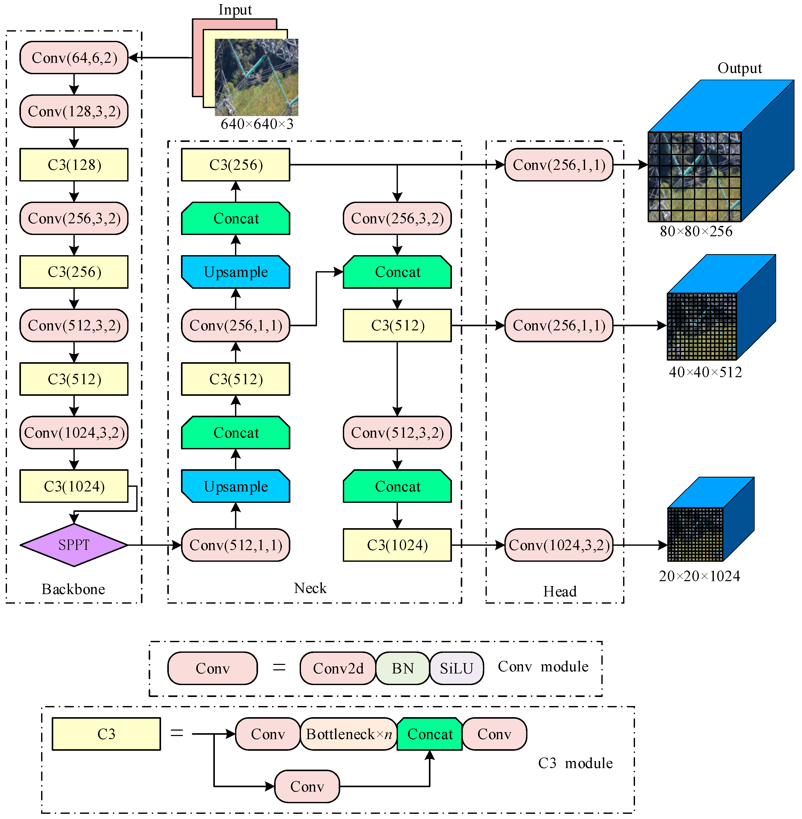
2.1. YOLOv5 Algorithm

YOLOv5 is a target detection algorithm further optimized and improved on the basis of YOLOv4. The YOLOv5 algorithm designs five different models for the depth and width of the module and the complexity of the model: YOLOv5n, YOLOv5s, YOLOv5m, YOLOv5l, and YOLOv5x, respectively, and the accuracy of the target detection of the five models is increased as the order of model complexity is sequentially increased. Among them, the complexity and accuracy of the YOLOv5s model is more balanced, so this paper chooses to use YOLOv5s as the basis for insulator defect detection.

The YOLOv5 target detection process has four parts, including the Input part, Backbone part, Neck part, and Head part, and the structure is shown in Figure 1.

When an input image with a pixel size of 640 × 640 is fed into the model, the Input part is enhanced with Mosaic data. The four insulator defect images are randomly cropped and stitched together to form a single image. The image is then preprocessed using adaptive anchor frame computation and adaptive image scaling operations.

The backbone network of YOLOv5 is CSPDarknet53, which contains the Focus module, CBL module, CSP1-x module, and SPP module [24]. This network primarily extracts target features by gradually reducing the size of the insulator defect map from 640 to 20. Additionally, the Focus and other modules slice the feature map, increasing the network depth and improving the effect of target feature extraction.

The Neck part primarily serves the purpose of feature extraction. The process of up-sampling and down-sampling is achieved through the use of an FPN (Feature Pyramid Net) and PAN (Path Aggregation Network) [25]. As shown in Figure 1, three sizes of feature maps, namely 2020, 4040, and 80 × 80, are obtained to facilitate the fusion of multiscale features.

The Head part receives the feature maps of different scales passed by the Neck part. It utilizes non-maximal value suppression to filter the target boxes and achieve the better recognition of multiple target checkboxes, thereby improving the prediction accuracy of the model.

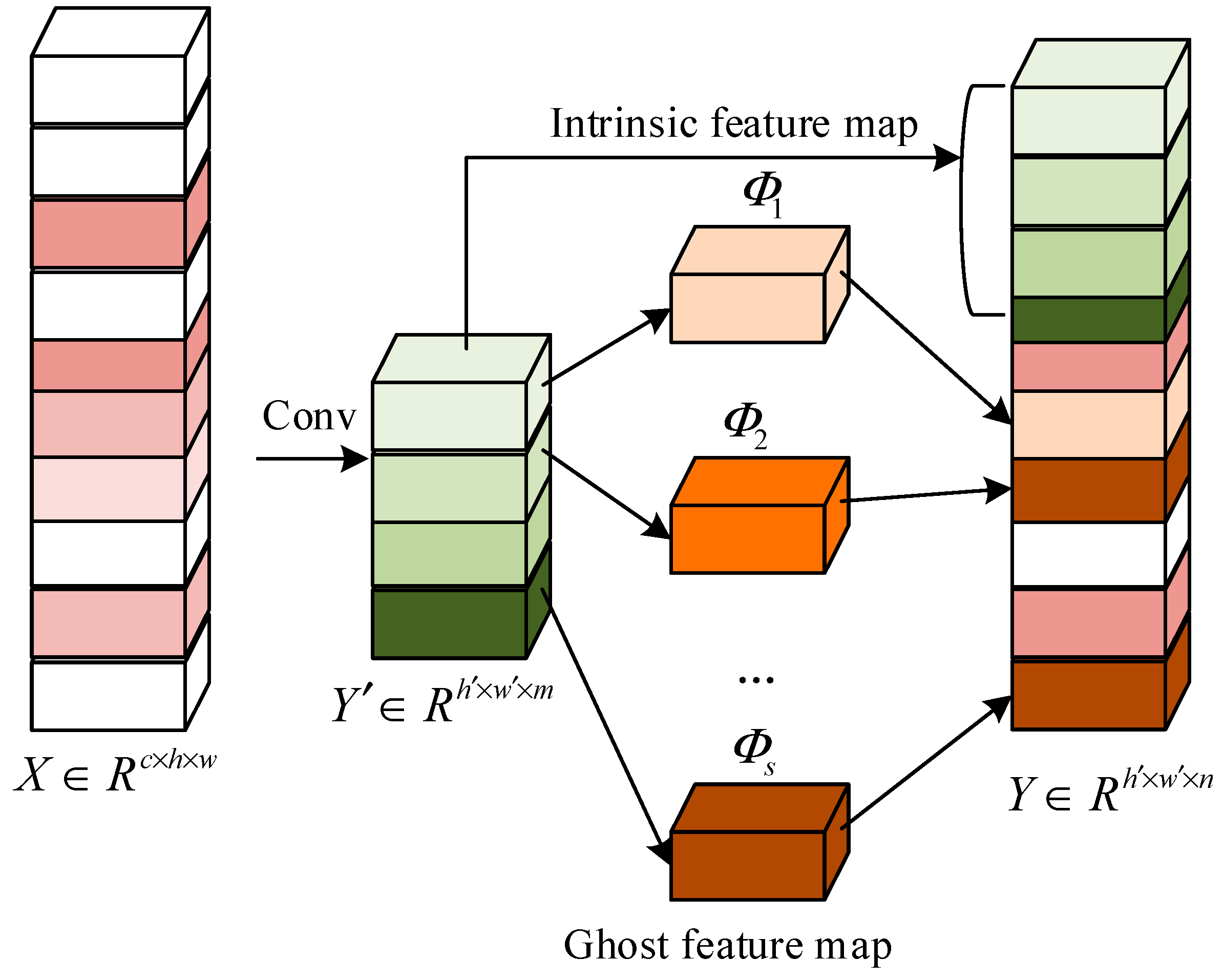
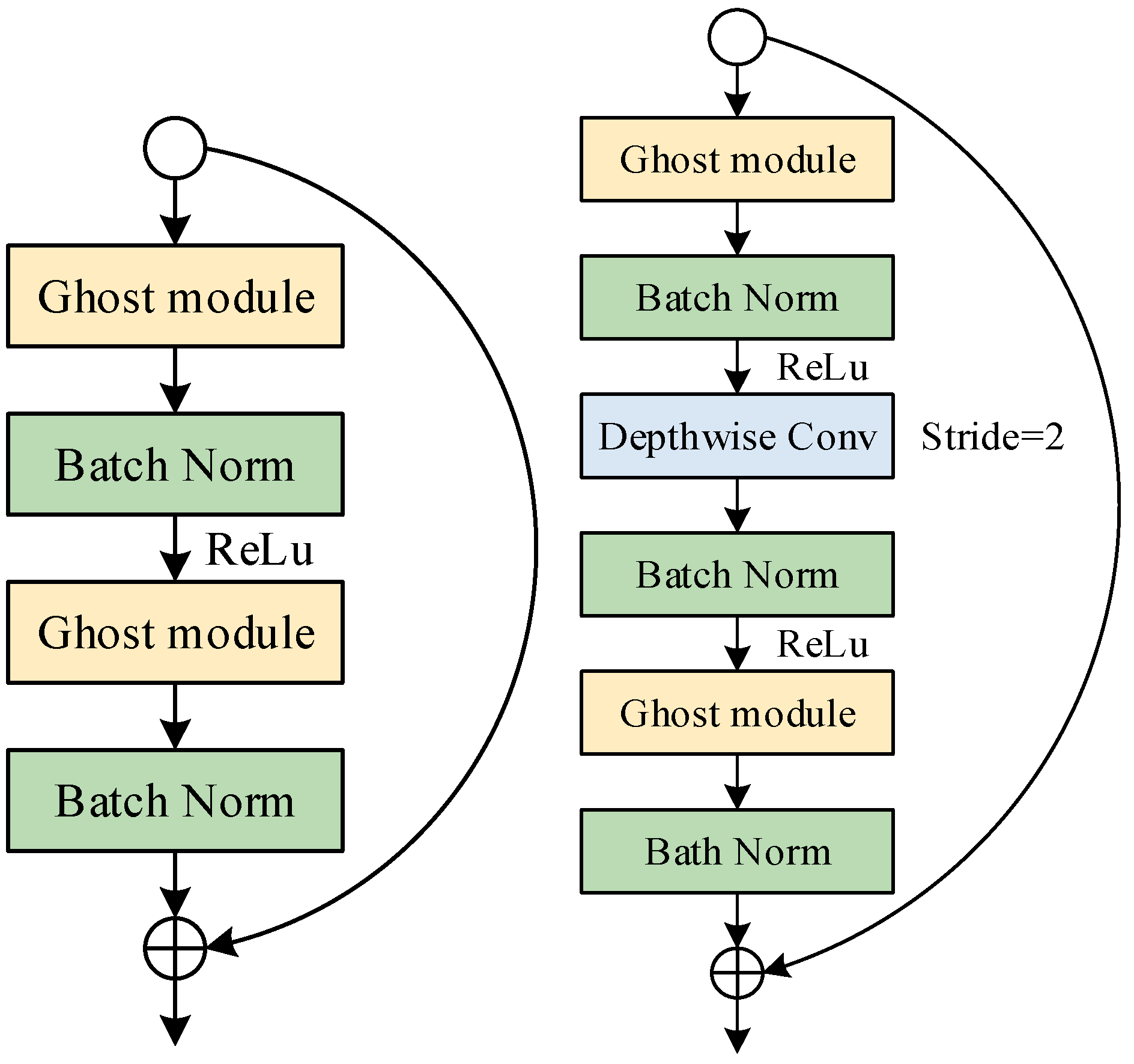
2.2. Lightweight Backbone GhostNet

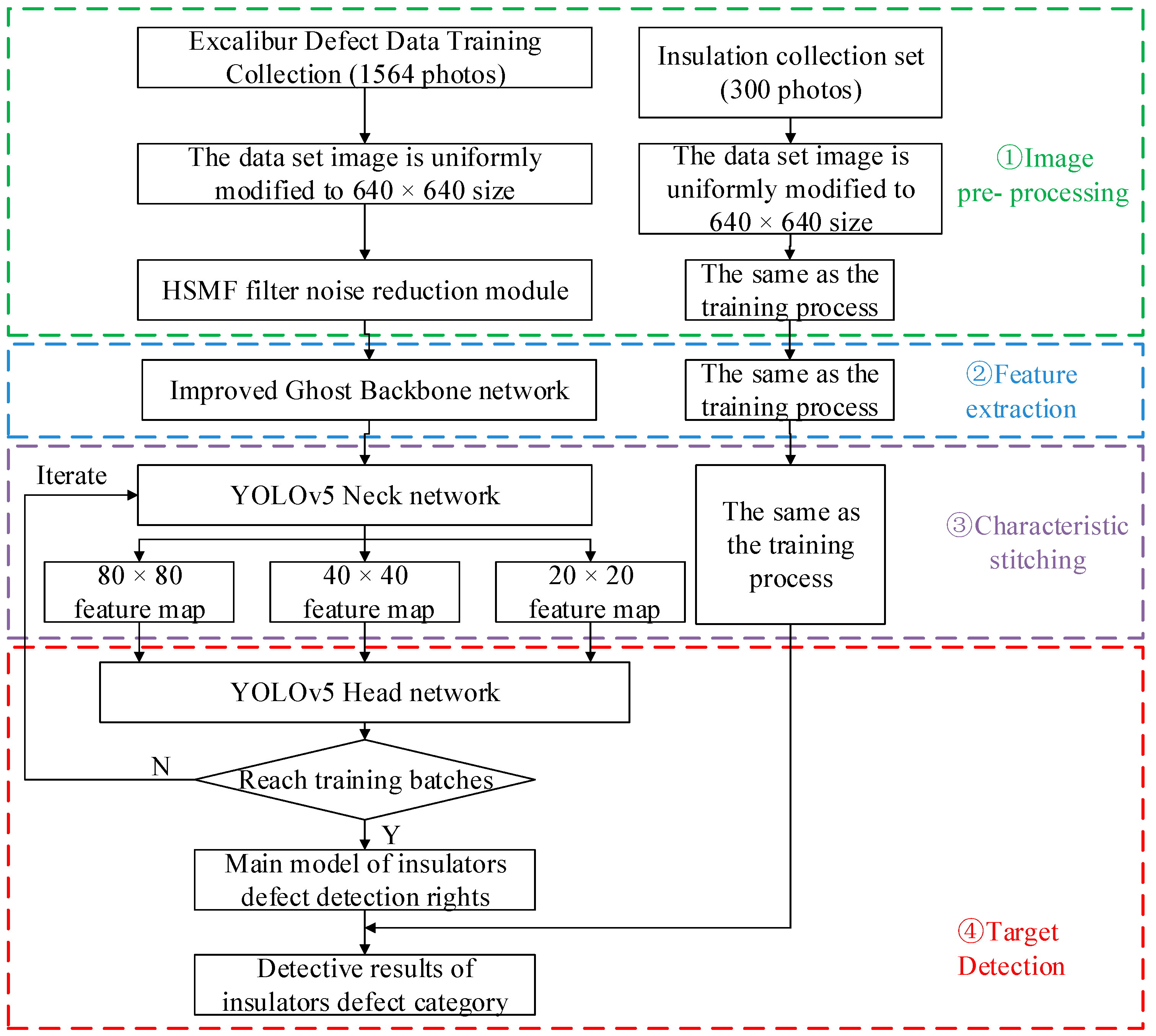
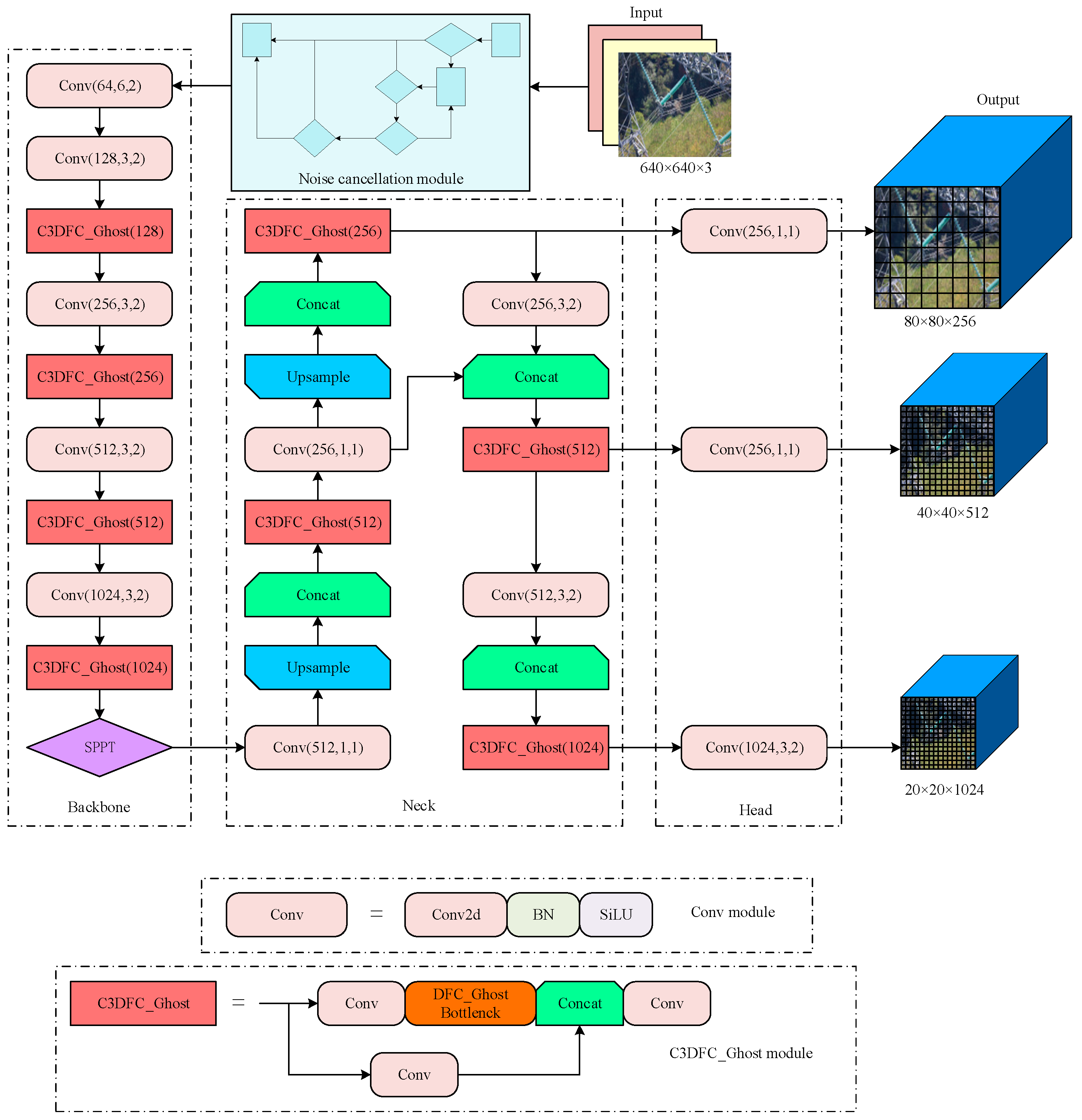
Although Backbone, the basis of YOLOv5, can efficiently extract target feature information, the network structure is too complex to be directly deployed on the Windows side, so the lightweight backbone network is the main direction for improvement at present. The GhostNet network model generates more feature maps using a smaller number of parameters, which is a clear advantage for the defect detection of targets [26]. The feature extraction process is shown in Figure 2.

The three parts of feature extraction can be analyzed based on the structure diagram:

The internal feature map is first obtained by regular convolution $Y_{w^{\prime }\ast h^{\prime }\ast m}$.

$$Y^{\prime }=X\ast f^{\prime }$$

(1)

in which $\ast$ represents the convolution operation, $Y^{\prime }\in {ℝ}^{h^{\prime }\times w^{\prime }\times \mathrm{m}}$ is the output feature map with m channels, $X$ denotes the input feature image, $f^{\prime }\in {ℝ}^{c\times k\times k\times m}$ is the convolution kernel used. $h^{\prime }$ and $w^{\prime }$ represent the height and width of the output feature map, respectively, $k\times k$ represents the number of kernels of the convolutional kernel, and $f^{\prime }$ represents the number of kernels.

Each individual channel of the $Y^{\prime }$ output is then represented by $y_i^{\prime }$, and the ${\mathsf{\Phi }}_{i,j}$ operation is employed to generate the Ghost feature map $y_{ij}^{}$; this process is as in Equation (2).

$$y_{ij}={\mathsf{\Phi }}_{i,j}\left(y_i^{\prime }\right),\forall i=1,\dots ,m,j=1,\dots ,s$$

(2)

where $y_i^{\prime }$ is the $Y^{\prime }$th original feature map in $i$, and ${\mathsf{\Phi }}_{i,j}$ in the above function is the $j$th linear operation for generating the $j$th Ghost feature map $y_{ij}$, $y_i^{\prime }$ may have one or more Ghost feature maps ${\left\{y_{ij}\right\}}_{j=1}^s$, and by ${\mathsf{\Phi }}_{i,s}$ preserving a constant mapping of the original feature maps.

Finally, the final feature stitching result is obtained by stitching (identity join) the ontology feature map with the Ghost feature map obtained in the second step.

Meanwhile, the principle of the Ghost module is utilized to design the Ghost Bottle neck layer, which is connected to the layer using the BN layer and nonlinearly activated using the ReLu activation function. For both Stride = 1 (left) and Stride = 2 (right) steps, the corresponding structures are represented in Figure 3.

3. DFCG_YOLOv5

When YOLOv5 is used for transmission line defect detection, there are issues such as slow algorithmic reasoning, a high misdetection rate for high-resolution images, and low accuracy when dealing with a large number of images and relatively small targets. To address these problems, this paper builds upon YOLOv5 and utilizes Ghost as the prototype for the backbone network. The backbone network is then improved. A network model called DFCG_YOLOv5, which combines joint denoising and lightweight target detection, is proposed. The overall detection process is illustrated in Figure 4.

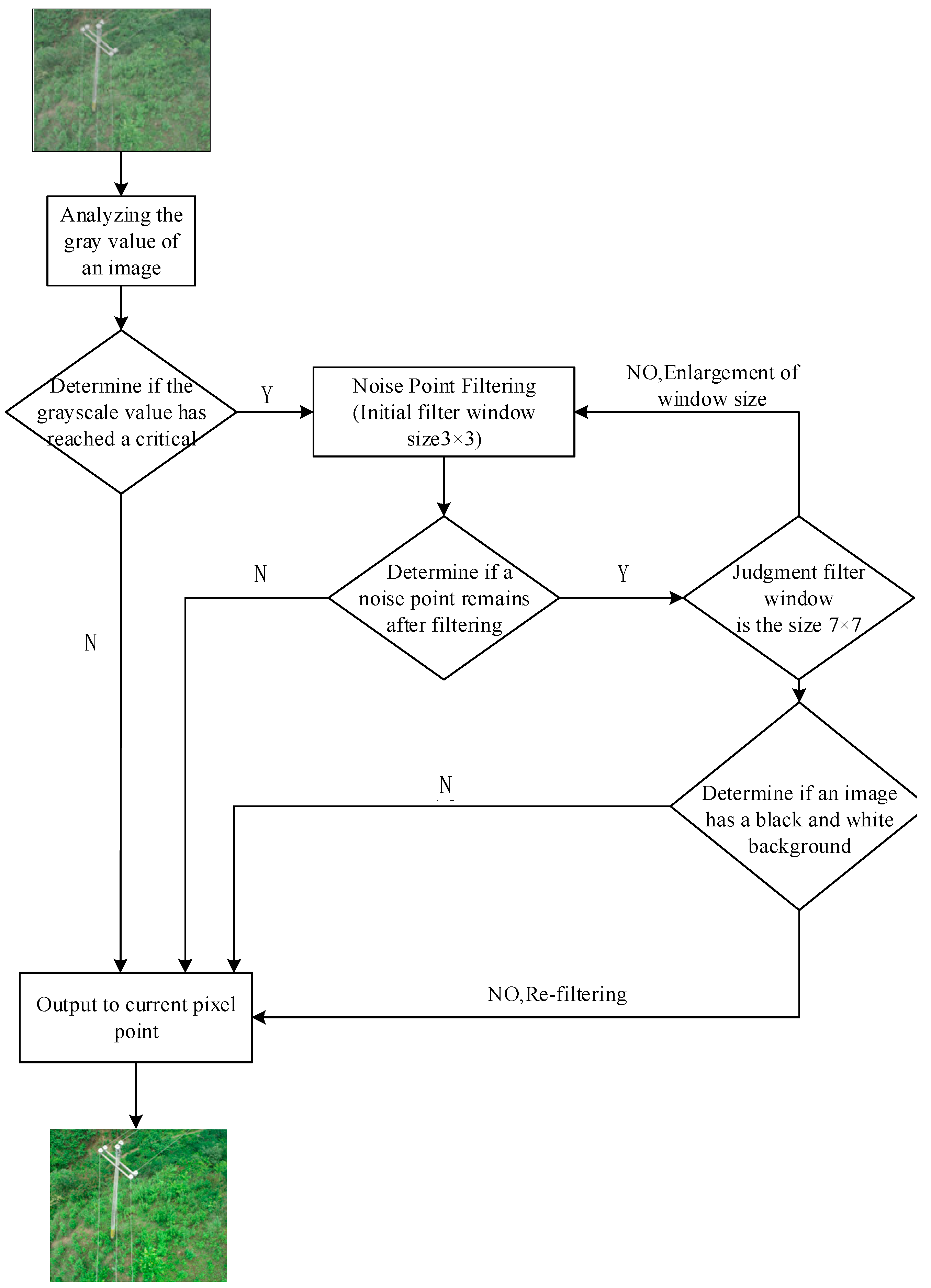
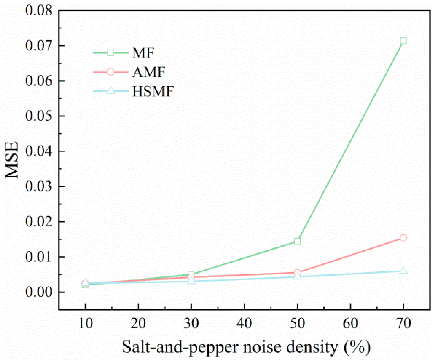
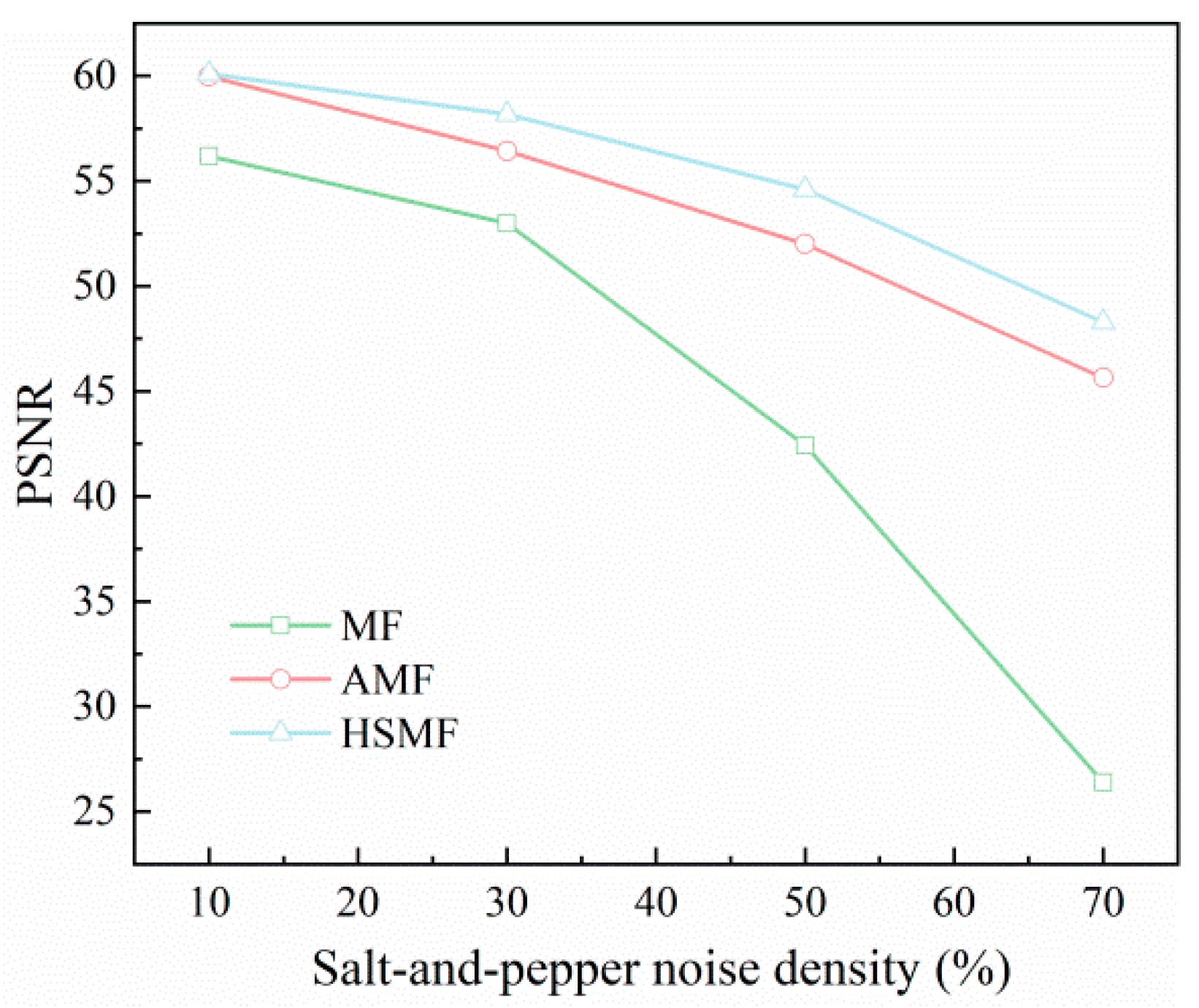
3.1. High-Speed Adaptive Median Filtering Algorithm HSMF

Based on the image quality transmitted by the UAV, it can be concluded that the quality of the image captured by the UAV will be affected by internal factors such as mechanical jitter and current instability, as well as external factors such as lighting conditions and weather. These factors can introduce incidental noise into the captured image. Therefore, it is necessary to add a noise reduction network to the Input part of YOLOv5 [27] to improve the preprocessing quality of the image. The most widely used filtering method for this purpose is the adaptive median filtering algorithm. The main process is as follows: firstly, according to the initial gray value, it can be divided into two processes: A and B; the pixel window corresponding to the pixel coordinate point $(i,j)$ of the image is set as $X(i,j)$, and the maximum size corresponding to the pixel window is set as $M_{\max }$; $Z_{\max }$, $Z_{\min }$, and $I_{\mathrm{med}}$ are set as the maximum, minimum, and median values of the corresponding window grayscale, respectively, and $Z(i,j)$ as the actual corresponding grayscale value of the coordinates. The A and B processes satisfy the following equation:

$$Z_{A1}=I_{\mathrm{med}}-Z_{\min }$$

(3)

$$Z_{A2}=Z_{\max }-I_{\mathrm{med}}$$

(4)

$$Z_{B1}=Z_{(i,j)}-Z_{\min }$$

(5)

$$Z_{B2}=Z_{\max }-Z_{(i,j)}$$

(6)

When the noisy image is transmitted to the filtering network, whether the image gray value is in the median range is analyzed, as in Equations (3) and (4). When the conditions are met, $Z_{A1}>0$ and $Z_{A2}>0$, the gray value is analyzed again and whether the gray value is in the threshold range of the set window gray value, if the gray value satisfies $Z_{B1}>0$ and $Z_{B2}>0$, then the pixel is judged as a pixel point. If it is not a non-noisy pixel point it will output the actual gray value $Z(i,j)$, or else it will output the median gray value $I_{\mathrm{med}}$.

However, in actual model detection, the traditional median filtering algorithm cannot meet the speed and effect demands of processing massive aerial images due to the high resolution and large number of pixels involved. To address this problem, this paper proposes a high-speed adaptive median filtering algorithm called HSMF. This algorithm classifies pixels into two categories: normal pixels and suspected noise pixels, based on the extreme value characteristics of noise. The algorithm retains normal pixel points while applying the high-speed adaptive median filtering algorithm to the suspected noise pixel points. It judges whether they are noise points according to the set median value, dynamically changes the window size of the median filter, and finally obtains the processed grayscale value.

The noise detection stage is first carried out by first setting the pixel gray value extremes of the image to represent the noise, using $Ma{x}_{gray}$ and $Mi{n}_{gray}$ to represent the maximum and minimum gray values corresponding to the noise, where $Ma{x}_{gray}$ = 255 is set and $Mi{n}_{gray}$ = 0 to indicate the gray value corresponding to the suspected noise pixel point.

$$Noise(i,j)=\{\begin{array}{l}0,x(i,j)=[\delta ,255-\delta ]\hfill \\ 1,\mathrm{otherwise}\hfill \end{array}$$

(7)

In Equation (7), $Noise(i,j)=1$ indicates that the point is a suspected noise pixel point, while $Noise(i,j)=0$ indicates that the point is a normal pixel point; $\delta$ represents the gray scale deviation, which is generally 1. In addition to the pixel points containing noise in the suspected noise pixel points, there are still some remaining normal pixel points with a gray value of 255 or 0, so it is still necessary to process the suspected noise points. The main process is as follows:

Use the initial $3\times 3$ filtering window to perform median filtering on the suspected noise pixel points, and determine whether there are any remaining suspected noise pixel points; if not, the noise filtering is over; if so, proceed to the next step.

Continue the filtering process by applying median filtering to the remaining pixel points from the previous step using the $5\times 5$ filter window.

The suspected noise pixel points remaining after filtering in the previous step $5\times 5$ are median filtered using the filtering window of $7\times 7$. It is judged whether the filtered noise still exists as suspected noise pixel points; if not, the noise filtering ends; if existing, it is classified and processed according to whether the image has a black and white background. If the image has a black and white background, the suspected noise points are considered to be the background part of the image, and the filtering process ends. If there is no black and white background, the remaining suspected noise pixel points are subjected to noise filtering in the $7\times 7$ filtering window. The overall process is shown in Figure 5.

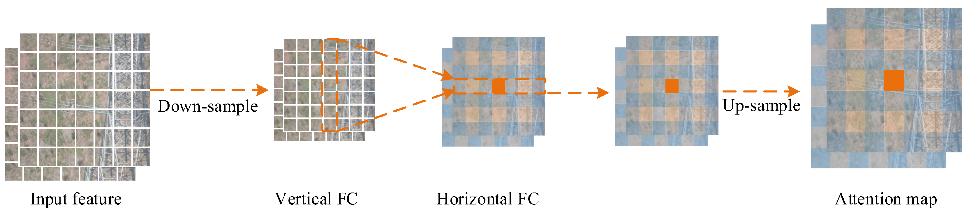
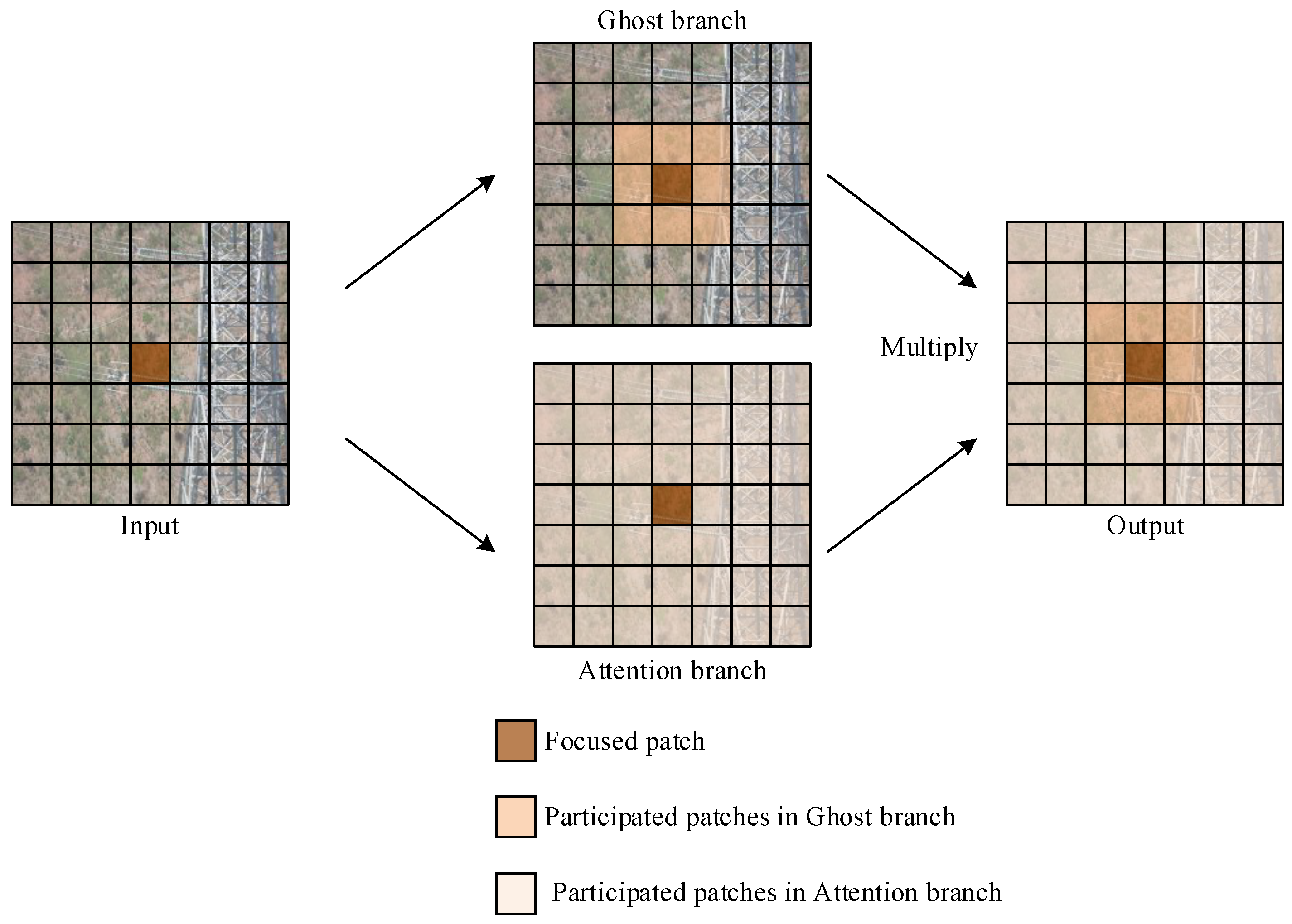
3.2. Decoupling the Fully Connected Attention Mechanism

Although the Ghost backbone network has met the requirements of the engineering deployment process in terms of a lightweight model, half of the spatial feature information is captured by the $3\times 3$ depth-wise convolution module and the remaining by the $1\times 1$ convolution module due to the oversimplification of its convolution structure. It cannot fulfill the practical application needs when dealing with high-resolution images like aerial images. Aiming at the current problem, this paper designs a decoupled fully connected attention mechanism (DFC Attention).

Assuming that the total number of features for a given image input is number $Z\in {ℝ}^{H\times W\times C}$ ($H$, $W$, and $C$ denote the image size as well as the number of channels, respectively), it can be viewed as $HW$ $z_i\in {ℝ}^C$,$Z\in \left\{z_{11},z_{12},\dots ,z_{HW}\right\}$. So, the fully connected layer (FC layer) with weights can be used to generate the attention feature map with global sensory field in the manner shown in Equation (8).

$$a_{hw}={\displaystyle \sum _{h^{\prime },w^{\prime }}{F}_{hw,h^{\prime },w^{\prime }}}\odot z_{h^{\prime },w^{\prime }}$$

(8)

where $\odot$ represents the multiplication of features and weights, $F$ is the FC layer learning weights, and $A=\left\{a_{11},a_{12},\dots ,a_{HW}\right\}$ is the generated attention feature map, but the computational complexity is quadratic with the image resolution $\mathcal{O}\left(H^2{W}^2\right)$, which is not suitable for aerial high-definition images. Therefore, this paper proposes to extract features from horizontal and vertical directions, respectively, as shown in Equations (9) and (10).

$$a_{hw}^{\prime }={\displaystyle \sum _{h^{\prime }=1}^H{F}_{h,h^{\prime }w}^H}\odot z_{h^{\prime }w},h=1,2,\cdots ,H,w=1,2,\cdots ,W$$

(9)

$$a_{hw}={\displaystyle \sum _{w^{\prime }=1}^W{F}_{w,h{w}^{\prime }}^W}\odot a_{h{w}^{\prime }}^{\prime },h=1,2,\cdots ,H,w=1,2,\cdots ,W$$

(10)

In Equations (9) and (10), $F^H$ and $F^W$ are the weights, and the input original features are $Z$. When the feature extraction part is carried out, Equations (9) and (10) are applied to the feature map in order to obtain the correlation from two directions, respectively, as in Figure 6.

This attention mechanism aggregates pixels at different locations according to horizontal and vertical directions, respectively, sharing a portion of the weights, which saves most of the inference time, and in order to be applicable to a variety of resolution images, the filter is decoupled from the size of the feature map, i.e., two deep convolutions of kernel sizes $1\times K_H$ and $K_W\times 1$ are performed sequentially on the input features, which theoretically turns the complexity into $O(K_{H}HW+K_{W}HW)$.

The Ghost module is augmented with the DFC attention mechanism to obtain the dependency of pixels in different spaces. When the image with feature $X\in R^{H\times W\times C}$ is input, it is divided into two partial branches, one part of the feature branch passes through the Ghost module and produces the output feature $Y$, and the other branch passes through the DFC attention module and produces the attention matrix $A$. The input $X$ is converted into the input of the DFC attention module through the $1\times 1$ convolution $Z$, and the final output of the product of the two branches is shown in Equation (11). The fusion process of the branch feature information is shown in Figure 7. The product is converted to the input of the DFC attention module, and the final output of the product of the two branches is shown in Equation (11). The fusion process of the two-branch feature information is shown in Figure 7.

$$O=\mathrm{Sigmoid}(A)\odot \mathcal{V}(X)$$

(11)

The Backbone structure uses DFC Attention branching in parallel with the Ghost branching module to enhance the extended features, which are then input to the second Ghost module to produce the output features. This is because the captured feature information is in different spatial locations and has dependency on each other, so the model’s expressive ability is greatly enhanced, and the structure is shown in Figure 7.

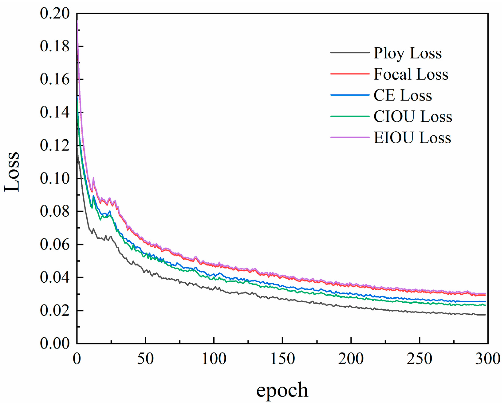
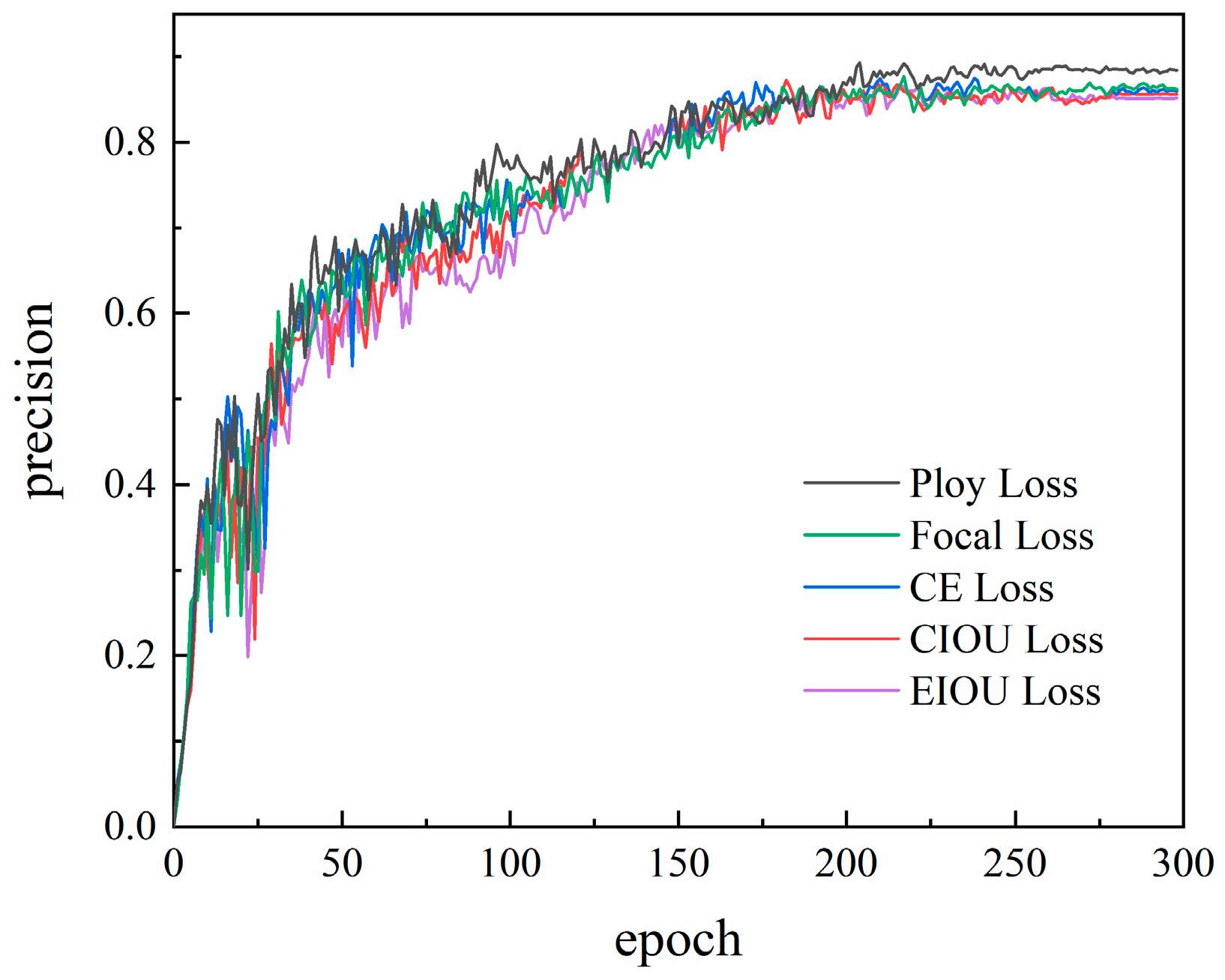
3.3. Loss Function Improvement

YOLOv5 mainly uses bounding box regression for target localization, which utilizes a rectangular bounding box to predict the position of the target object in the image, and refines the position of the bounding box in the process of continuous training. The bounding box regression uses the overlapping region between the predicted bounding box and the true bounding box as the loss function, which is called the IOU (Intersection over Union) loss function [28], as in Equation (12).

$$IOU=\frac{A\cap B}{A\cup B}$$

(12)

In Equation (12), A represents the area of the predicted bounding box and B represents the area of the real bounding box, IOU can measure the degree of overlap, but the rest of the target information cannot be judged, and there is no convergence effect in the case where the predicted box does not intersect with the real box with an area of zero. Later, GIOU Loss was introduced to solve this problem [29], but the computational volume is relatively large and the convergence speed is slow. DIOU Loss utilizes the distance between the real bounding box and the predicted bounding box as the convergence index of the loss function, which improves the detection effect [30]. CIOU Loss introduces the aspect ratio of the real bounding box to the predicted bounding box and achieves relatively good convergence results [31], but it is not applicable to target detection for datasets such as UAV aerial images, and there is no targeted strategy for the serious imbalance of positive and negative samples present in small targets. There is no targeted strategy.

In this paper, we propose a loss function, Poly Loss, which can be adjusted to the positive and negative sample coefficients for different datasets. Firstly, the commonly used two types of loss functions (Cross Entropy Loss Function and Focal Loss) are expanded by Taylor Decomposition, as shown in Equation (13).

$${\Sigma }_{j=1}^{+\infty }{\alpha }_j{\left(1-P_t\right)}^j$$

(13)

In Equation (13), ${\alpha }_j\in R^{+}$ represents the weight coefficients of the polynomial and $P_t$ the probability of target label prediction. Its engineering applicability is mainly reflected in the application to different scenarios and the fact that different datasets can make the loss function more suitable for the target recognition task by adjusting the polynomial coefficients, ${\alpha }_j$.

And it can be concluded from the calculation that the effect of adjusting the first polynomial coefficient of the Taylor expansion polynomial term, Poly_L1, has been superior to that of the cross-entropy loss function with the Focal Loss, which is expressed as in Equation (14).

$$L_{\mathrm{Poly}\text{\_}L1}=\left(1+{ϵ}_1\right)\left(1-P_t\right)+1/2{\left(1-P_t\right)}^2+\dots =-\log \left(P_t\right)+{ϵ}_1\left(1-P_t\right)$$

(14)

To address the problem of positive and negative sample imbalance in small target datasets, one approach is to adjust the polynomial coefficients of the positive samples suppression. This tuning parameter is simple to adjust and can be flexibly modified for different datasets, thereby improving the model’s effectiveness.

The overall network structure diagram of the improved DFCG_YOLOv5 algorithm is presented in Figure 8. By optimizing the C3 module in the YOLOv5 Backbone using the enhanced DFC_Ghost network structure, the feature map utilization is increased while interference from irrelevant information is reduced, leading to the improved accuracy and robustness of the network. To provide a more detailed illustration of the network architecture, this paper includes simplified code for the target detection process in Appendix A. In the first step, the insulator defect image is uniformly cropped to a size of 640 × 640 × 3 through preprocessing. Different sizes of anchor frames are then generated, and the image is input into the improved DFC_Ghost backbone network to produce three feature maps with varying scales. These feature maps are used to predict whether each grid cell contains a target, the class of the target, as well as the target’s location and size. The cross-entropy loss is then computed using the Poly Loss function to obtain the accurate probability of insulator defect small target predictions. Additionally, the Poly term is introduced to amplify the penalty for incorrect probabilities and enhance the contribution of correct probabilities. Subsequently, bounding boxes with confidence below a certain threshold are eliminated, and the non-maximum suppression algorithm is utilized to remove overlapping bounding boxes. The final results are then generated. In references [32,33,34], the improved Ghost network is also combined with the YOLO algorithm and applied to industrial defect detection, resulting in enhanced accuracy. This further validates the effectiveness of the algorithm proposed in this paper.

4. Experimental Results and Analysis

4.1. Experimental Environment and Evaluation Indicators

4.1.1. Experimental Environment

In order to ensure the engineering applicability of the algorithm, the datasets used in this paper were all downloaded from the unmanned aircraft system of Yunnan Power Supply Company, Jinghong, China. The images were all taken by the UAV at a height of 3–4 metres from the transmission line, with a maximum resolution of 8688 × 5792, and 1864 insulator defect images were selected after screening, including four types of defects: insulator breakage, insulator self-detonation, insulator fouling, and insulator tie line loosening, and the defect labels are set as “jyzps, jyzzb, jyzwh, and jyzzxst”, respectively. For each class of defects, 75 images are selected as the validation set and the remaining are used as the training set. According to previous manual screening experience, the ratio of normal insulator images to defective insulator images is about 10:1, so in this paper, in order to be more in line with the actual application scenarios, the remaining 3124 normal insulator images are also added to the validation set, and the number of defects in each class and the distribution of the training and validation sets are shown in Figure 9.

The YOLOv5s architecture was employed to train the model via basic training, with a batch size of 32 and 300 training batches. The initial learning rate was set to 0.01, the momentum factor was set to 0.937, and the weight decay coefficient was set to 0.0005. The stochastic gradient descent (SGD) method was utilized for optimization. The experimental platform environment is illustrated in

Table 1. Experimental platform environment configuration.

Environmental Configuration	Parameter
operating system	Window10
GPU	NVIDIA Quadro P4000(8 G)
CPU	Intel(R) Core (TM)i9-9900K
deep learning model framework	Pytorch 1.7.1
GPU acceleration environment	CUDA 11.0.2
programming language	Python3.8

.

4.1.2. Evaluation Index

In order to quantitatively judge the image denoising effect from an objective point of view, this paper selects the mean square error (MSE) and the Peak Signal to Noise Ratio (PSNR) as the quantitative evaluation indexes. PSNR is an objective evaluation method in the field of an image, which is usually defined by the mean square error (MSE) of the image, as shown in Equation (15).

$$MSE=\frac{1}{\mathrm{mn}}{\displaystyle \sum _{i=0}^{\mathrm{m}-1}{\displaystyle \sum _{j=0}^{\mathrm{n}-1}{\Vert I\left(i,j\right)-K\left(i,j\right)\Vert }^2}}$$

(15)

where m, n represent the height and width of the image, respectively, $I\left(i,j\right)$ and $K\left(i,j\right)$ represent the pixel values with coordinates $\left(i,j\right)$ before and after the image is filtered, respectively. The signal to noise ratio is defined as in Equation (16).

$$PSNR=10\cdot {\log }_{10}\left(\frac{MA{X}_I^2}{MSE}\right)$$

(16)

In the formula, MAX represents the maximum pixel value of the image and MSE is the mean square error value.

And Precision, Recall, and mAP are used as the relevant indexes to evaluate the performance of the target detection model. Precision is used to measure the accuracy of the classification detection of the model and is denoted as P. Recall measures whether the model detects comprehensively or not and is denoted as R. The area under the curve plotted by Precision and Recall is the value of AP. MAP represents the average value of AP for each category. The mAP value is generally calculated at IOU = 0.5, i.e., mAP@0.5, as in Equations (17)–(20).

$$Precise=\frac{TP}{TP+FP}$$

(17)

$$Recall=\frac{TP}{TP+FN}$$

(18)

$$AP={\displaystyle {\int }_0^{1}P}(r)\mathrm{d}r$$

(19)

$$mAP=\frac{{\displaystyle \sum _{i=1}^{C}A}{P}_i}{C}$$

(20)

where TP denotes correctly predicted positive samples as positive, FN denotes incorrectly predicted positive samples as negative, and FP denotes incorrectly predicted negative samples as positive; and C represents the type of target detection.

4.2. Comparison of Ablation Experiments

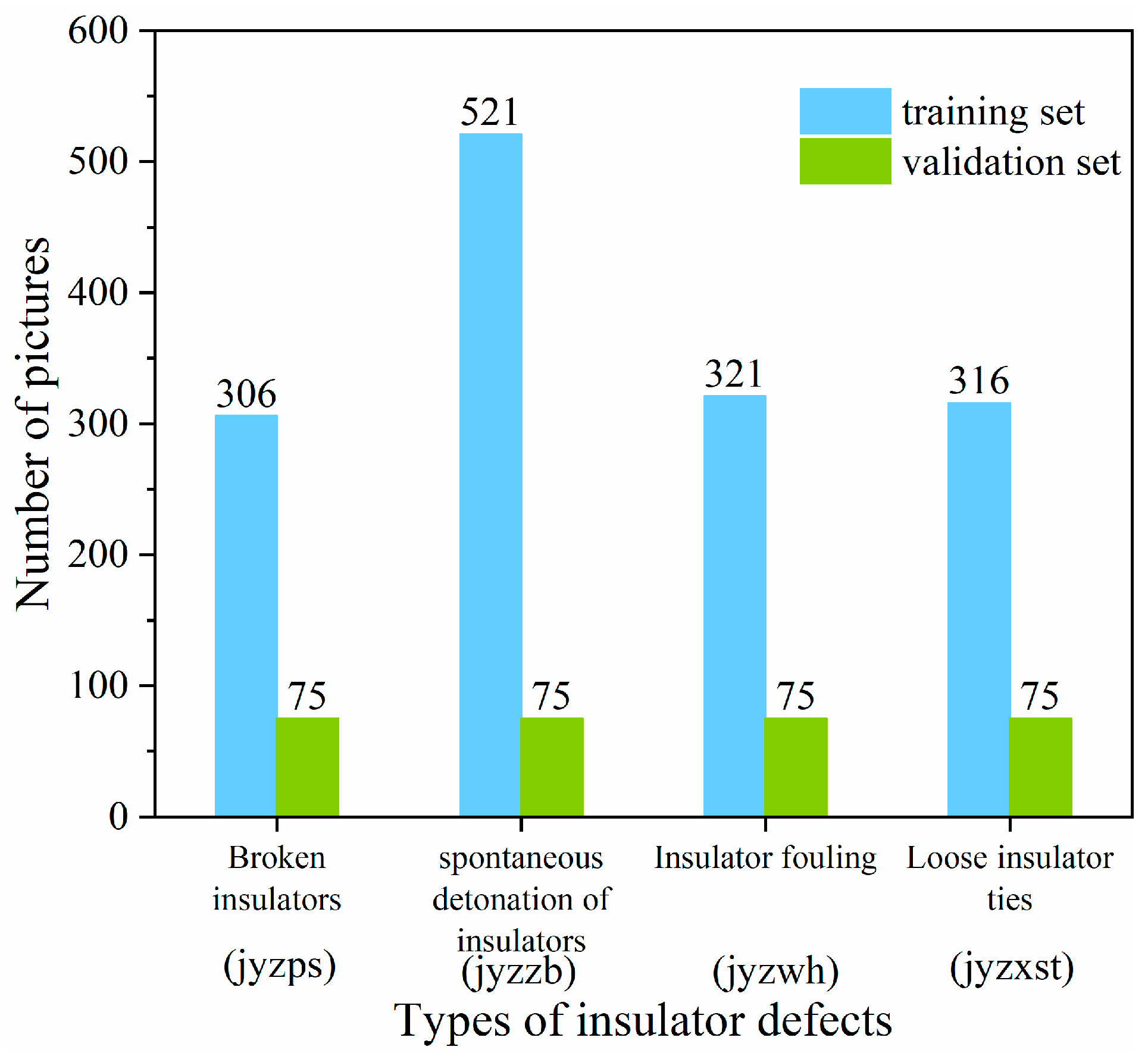
4.2.1. Input Section to Add HSMF Noise Reduction Network Effect

In order to verify the effect of the UAV aerial images on target detection, this experiment adds pretzel noise with noise densities of 0.1, 0.3, 0.5, and 0.7 to all the datasets, respectively, and verifies the effect of noise on the detection results, as shown in

Table 2. Effect of different levels of noise on YOLOv5 detection.

Noise Density	(all) P	(all) R	(all) mAp@0.5	(all) mAp@0.5:0.95
0	0.856	0.743	0.805	0.596
0.1	0.821	0.740	0.759	0.571
0.3	0.814	0.732	0.747	0.570
0.5	0.803	0.721	0.736	0.567
0.7	0.801	0.703	0.729	0.561

.

According to Table 2, it can be concluded that the unprocessed incidental noise images have a significant impact on image detection. When the image is subjected to a pretzel noise density of 0.1, the overall accuracy of all the types of defects decreases by an average of 3.5%, and the overall performance decreases by 0.46. Additionally, with every increase of 0.2 in the noise density, the overall accuracy decreases by an average of about 1%, and the overall performance decreases by approximately 0.01. The results of when the noisy image is processed using HSMF (High-Speed Median Filtering) are depicted in Figure 10 and Figure 11.

After processing the aerial images with a pretzel noise density of 0.1, 0.2, 0.3, and 0.4, respectively, using HSMF algorithm, the target detection experiments are re-conducted and the results are shown in

Table 3. Noise reduction effect of different densities.

Noise Reduction Rating	(all) P	(all) R	(all) mAp@0.5	(all) mAp@0.5:0.95
0.1	0.849	0.742	0.789	0.589
0.3	0.840	0.730	0.778	0.584
0.5	0.836	0.732	0.769	0.583
0.7	0.825	0.726	0.760	0.581

.

The experimental results in Table 3 verify that there is a significant improvement in the image detection after processing by the HSMF filter module, with an average increase in accuracy of about 2.5% and a 0.03 growth in the overall performance mAP, which verifies the necessity of the improvement of the image preprocessing part.

4.2.2. Improvement of the Loss Function

Before verifying the effect of the Ploy Loss function, the hyperparameter ${ϵ}_1$ needs to be adjusted to make it more compatible with the number set constructed in this paper, so as to improve the convergence of the model. The ablation experiments are shown in

Table 4. Detection performance for different parameter values.

${\mathit{ϵ}}_1$ Parameter Value	(all) P	(all) R	(all) mAp@0.5	(all) mAp@0.5:0.95
1	0.862	0.772	0.749	0.605
3	0.874	0.765	0.754	0.609
5	0.883	0.756	0.769	0.612
7	0.877	0.739	0.762	0.607
9	0.869	0.755	0.754	0.604

.

Based on the ablation experiments, it can be concluded that the loss function is more compatible with the dataset when the hyperparameter ${ϵ}_1=5$. At this time, the probability penalty for prediction error is moderate, the positive and negative sample balance is optimal, and the loss function converges best.

In order to verify the applicability of Poly Loss engineering, the experiment conducted with YOLOv5 comes with better performance loss functions: CIOU Loss and EIOU Loss [35] as well as Focal Loss [36] and CE Loss (Cross Entropy Loss) [37] for adapting small targets for ablation experiments, respectively. The experimental results are shown in

Table 5. Graph of detection effect of different loss functions.

Type of Loss Function	(all) P	(all) R	(all) mAp@0.5	(all) mAp@0.5:0.95
CIOU Loss	0.856	0.743	0.751	0.596
EIOU Loss	0.851	0.731	0.742	0.592
CE Loss	0.862	0.736	0.759	0.599
Focal Loss	0.859	0.742	0.752	0.592
Ploy Loss	0.883	0.756	0.769	0.612

, Figure 12 and Figure 13.

By examining the chart, it can be observed that YOLOv5’s own loss functions, namely CIOU Loss and EIOU Loss, have a relatively low accuracy for small target detection and a poor overall performance. On the other hand, Ploy Loss performs better in addressing the imbalance between the positive and negative samples in an image, and achieves higher accuracy and better overall performance compared to Focal Loss and CE Loss. Additionally, Ploy Loss has a more prominent convergence speed and effect, making it more applicable to engineering.

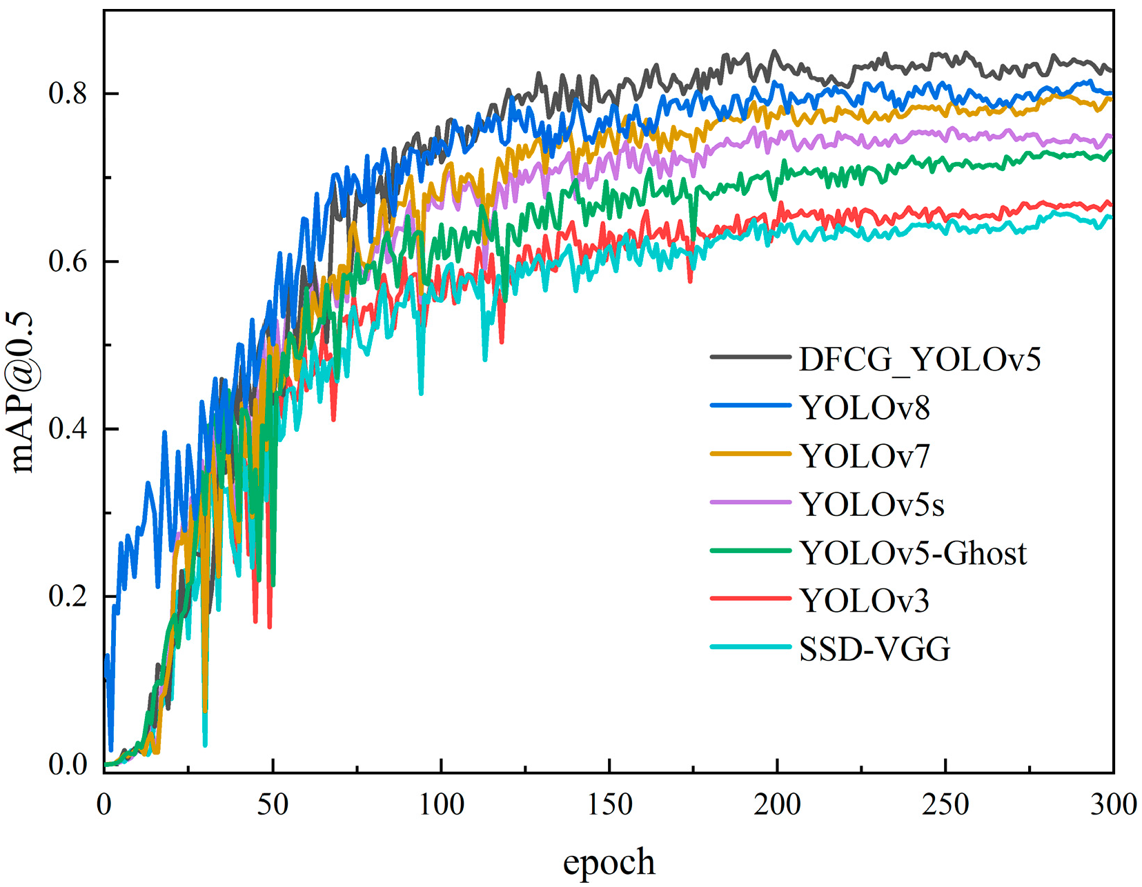
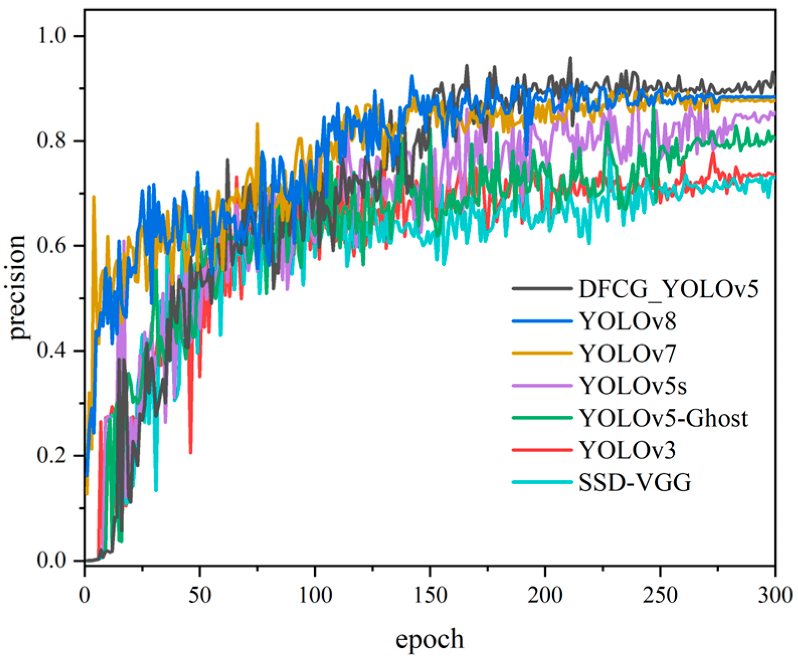
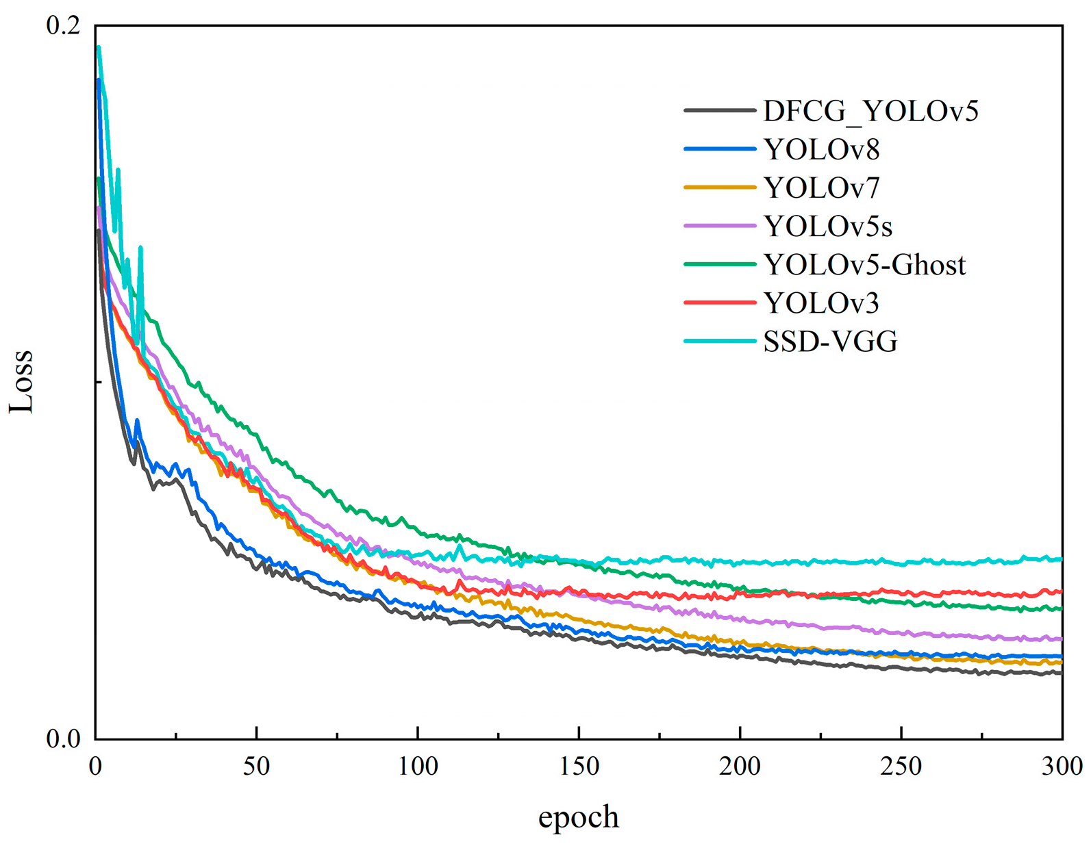
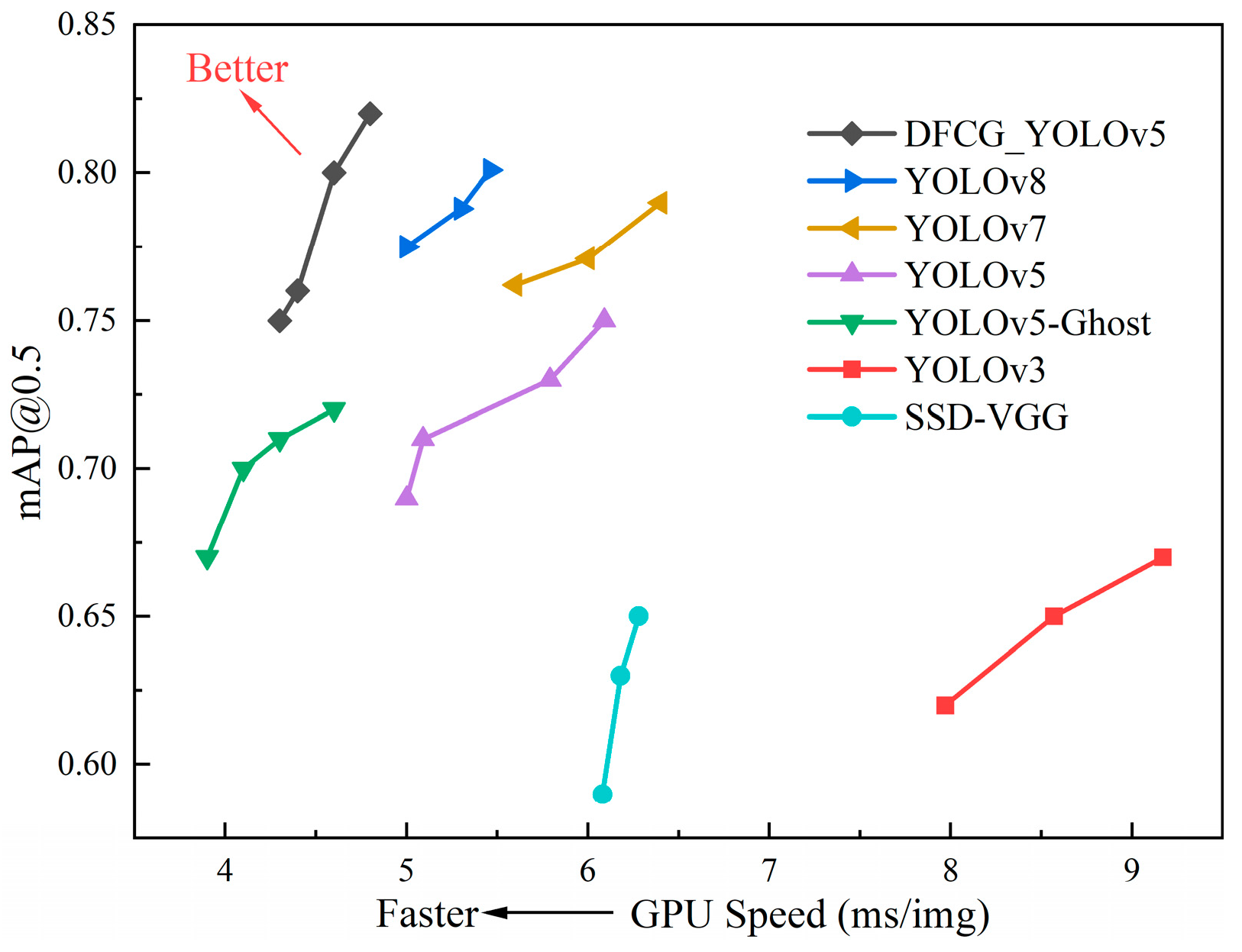
4.2.3. DFCG_YOLOv5 Overall Detection Effect

In order to verify the effectiveness of the improved overall algorithm as the backbone network of DFC Ghost, the improved algorithm is compared with the more widely used target detection algorithms such as the basic networks YOLOv5s and YOLOv5m, YOLOv5-Ghost, YOLOv3 [38], SSD-VGG [39], YOLOv6m [40], and the newest algorithms YOLOv7 [41] and YOLOv8 [42], etc., and the results are shown in

Table 6. Comparison of target detection performance.

Method	(all) P	(all) R	(all) mAp@0.5	FPS (Hz)
YOLOv3	0.734	0.628	0.666	109
SSD-VGG	0.728	0.636	0.651	159
YOLOv5s	0.856	0.743	0.751	139
YOLOv5m	0.863	0.721	0.779	102
YOLOv5-Ghost	0.803	0.692	0.727	218
YOLOv6m	0.871	0.716	0.791	112
YOLOv7	0.879	0.738	0.792	155
YOLOv8	0.885	0.741	0.801	183
DFCG_YOLOv5	0.899	0.748	0.822	207

. The comprehensive performance comparison of each type of algorithm is shown in Figure 14, the accuracy of each type of algorithm as well as the convergence effect is shown in Figure 15 and Figure 16, and finally, Figure 17 is used to indicate the degree of balance between the accuracy and speed of each type of algorithm (the gap between YOLOv5m and YOLOv6m is relatively small, and is not shown in the figure).

Figure 14 clearly demonstrates the superior overall performance of the DFCG_YOLOv5 algorithm compared to other algorithms (mAP). In addition, Figure 15 and Figure 16 show that DFCG_YOLOv5 achieves the highest accuracy and most robust convergence under complex conditions. Finally, Figure 17 visually demonstrates the superiority of DFCG_YOLOv5 in terms of speed and accuracy compared to other algorithms.

Furthermore, in terms of effectiveness, the algorithm proposed in this paper exhibits fewer false and missed detections in the detection of 300 insulator defect maps compared to other algorithms. This feature makes it more suitable for engineering applications. Examples of various types of defect detection are shown in Figure 18.

5. Discussion

Based on the analysis of the experimental results in Figure 13, the algorithm DFCG_YOLOv5 (0.822) proposed in this manuscript shows superior overall performance (mAP) compared to the benchmark network YOLOv5-Ghost (0.727) and the base algorithms YOLOv5s (0.751) and YOLOv5m (0.779). Not only is it superior to the traditional algorithms YOLOv3 (0.666) and SSD (0.651), but in addition, compared to the latest algorithms, the algorithm’s performance is improved by 3.9% compared to YOLOv6m (0.791), 3.7% compared to YOLOv7 (0.792), and 2.6% compared to YOLOv8 (0.801), validating the DFCG_YOLOv5 algorithm’s advantages. In terms of accuracy, the algorithm in this paper not only far outperforms YOLOv3 (0.734) and SSD (0.728), but also outperforms the benchmark algorithms YOLOv5s (0.856) and YOLOv5m (0.863), as well as the benchmark network, YOLOv5-Ghost (0.803), which demonstrates a clear advantage. Its accuracy is 3.1%, 2.2%, and 1.6% higher than the latest algorithms YOLOv6m, YOLOv7, and YOLOv8, respectively. In terms of speed, based on Figure 16, it can be concluded that the algorithm proposed in this paper has a significant advantage with an improvement of 84% compared to YOLOv6m, 33.5% compared to YOLOv7, and 13.1% compared to YOLOv8. This is visually depicted in Figure 17, which clearly illustrates that the algorithm proposed in this paper achieves an excellent balance between accuracy and speed.

According to the actual verification set results, 300 insulator defect images and 279 defects were detected, with a leakage rate of 7%, and 101 out of 3124 normal insulator images were misdetected as images containing defective insulators, with a misdetection rate of 3.2%, which is fully in line with the application requirements of actual industrial scenarios.

6. Conclusions

Building upon the YOLOv5 algorithm with the lightweight Ghost network as its foundation, this study introduces the DFCG_YOLOv5 algorithm, which combines adaptive median filtering for noise reduction and lightweight target detection. To enhance the filtering capability for aerial images of varying quality, an optimized version of the traditional median filtering algorithm called HSMF (High-Speed Median Filtering) is proposed. Furthermore, in order to balance accuracy and speed, structural improvements are made to the lightweight Ghost backbone network, ensuring improved accuracy without compromising inference speed, thus better addressing the complexities of practical application scenarios. To enhance the detection of small targets, the Poly Loss classification loss function is employed to tackle the issue of imbalanced positive and negative samples by adjusting the parameters and suppressing positive samples. Finally, the dataset utilized in this research consists of machine patrol images obtained from the power supply company’s UAV system, thus providing a more robust validation of the algorithm’s applicability to real-world projects.

In the future, the focus will be on two main areas. Firstly, the limited availability of the transmission line defects dataset due to confidentiality concerns hinders further model optimization. To address this, a plan is in place to design an interface using pyqt5 and package it as an application for deployment in the power supply bureau. This will enable the iterative optimization of the model. In addition, there will be further optimization of the network structure to incorporate targeted strategies for detecting small targets. This optimization aims to improve detection performance, achieving the real-time and efficient identification of transmission line defects.

References

1. Taqi, A.; Beryozkina, S. Overhead transmission line thermographic inspection using a drone. In Proceedings of the 2019 IEEE 10th GCC Conference & Exhibition (GCC), Kuwait, Kuwait, 19–23 April 2019; pp. 1–6. [Google Scholar]
2. Hao, J.; Zhou, Y.; Zhang, G. A review of target tracking algorithm based on UAV. In Proceedings of the 2018 IEEE International Conference on Cyborg and Bionic Systems (CBS), Shenzhen, China, 25–27 October 2018; pp. 328–333. [Google Scholar]
3. Girshick, R.; Donahue, J.; Darrell, T.; Malik, J. Rich feature hierarchies for accurate object detection and semantic segmentation. In Proceedings of the IEEE Conference on Computer Vision and Pattern Recognition, Columbus, OH, USA, 23–28 June 2014; pp. 580–587. [Google Scholar]
4. Girshick, R. Fast r-cnn. In Proceedings of the IEEE International Conference on Computer Vision, Santiago, Chile, 7–13 December 2015; pp. 1440–1448. [Google Scholar]
5. Ren, S.; He, K.; Girshick, R.; Sun, J. Faster r-cnn: Towards real-time object detection with region proposal networks. Adv. Neural Inf. Process. Syst. 2015, 28. [Google Scholar] [CrossRef] [PubMed]
6. Xu, X.; Zhao, M.; Shi, P.; Ren, R.; He, X.; Wei, X.; Yang, H. Crack detection and comparison study based on faster R-CNN and mask R-CNN. Sensors 2022, 22, 1215. [Google Scholar] [CrossRef] [PubMed]
7. Yao, L.; Zhang, N.; Gao, A.; Wan, Y. Research on Fabric Defect Detection Technology Based on EDSR and Improved Faster RCNN. In Proceedings of the International Conference on Knowledge Science, Engineering and Management, Singapore, 6–8 August 2022; Springer International Publishing: Cham, Switzerland, 2022; pp. 477–488. [Google Scholar]
8. Ni, H.; Wang, M.; Zhao, L. An improved Faster R-CNN for defect recognition of key components of transmission line. Math. Biosci. Eng. 2021, 18, 4679–4695. [Google Scholar] [CrossRef] [PubMed]
9. Huang, Z.; Wang, J.; Fu, X.; Yu, T.; Guo, Y.; Wang, R. DC-SPP-YOLO: Dense connection and spatial pyramid pooling based YOLO for object detection. Inf. Sci. 2020, 522, 241–258. [Google Scholar] [CrossRef]
10. Redmon, J.; Divvala, S.; Girshick, R.; Farhadi, A. You only look once: Unified, real-time object detection. In Proceedings of the IEEE Conference on Computer Vision and Pattern Recognition, Las Vegas, NV, USA, 26 June–1 July 2016; pp. 779–788. [Google Scholar]
11. Zhang, X.; Zhang, L.; Li, D. Transmission line abnormal target detection based on machine learning yolo v3. In Proceedings of the 2019 IEEE International Conference on Advanced Mechatronic Systems (ICAMechS), Shiga, Japan, 26–28 August 2019; pp. 344–348. [Google Scholar]
12. Zeng, T.; Li, S.; Song, Q.; Zhong, F.; Wei, X. Lightweight tomato real-time detection method based on improved YOLO and mobile deployment. Comput. Electron. Agric. 2023, 205, 107625. [Google Scholar] [CrossRef]
13. Ding, X.; Zhang, X.; Ma, N.; Han, J.; Ding, G.; Sun, J. Repvgg: Making vgg-style convnets great again. In Proceedings of the IEEE/CVF Conference on Computer Vision and Pattern Recognition, Nashville, TN, USA, 20–25 June 2021; pp. 13733–13742. [Google Scholar]
14. Li, L.; Wang, Z.; Zhang, T. Gbh-yolov5: Ghost convolution with bottleneckcsp and tiny target prediction head incorporating yolov5 for pv panel defect detection. Electronics 2023, 12, 561. [Google Scholar] [CrossRef]
15. Gao, J.; Chen, X.; Lin, D. Insulator defect detection based on improved YOLOv5. In Proceedings of the 2021 5th IEEE Asian Conference on Artificial Intelligence Technology (ACAIT), Haikou, China, 29–31 October 2021; pp. 53–58. [Google Scholar]
16. Zhang, T.; Zhang, Y.; Xin, M.; Liao, J.; Xie, Q. A Light-Weight Network for Small Insulator and Defect Detection Using UAV Imaging Based on Improved YOLOv5. Sensors 2023, 23, 5249. [Google Scholar] [CrossRef]
17. Hao, K.; Chen, G.; Zhao, L.; Li, Z.; Liu, Y.; Wang, C. An insulator defect detection model in aerial images based on multiscale feature pyramid network. IEEE Trans. Instrum. Meas. 2022, 71, 3522412. [Google Scholar] [CrossRef]
18. Cao, Z.; Mei, F.; Zhang, D.; Liu, B.; Wang, Y.; Hou, W. Recognition and Detection of Persimmon in a Natural Environment Based on an Improved YOLOv5 Model. Electronics 2023, 12, 785. [Google Scholar] [CrossRef]
19. Li, Y.; Huang, H.; Xie, Q.; Yao, L.; Chen, Q. Research on a surface defect detection algorithm based on MobileNet-SSD. Appl. Sci. 2018, 8, 1678. [Google Scholar] [CrossRef]
20. Jian, P.; Guo, F.; Pan, C.; Wang, Y.; Yang, Y.; Li, Y. Interpretable Geometry Problem Solving Using Improved RetinaNet and Graph Convolutional Network. Electronics 2023, 12, 4578. [Google Scholar] [CrossRef]
21. Tian, R.; Jia, M. DCC-CenterNet: A rapid detection method for steel surface defects. Measurement 2022, 187, 110211. [Google Scholar] [CrossRef]
22. Han, G.; Yuan, Q.; Zhao, F.; Wang, R.; Zhao, L.; Li, S.; Qin, L. An Improved Algorithm for Insulator and Defect Detection Based on YOLOv4. Electronics 2023, 12, 933. [Google Scholar] [CrossRef]
23. Cao, M.; Fu, H.; Zhu, J.; Cai, C. Lightweight tea bud recognition network integrating GhostNet and YOLOv5. Math. Biosci. Eng. MBE 2022, 19, 12897–12914. [Google Scholar] [CrossRef]
24. Wang, C.Y.; Liao, H.Y.M.; Wu, Y.H.; Chen, P.Y.; Hsieh, J.W.; Yeh, I.H. CSPNet: A new backbone that can enhance learning capability of CNN. In Proceedings of the IEEE/CVF Conference on Computer Vision and Pattern Recognition Workshops, Seattle, WA, USA, 13–19 June 2020; pp. 390–391. [Google Scholar]
25. Tang, J.; Liu, S.; Zheng, B.; Zhang, J.; Wang, B.; Yang, M. Smoking behavior detection based on improved YOLOv5s algorithm. In Proceedings of the 2021 9th IEEE International Symposium on Next Generation Electronics (ISNE), Changsha, China, 9–11 July 2021; pp. 1–4. [Google Scholar]
26. Huang, Y.; Zhou, Y.; Lan, J.; Deng, Y.; Gao, Q.; Tong, T. Ghost Feature Network for Super-Resolution. In Proceedings of the 2020 IEEE Cross Strait Radio Science & Wireless Technology Conference (CSRSWTC), Fuzhou, China, 13–16 December 2020; pp. 1–3. [Google Scholar]
27. Nodes, T.; Gallagher, N. Median filters: Some modifications and their properties. IEEE Trans. Acoust. Speech Signal Process. 1982, 30, 739–746. [Google Scholar] [CrossRef]
28. Yu, J.; Jiang, Y.; Wang, Z.; Cao, Z.; Huang, T. Unitbox: An advanced object detection network. In Proceedings of the 24th ACM International Conference on Multimedia, Amsterdam, The Netherlands, 15–19 October 2016; pp. 516–520. [Google Scholar]
29. Rezatofighi, H.; Tsoi, N.; Gwak, J.; Sadeghian, A.; Reid, I.; Savarese, S. Generalized intersection over union: A metric and a loss for bounding box regression. In Proceedings of the IEEE/CVF Conference on Computer Vision and Pattern Recognition, Long Beach, CA, USA, 15–20 June 2019; pp. 658–666. [Google Scholar]
30. Zheng, Z.; Wang, P.; Liu, W.; Li, J.; Ye, R.; Ren, D. Distance-IoU loss: Faster and better learning for bounding box regression. In Proceedings of the AAAI Conference on Artificial Intelligence, New York, NY, USA, 7–12 February 2020; Volume 34, pp. 12993–13000. [Google Scholar]
31. Zheng, Z.; Wang, P.; Ren, D.; Liu, W.; Ye, R.; Hu, Q.; Zuo, W. Enhancing geometric factors in model learning and inference for object detection and instance segmentation. IEEE Trans. Cybern. 2021, 52, 8574–8586. [Google Scholar] [CrossRef] [PubMed]
32. Li, R.; Huang, W.; Liu, C.; Chen, P. Remote Sensing Image Detection Algorithm Based on GhostNetv2 Improved YOLOv5s Algorithm. In Proceedings of the 2023 8th IEEE International Conference on Information Systems Engineering (ICISE), Dalian, China, 23–25 June 2023; pp. 193–196. [Google Scholar]
33. Cao, J.; Bao, W.; Shang, H.; Yuan, M.; Cheng, Q. GCL-YOLO: A GhostConv-Based Lightweight YOLO Network for UAV Small Object Detection. Remote Sens. 2023, 15, 4932. [Google Scholar] [CrossRef]
34. Zheng, Q.; Xu, S.; Liu, C.; Li, Y.; He, Q. Real-time Lightweight Target Detection Network under Autonomous Driving. J. Phys. Conf. Ser. 2023, 2644, 012003. [Google Scholar] [CrossRef]
35. Peng, H.; Yu, S. A systematic IOU-related method: Beyond simplified regression for better localization. IEEE Trans. Image Process. 2021, 30, 5032–5044. [Google Scholar] [CrossRef]
36. Zhang, Y.F.; Ren, W.; Zhang, Z.; Jia, Z.; Wang, L.; Tan, T. Focal and efficient IOU loss for accurate bounding box regression. Neurocomputing 2022, 506, 146–157. [Google Scholar] [CrossRef]
37. Zhang, Z.; Sabuncu, M. Generalized cross entropy loss for training deep neural networks with noisy labels. Adv. Neural Inf. Process. Syst. 2018, 31. [Google Scholar]
38. Redmon, J.; Farhadi, A. Yolov3: An incremental improvement. arXiv 2018, arXiv:1804.02767. [Google Scholar]
39. Liu, W.; Anguelov, D.; Erhan, D.; Szegedy, C.; Reed, S.; Fu, C.Y.; Berg, A.C. Ssd: Single shot multibox detector. In Proceedings of the Computer Vision–ECCV 2016: 14th European Conference, Amsterdam, The Netherlands, 11–14 October 2016; Springer International Publishing: Berlin/Heidelberg, Germany, 2016; pp. 21–37. [Google Scholar]
40. Li, C.; Li, L.; Jiang, H.; Weng, K.; Geng, Y.; Li, L.; Wei, X. YOLOv6: A single-stage object detection framework for industrial applications. arXiv 2022, arXiv:2209.02976. [Google Scholar]
41. Wang, C.Y.; Bochkovskiy, A.; Liao, H.Y.M. YOLOv7: Trainable bag-of-freebies sets new state-of-the-art for real-time object detectors. In Proceedings of the IEEE/CVF Conference on Computer Vision and Pattern Recognition, Vancouver, BC, Canada, 18–22 June 2023; pp. 7464–7475. [Google Scholar]
42. Wang, G.; Chen, Y.; An, P.; Hong, H.; Hu, J.; Huang, T. UAV-YOLOv8: A Small-Object-Detection Model Based on Improved YOLOv8 for UAV Aerial Photography Scenarios. Sensors 2023, 23, 7190. [Google Scholar] [CrossRef]
Figure 1. YOLOv5 target detection network architecture.
Electronics 13 00305 g001
Figure 2. Ghost net feature extraction process.
Electronics 13 00305 g002
Figure 3. Structure of Ghost Bottleneck layer.
Electronics 13 00305 g003
Figure 4. DFCG_YOLOv5 target algorithm detection flow.
Electronics 13 00305 g004
Figure 5. HSMF overall filtering flowchart.
Electronics 13 00305 g005
Figure 6. Horizontal and vertical FC capture feature information process.
Electronics 13 00305 g006
Figure 7. Information fusion process of two modules.
Electronics 13 00305 g007
Figure 8. DFCG_YOLOv5 network structure.
Electronics 13 00305 g008
Figure 9. Number of insulator defect datasets for each type of insulator.
Electronics 13 00305 g009
Figure 10. Mean square deviation after processing noisy images by different algorithms.
Electronics 13 00305 g010
Figure 11. Peak signal-to-noise ratio after image processing by different algorithms.
Electronics 13 00305 g011
Figure 12. Convergence effect of loss function.
Electronics 13 00305 g012
Figure 13. Accuracy of different loss functions.
Electronics 13 00305 g013
Figure 14. Comprehensive performance of different algorithms.
Electronics 13 00305 g014
Figure 15. Accuracy of different algorithms.
Electronics 13 00305 g015
Figure 16. Convergence effect of different algorithms.
Electronics 13 00305 g016
Figure 17. Speed case of different algorithms.
Electronics 13 00305 g017
Figure 18. Selected test cases.
Electronics 13 00305 g018aElectronics 13 00305 g018b