Exploring Explainable Artificial Intelligence Techniques for Interpretable Neural Networks in Traffic Sign Recognition Systems

Abstract

Traffic Sign Recognition (TSR) plays a vital role in intelligent transportation systems (ITS) to improve road safety and optimize traffic management. While existing TSR models perform well in challenging scenarios, their lack of transparency and interpretability hinders reliability, trustworthiness, validation, and bias identification. To address this issue, we propose a Convolutional Neural Network (CNN)-based model for TSR and evaluate its performance on three benchmark datasets: German Traffic Sign Recognition Benchmark (GTSRB), Indian Traffic Sign Dataset (ITSD), and Belgian Traffic Sign Dataset (BTSD). The proposed model achieves an accuracy of 98.85% on GTSRB, 94.73% on ITSD, and 92.69% on BTSD, outperforming several state-of-the-art frameworks, such as VGG19, VGG16, ResNet50V2, MobileNetV2, DenseNet121, DenseNet201, NASNetMobile, and EfficientNet, while also providing faster training and response times. We further enhance our model by incorporating explainable AI (XAI) techniques, specifically, Local Interpretable Model-Agnostic Explanations (LIME) and Gradient-weighted Class Activation Mapping (Grad-CAM), providing clear insights of the proposed model decision-making process. This integration allows the extension of our TSR model to various engineering domains, including autonomous vehicles, advanced driver assistance systems (ADAS), and smart traffic control systems. The practical implementation of our model ensures real-time, accurate recognition of traffic signs, thus optimizing traffic flow and minimizing accident risks.

1. Introduction

Traffic Sign Recognition (TSR) has emerged as a fundamental component of intelligent transportation systems, playing a crucial role in enhancing road safety and efficiency. With recent advancements in artificial intelligence and machine learning (AI&ML), TSR systems have become capable of automating the detection and classification of traffic signs, providing drivers with crucial real-time information [1,2]. This technological progress plays an important role in reducing accidents, optimizing traffic flow, and improving the safety standards on our roads. Despite these advances, current state-of-the-art TSR models still face challenges in real-world applications due to factors such as varying lighting, bad weather, obstructions, and diverse traffic sign designs in different regions [3,4]. Such challenges underscore the need for TSR systems that are not only adaptable and responsive in real-time, but also resilient in diverse traffic conditions.

In the field of TSR, deep learning techniques, especially convolutional neural networks (CNNs), have become a popular choice due to their reliability and accuracy in recognizing and categorizing traffic signs. However, these models often lack transparency, making it challenging to understand the rationale behind their outcomes [5,6]. The intricacies of their internal mechanisms and decision-making processes often lack transparency, resulting in a “black-box” scenario where the logic behind specific outcomes is not clear. This ambiguity not only poses challenges in validating and correcting any biases or limitations within TSR systems, but also poses significant challenges in safety-critical applications where understanding and trusting the system’s decisions are crucial [7,8,9]. It undermines the trust and validation of the system decisions that are vital in safety-focused real-world applications. The importance of having reliable, safe, and efficient decision-making processes in these systems is vital [10,11]. The need for transparent and interpretable decision-making in autonomous systems, especially where safety is of utmost importance, is paramount.

Additionally, the lack of transparency in TSR systems complicates the identification and correction of biases or limitations. The ability to detect and address these biases is crucial not only for ensuring the accuracy and fairness of the system, but also for improving user trust and adherence to ethical standards.

In addressing these challenges, Explainable AI (XAI) has emerged as a promising solution, particularly for safety-critical applications [12]. XAI techniques aim to provide transparent and interpretable explanations for AI model decisions, enabling a deeper understanding of their inner workings. In the context of TSR, the application of XAI techniques can provide valuable insights into how deep learning models recognize and classify traffic signs, thus addressing the inherent ’black-box’ nature of these models. By enhancing the transparency and interpretability of the decision-making processes in TSR systems, XAI not only improves their trustworthiness and fairness, but also contributes to their overall effectiveness.

In this paper, we introduce an interpretable Neural Network model integrated with XAI for efficient TSR. This integration of CNN with XAI allows us to effectively address the prevalent ’black-box’ problem in TSR models. Our research enables us to delve into the internal workings of the proposed model, identify, and address biases in TSR models, ensuring their accuracy, fairness, and alignment with the broader ethical imperative of equity in AI applications.

The primary objective of this research is to improve trust and validation in TSR systems, which is especially important in areas where safety is critical, such as the development of autonomous vehicles and intelligent traffic management. By improving the reliability and transparency of TSR models, our approach addresses the ’black-box’ issue commonly associated with TSR models and aims to enhance the model’s overall performance.

The paper is organized as follows: in Section 2, we provide an extensive review of the existing literature, followed by Section 3, which discusses the datasets, data preprocessing techniques, and the proposed methodology. In Section 4, we discuss the design and implementation of our proposed methods. The result and evaluation of our framework are presented in Section 5. Finally, Section 6 concludes the paper, summarizing the key findings and suggesting future research directions.

2. Related Work

This literature review provides an overview of the significant contributions in the field of AI and ML-based TSR systems, with a focus on the employed methodologies. It covers a wide range of methodologies, including traditional machine learning algorithms and state-of-the-art techniques such as Convolutional Neural Networks and Deep Learning.

TSR systems aim to effectively gather pertinent visual data from input images, achieve efficient segmentation, and accurately classify traffic signs [13]. The authors of [14] proposed a lightweight traffic sign classification model using an enhanced LeNet-5 network. The proposed model is lightweight, easily implemented for an embedded application, and trained on the GTSRB and BTSD datasets. It has achieved an accuracy of 99. 84% in GTSRB and 98. 37% in BTSD. The reduced number of parameters and the lightness of their model based on the enhanced LeNet-5 network allowed them to test their model for an embedded application using a webcam, yielding efficient results. Similarly, a semi-supervised learning approach is introduced for TSR in IoT-based transport systems, using a fusion of various features to build different feature spaces [15]. Their approach outperformed others in the GTSRB dataset, indicating its potential for practical applications.

In [16], the authors proposed a TSR for the identification and recognition of road signs using deep learning methods. The proposed method leverages an 8-layer convolutional neural network (CNN) to detect and classify 43 distinct road signs, demonstrating its efficacy in real-time road sign recognition, with a classification accuracy of 95%. They used the focus loss to control the network of regional proposals and the use of three convolutional and one fully connected layers for the detection of road signs. The authors of [17] presented a lightweight CNN architecture for TSR and achieved accuracy rates of 98.41% and 92.06% on the GTSRB and BelgiumTS datasets, respectively. Similarly, in [18], an attention-based deep CNN is presented and and achieved a testing accuracy rate of 98.56% on the GTSRB dataset. However, model performance under varying environmental conditions remains a critical factor in real-world applications.

The authors of [19] proposed a CNN based on the k-means method to optimize the accuracy of TSR. The study proposed a limited CNN to identify difficult traffic signs through hierarchical classification. The study showed that the algorithm improves the overall accuracy of TSR more effectively and achieved a test accuracy rate of 98.81%. In [20], Dense-RefineDet is presented, a deep learning model for detecting and classifying small traffic signs. By utilizing the RefineDet framework, the model maintains a balance between accuracy and speed. It incorporates a dense connection-related transfer-connection block to effectively combine high-level and low-level feature layers, optimizing the utilization of contextual information. Consequently, the model achieves high-speed detection, with recall rates of 84.3%, 95.2%, and 92.6% and precision rates of 83.9%, 95.6%, and 94.0% for small-, medium-, and large-scale traffic signs, respectively.

In [21], a Spike Neural Networks (SNNs)-based approach for energy-efficient and fast model training in IoV scenarios is proposed. It introduces a novel encoding scheme using neuron receptive fields to extract information from the traffic sign pixel and spatial dimensions. The approach achieves a recognition accuracy of 98.5% on the GTSRB dataset, outperforming traditional federated CNN. The federated SNN excels in accuracy, noise immunity, and energy efficiency. In [22], a lightweight CNN with residual blocks-based deep learning model has been proposed for traffic recognition systems. The proposed model was trained on the GTSRB dataset and achieved a 99.9% accuracy by F1-score.

The authors of [23] highlighted the potential of deep learning models in real-time TSR and proposed a real-time traffic sign recognition algorithm using the You Only Look Once (YOLO) v5 model. They prepared and labeled an open-source datase and trained CNN models with 15 different traffic sign classes. The proposed model was used for a real-time application and achieved a 98% success rate in the detection of traffic signs. In [24], the authors evaluate the performance of YOLOv5 for the TSR system through a comprehensive comparison with the Single Shot Multibox Detector (SSD). YOLOv5 achieves 97.70% in terms of Mean Average Precision (mAP) for all classes, while SSD obtains 90.14% mAP.

In [25], a systematic pipeline was proposed to generate robust physical adversarial examples (AE) against real-world object detectors. The authors performed a comprehensive set of experiments under a variety of environmental conditions, illuminations, and weather. The experimental results show that the physical AEs generated from their pipeline are effective and robust when attacking the YOLO v5-based TSR system.

In [26], the authors present a neural network-based deep learning model for traffic sign retro-reflectivity prediction. A feature-based sensitivity analysis is performed to identify variables’ relative importance in determining retro-reflectivity. The authors demonstrate the feasibility and robustness of the proposed neural network-based deep learning model in predicting the sign retro-reflectivity. Similarly, in [27], the authors present a methodology for examining the robustness of AI systems, specifically neural networks, and provide methods and metrics for doing so. The methodology is applied to the example use case of traffic sign recognition in autonomous driving. The paper highlights the importance of the robustness of AI systems in security- or safety-critical applications.

In [28], the authors propose an improved deep learning method based on the Faster RCNN model for traffic sign recognition. The authors designed a multi-channel, parallel, full CNN to extract features such as color, shape, and texture from traffic signs in the original image. The authors train and test their proposed framework on multiple datasets such as GTSRB, GTSDB, and TT100k to verify the recognition ability of the model.

3. Methodology

This section aims to provide an in-depth and detailed analysis of the proposed methodology and its practical implementation. We will begin by discussing the dataset employed in this study and the preprocessing techniques applied to clean up and convert the data into a suitable format. Following that, we will discuss the proposed methodology in detail to better understand and explain the proposed framework and its underlying principles and operations.

3.1. Dataset Collection

To develop and evaluate the proposed TSR system, we collected three diverse and comprehensive datasets: the German Traffic Sign Recognition Benchmark (GTSRB) dataset [29], Indian Traffic Sign Dataset (ITSD) [30], and the Belgian Traffic Sign Dataset (BTSD) [31]. These datasets offer a diverse range of traffic signs, including those with complex and challenging characteristics, as well as real-world scenarios.

The GTSRB dataset is a comprehensive collection of over 50,000 images, encompassing 43 different classes of traffic signs. It is divided into three subsets: 31,433 images for training, 7859 images for validation, and 12,630 images for testing. In addition, the ITSD dataset consists of 13,971 images with 58 different classes of traffic signs. Among these, 11,176 images are used for training and validation, and 2795 images are selected for testing. Similarly, the BTSD dataset contains 7095 images, with 4575 allocated for training and 2520 designated for testing. These datasets provide a wide variety of traffic sign samples (as shown in

Table 1. Overview of GTSRB, ITSD, and BTSD.

Dataset	Total Images	Classes	Data Types	Training Set	Validation Set	Testing Set
GTSRB [29]	51,922	43	PNG	31,433	7859	12,630
ITSD [30]	13,971	58	PNG	11,176	1398	1397
BTSD [31]	7095	62	PPM	3660	915	2520

), enabling effective model development and evaluation.

3.2. Data Preprocessing

The obtained datasets undergo multiple preprocessing steps to improve their quality and ensure their suitability to train the TSR system.

3.2.1. Image Rescaling and Normalization

The employed datasets have varying aspect ratios, ranging from (25 × 25) to (243 × 225) in GTSRB and (20 × 37) to (529 × 347) in BTSD, as shown in

Table 2. Overview of data preprocessing techniques across the GTSRB, ITSD, and BTSD datasets.

Dataset	Image Resolution	Data Augmentation	Image Segmentation	Feature Extraction
GTSRB [29]	Resolution size vary from 25 × 25  to 243 × 225 Number of Resolution sizes = 2924	×	✓	Shape Color Texture
ITSD [30]	32 × 32	✓	×	Shape Color Texture
BTSD [31]	Resolution size vary from 20 × 37  to 529 × 347 Number of Resolution sizes = 3122	✓	✓	Shape Color Texture

. To ensure compatibility with the proposed model, it is essential to standardize the image resolution to a consistent pixel ratio. It is worth noting that reducing the image size to lower pixel ratios, like 25 × 25 or 32 × 32, would decrease the model complexity. Nevertheless, this could adversely impact the model’s ability to accurately depict visual information, which could lead to a decline in classification performance.

To determine the optimal balance between computational complexity and classification accuracy, we performed experiments with different image sizes. Our evaluation indicated that resizing the images to dimensions of 50 × 50 pixels struck the optimal balance between computational complexity and classification accuracy. Therefore, we resized all images in the datasets to ensure consistency and reduce complexity during training. Furthermore, we normalized pixel intensities to a range of [0, 1] to eliminate variations in brightness and contrast.

3.2.2. Data Augmentation

To augment the datasets and increase their diversity, various augmentation techniques are applied. These techniques include random rotation, translation, scaling, and flipping. Augmentation introduces variations in viewpoint, position, and orientation, making the TSR system more robust to different traffic scenarios.

3.2.3. Image Segmentation and Background Removal

To isolate the traffic sign regions from the background, image segmentation techniques are employed. Advanced algorithms such as edge detection, color-based segmentation, and morphological operations are utilized to accurately segment the traffic sign regions. This step helps to reduce the interference caused by complex backgrounds and extracting the relevant regions of interest. In the case of GTSRB [29] and BTSD [31], image segmentation techniques are rigorously employed to isolate traffic sign regions from their respective backgrounds. Conversely, ITSD [30] inherently comprises pre-segmented traffic sign regions, negating the need for additional segmentation processes.

3.2.4. Feature Extraction

After the preprocessing steps, the features are extracted from the segmented traffic sign images. Shape-based features, such as contours and bounding boxes, color-based features, such as histograms and color moments, and texture-based features, such as local binary patterns are extracted. These features capture the distinctive characteristics of traffic signs and provide discriminative information for subsequent classification.

3.3. Proposed Methodology

The field of deep learning has enabled significant improvements in computer vision tasks, such as traffic sign recognition (TSR). Despite the advent of deeper architectures, including [32] and [33] with 23.8 million and 143.6 million parameters, respectively, it has been shown that excessive usage of kernels may cause a decline in performance without resolving the high variance and high bias issue. Consequently, we have proposed a lightweight and resource-efficient neural network architecture for TSR that maintains high precision and accuracy with lower training and inference time.

The proposed methodology utilizes a singular convolutional neural network (CNN) model that incorporates convolutional, max pooling, and dropout layers, with a GlobalAveragePooling2D layer preceding the dense layers, as delineated in

Table 3. Detailed representation of the proposed framework architecture.

Layer Name	Output Size	Kernel Size	Strides	Activation	Number of Layers
Input	50 × 50 × 3	-	-	-	-
Conv2D	48 × 48 × 64	3 × 3	1 × 1	ReLU	2
MaxPooling2D	24 × 24 × 64	2 × 2	2 × 2	-	1
Dropout	24 × 24 × 64	-	-	-	1
Conv2D	24 × 24 × 128	3 × 3	1 × 1	ReLU	2
MaxPooling2D	12 × 12 × 128	2 × 2	2 × 2	-	1
Dropout	12 × 12 × 128	-	-	-	1
Conv2D	12 × 12 × 256	3 × 3	1 × 1	ReLU	2
MaxPooling2D	6 × 6 × 256	2 × 2	2 × 2	-	1
Dropout	6 × 6 × 256	-	-	-	1
Conv2D	6 × 6 × 512	3 × 3	1 × 1	ReLU	2
MaxPooling2D	3 × 3 × 512	2 × 2	2 × 2	-	1
Dropout	3 × 3 × 512	-	-	-	1
GlobalAvgPooling	512	-	-	-	1
Dense	128	-	-	ReLU	1
Dropout	128	-	-	-	1
Dense	Number of Class	-	-	Softmax	1

. These layers play a crucial role in the feature extraction process, converting the raw pixel data from the input image into a tensor. The model identifies essential patterns and features within the image, leading to the classification of the tensor into a specific traffic sign class via the GlobalAveragePooling2D layer. Furthermore, all layer parameters were collectively optimized to minimize error across the training set.

Convolutional layers serve as the core elements in neural networks. Every convolutional layer consists of neurons equipped with adjustable biases and weights, enabling the layer to evolve and adapt through learning over time. Let $F_{i,j}$ represent the output feature map at layer i for filter j, $x_{i,k}$ represent the kth feature map in the input of the ith layer, $w_{i,j,k}$ represent filter weights for filter j on input feature map k at layer i, and $b_{i,j}$ bias for filter j at layer i. The convolution operation is thus represented as:

$$F_{i,j}=\sigma \left(\sum _k(w_{i,j,k}\ast x_{i,k})+b_{i,j}\right),$$

(1)

where $\sigma$ represents the ReLU activation function.

Max-pooling layers are crucial in CNNs, as they diminish the spatial dimensions of feature maps. This reduction leads to fewer parameters and lowers computational expenses. Moreover, these layers help in preventing overfitting in the model by maintaining invariant features. The operation of the max-pooling layer can be represented as:

$$P_{i,j}(u,v)=\underset{(m,n)\in R(u,v)}{max}{F}_{i,j}(m,n),$$

(2)

where $P_{i,j}(u,v)$ is the output of the max-pooling operation at location $(u,v)$ in layer i for filter j, and $R(u,v)$ is the input feature map region around location $(u,v)$.

We incorporated dropout layers into the model to enhance robustness and mitigate overfitting. During each update in the training phase, these layers randomly nullify a fraction $\rho$ of the input units. The dropout operation can be represented as:

$$D_{i,j}=F_{i,j}·M,$$

(3)

where $D_{i,j}$ represents the output from the dropout layer for the jth feature map in the ith layer, and M is the binary mask vector, with the entries being 1 with probability $(1-\rho )$ and 0 with probability $\rho$.

We used dense layers to perform the final classification. Each neuron in a dense layer computes a weighted sum of all its inputs, incorporates a bias, and subsequently applies an activation function. This can be represented as:

$$y=\sigma \left(\sum _i{w}_i{x}_i+b\right).$$

(4)

In this equation, y is the output of the neuron, $w_i$ are the weights associated with the neuron, $x_i$ are the inputs, and b is the bias.

Hyperparameters such as kernel size and output size are optimized using a grid search method, aiming to strike a balance between the computational complexity and the overall performance of the model. For each configuration of the model, the selection was based on the configuration that achieved the highest validation accuracy. By utilizing the ReLU activation function, the dropout regularization technique, and carefully chosen hyperparameters, we were able to enhance the accuracy of the proposed TSR system. The overall working of proposed methodology is presented in detail in Algorithm 1.

Algorithm 1 Pseudocode of the Proposed Model

Require: $Input\to$ ($X_{train}$, $Y_{train}$), ($X_{val}$, $Y_{val}$), ($X_{test}$, $Y_{test}$)       1: $\mathbf{Define}$ Sequential model      2: $input\_shape\leftarrow (W,H,3)$      3: for i in [64, 128, 256, 512] do      4:     $\mathbf{Add}$ Conv2D layer with i filters, kernel size (3,3), and input shape if i == 64      5:     $\mathbf{Add}$ Conv2D layer with i filters, kernel size (3,3)      6:     $\mathbf{Add}$ MaxPool2D layer with pool size (2, 2)      7:     $\mathbf{Add}$ Dropout layer with rate i/1024      8: end for      9: $\mathbf{Add}$ GlobalAveragePooling2D layer    10: $\mathbf{Add}$ Dense layer with 128 neurons and ReLU activation    11: $\mathbf{Add}$ Dropout layer with rate 0.5    12: $\mathbf{Add}$ Dense layer with “number of classes” neurons and softmax activation    13: $\mathbf{Compile}$ SGD optimizer, loss, and accuracy

3.4. Loss Function and Optimizer

We used a stochastic gradient descent (SGD) as an optimizer with a learning rate of 0.01 and a momentum of 0.9, with SGD in the proposed methodology due to its efficiency and ease of implementation. It updates the parameters using the gradient of the cost function, with respect to a parameter that needs adaptation. SGD computes the gradient using a single sample, making it faster and suitable for large datasets and deep networks.

However, a high learning rate can cause SGD to overshoot the minima, while a low learning rate can cause it to become stuck in undesirable local minima or take too long to converge. To address these issues and balance the learning rate, we incorporated a learning rate schedule using the ‘ReduceLROnPlateau’ function. This function reduces the learning rate when a metric has stopped improving, which aids in finding a global minimum of the loss function. In our case, the learning rate is reduced when the validation loss does not decrease for 10 epochs. By progressively reducing the learning rate, we can fine-tune our model and achieve better accuracy.

Additionally, the momentum term increases the learning rate for parameters that consistently have the same sign of error derivatives and reduces the learning rate for parameters with oscillating error derivatives. This approach accelerates SGD in the relevant direction and dampens oscillations, leading to faster convergence.

The selection of the optimizer, learning rate, and momentum was made through experimentation and evaluation, striking a balance between learning efficiency and computational resources. The ultimate goal was to minimize the categorical cross-entropy loss function while maintaining high accuracy.

4. Results

This section provides an in-depth review of the results obtained from the evaluation of our proposed model. The performance of the model is analyzed using the GTSRB, ITSD, and BTSD. Key Performance Indicators (KPIs) such as overall accuracy, precision, recall, and F1-score are used to quantify the performance of the model.

4.1. Experimental Setup

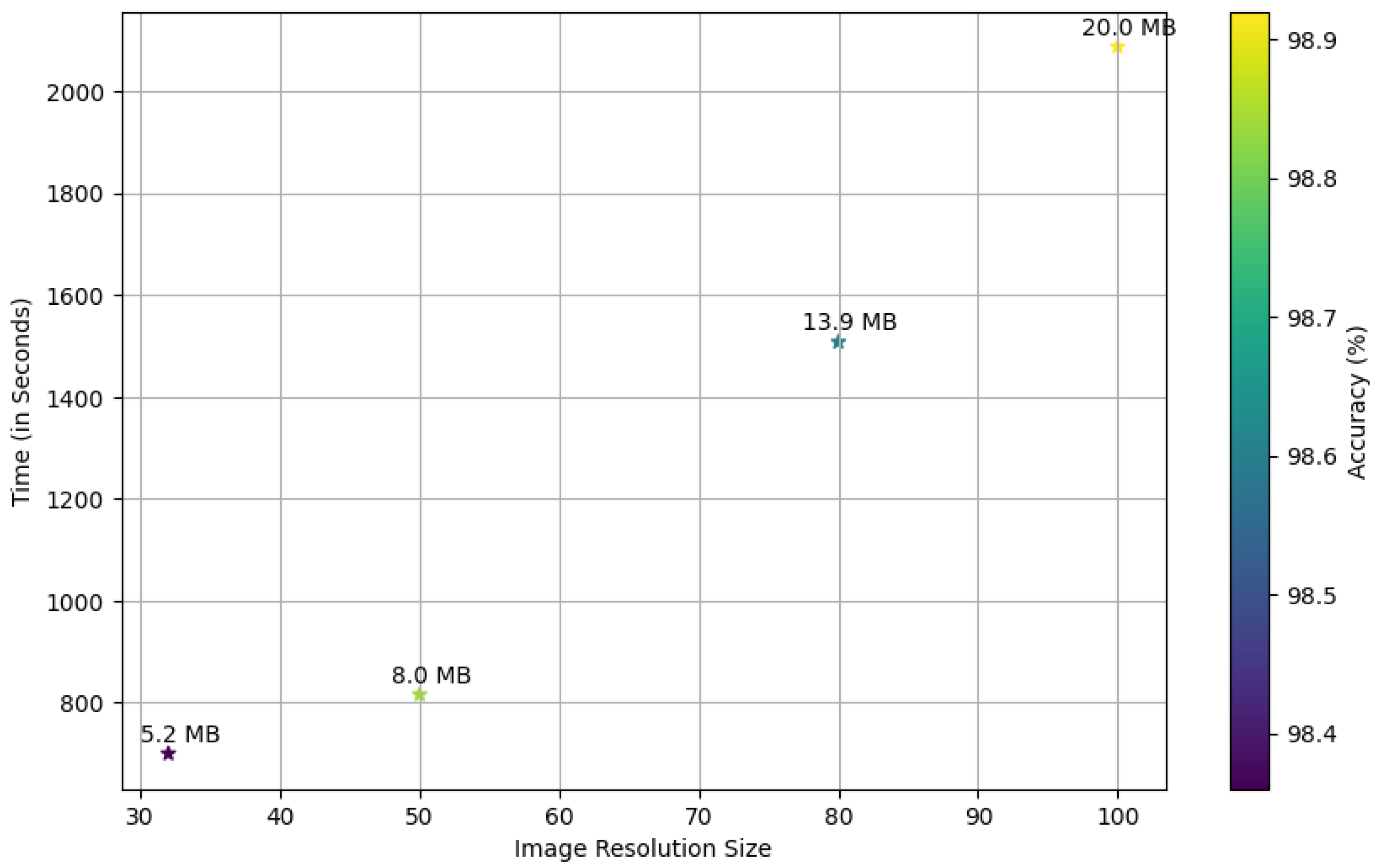
In this study, we conducted a comprehensive analysis using a selected subset of the German Traffic Sign Recognition Benchmark (GTSRB) dataset to examine the impact of image resolution variations on the performance of our traffic sign classification model. The primary objective was to discern the effect of different image sizes on the model’s capability in accurately classifying traffic signs. This process entailed a systematic evaluation of the model using a range of image resolutions, specifically, 32 × 32, 50 × 50, 80 × 80, and 100 × 100 pixels. The intent was to establish an optimal balance between computational complexity and the efficiency of classification performance, as depicted in Figure 1.

After careful consideration, we excluded higher image resolutions of 150 × 150 and 200 × 200 pixels due to their high computational requirements, which exceeded 3000 s.

After thoroughly analyzing these factors, we opted for a 50 × 50 pixel image resolution, finding it to be an optimal balance between classification accuracy and the complexity of the model. Our experimentation showed that (as shown in

Table 4. Comparative analysis of TSR performance on GTSRB.

Image Resolution Size	Time (in Seconds)	Resources Usage (in MByte)	Accuracy (%)	F1-Score (%)
32 × 32	700.2	5.2	98.36	98.33
50 × 50	816.1	8.0	98.84	98.40
80 × 80	1507.6	13.9	98.60	98.59
100 × 100	2086.8	20.0	98.92	98.64

) lower resolution images led to a notable decrease in the model’s classification accuracy. Meanwhile, high resolution images led to an increase in the model’s complexity and longer training times.

The primary goals regarding image size focused on attaining high accuracy while concurrently reducing training durations and resource consumption. After careful deliberation, including examining the accuracy–computational efficiency trade-off, we concluded that employing 50 × 50 pixel images represented the optimal choice for our proposed TSR system. Moreover, the proposed model is designed for real-world implementation in safety-critical scenarios, where accuracy and reliability are of utmost importance. We contend that using higher resolution images leads to more accurate detection and classification of traffic signs, a crucial factor in ensuring the safety of drivers and pedestrians. Consequently, we proceeded to train and evaluate our proposed model on the GTSRB, ITSD, and BTSD datasets to thoroughly assess its efficacy and reliability in the context of TSR. During the training process, we employed the Adam optimizer with a learning rate of 0.01.

Furthermore, we integrated various data enhancement techniques, such as random rotations, zooming, and horizontal flips, to increase the training set and enhance the generalization capabilities of the model. Our experiments were executed on a Jupyter Notebook environment powered by a GeForce RTX 2080 Ti GPU. The primary implementation was accomplished using Python 3.8.

4.2. Evaluation Parameters

The performance of classification models, like our proposed traffic sign recognition model, is often gauged using key performance indicators (KPIs) such as accuracy, precision, recall, and the F1-score.

Accuracy ($\mathbb{A}$) is a fundamental KPI that denotes the overall accuracy of the model’s predictions. It is determined by the ratio of accurately classified instances relative to the total count of instances, as depicted in Equation (5). Accuracy provides a holistic view of the model’s performance, giving an overall success rate of classification.

$$\mathbb{A}=\frac{T_P+T_N}{T_P+T_N+F_P+F_N}$$

(5)

Precision ($\mathbb{P}$) is calculated as the ratio of true positives $T_P$ (i.e., correct positive predictions) to all the positive predictions made by the model, calculated in Equation (6). Precision gives us an understanding of the model’s ability to avoid false positives $F_P$, thus ensuring that the detected traffic signs are indeed correct.

$$\mathbb{P}=\frac{T_P}{T_P+F_P}$$

(6)

Recall ($\mathbb{R}$), also known as sensitivity, gauges the model’s completeness. It measures the percentage of true positives out of all the actual positive cases present in the dataset, as outlined in Equation (7). Recall gives insight into the model’s ability to correctly identify all relevant instances, thus helping avoid false negatives $F_N$, which, in the context of traffic sign recognition, means missing actual traffic signs.

$$\mathbb{R}=\frac{T_P}{T_P+F_N}$$

(7)

The F1-score ($\mathbb{F}1-\mathrm{score}$) represents the harmonic mean of precision and recall, according to Equation (8). This KPI provides a balanced perspective by considering both precision and recall, thus presenting a more comprehensive view of the model’s performance. A high F1-score indicates that the model has a robust performance with a balance between precision and recall.

$$\mathbb{F}1-\mathrm{score}=2\times \frac{\mathbb{P}\times \mathbb{R}}{\mathbb{P}+\mathbb{R}}$$

(8)

In our experiments, we rely on these KPIs as the key metrics for evaluating our proposed model’s performance. They provide us comprehensive insights into the proposed model while maintaining a balance between detecting all relevant signs and avoiding false detections.

4.3. Performance Results: GTSRB Dataset [29]

We conducted extensive experiments using the GTSRB dataset to comprehensively assess the effectiveness and reliability of our proposed model for TSR. GTSRB is widely recognized and serves as a benchmark for evaluating the TSR framework. To establish a solid comparison, we compared the performance of our proposed model with several state-of-the-art frameworks (SOTA), such as VGG19 [33], VGG16 [33], ResNet50V2 [34], MobileNetV2 [35], DenseNet121 [36], DenseNet201 [36], NASNetMobile [37], and EfficientNet [38].

The experimental results, as shown in

Table 5. Comparative performance analysis of TSR on the GTSRB dataset.

Method	Accuracy (%)	Precision (%)	Recall (%)	F1-Score (%)	Training Time (in Seconds)	Response Time (in Milliseconds)	Resources Usage (in MByte)
VGG19 [33]	98.17	98.29	98.17	98.16	1418.0	103.96	15.2
VGG16 [33]	98.39	98.47	98.39	98.29	1176.5	97.41	16.7
ResNet50V2 [34]	95.82	95.96	95.82	95.76	2434.0	174.37	8.4
MobileNetV2 [35]	94.99	95.57	94.99	95.07	1934.6	131.96	10.0
DenseNet121 [36]	98.56	98.63	98.56	98.56	3437.8	232.20	11.6
DenseNet201 [36]	98.81	98.83	98.81	98.80	5081.0	289.43	11.6
NASNetMobile [37]	97.33	97.39	97.33	97.31	4590.2	210.70	11.6
EfficientNet [38]	97.64	97.68	97.64	97.62	2303.8	165.74	12.8
Ours	98.85	98.91	98.85	98.84	840.9	96.95	14.0

, clearly demonstrate that the proposed model outperforms the SOTA frameworks, such as VGG19, VGG16, ResNet50V2, MobileNetV2, DenseNet121, DenseNet201, NASNetMobile, and EfficientNet, in accurately classifying traffic signs. The proposed model achieved an accuracy of 98.85%, outperforming the other SOTA frameworks by 0.68%, 0.46%, 3.03%, 3.86%, 0.29%, 0.04%, 1.52%, and 1.21%, respectively. These results highlight the effectiveness of our model in achieving highly accurate predictions, while, in terms of precision, the proposed model achieves a precision score of 98.91%, outperforming VGG19 with a precision score of 98.29%, VGG16 with 98.47%, ResNet50V2 with 95.96%, MobileNetV2 with 95.57%, DenseNet121 with 98.63%, DenseNet201 with 98.83%, NASNetMobile with 97.39%, and EfficientNet with 97.68%. The proposed model outperforms these state-of-the-art frameworks with percentage differences ranging from 0.29% to 1.62%. This higher precision score highlights the robustness and ability of the proposed model to minimize false positives and accurately identify positive instances of traffic signs. The improved precision further reinforces the effectiveness and reliability of our model in the classification of traffic signs.

Furthermore, our proposed model exhibited a recall performance, achieving a recall score of 98.85%, outperforming VGG19, VGG16, ResNet50V2, MobileNetV2, DenseNet121, DenseNet201, NASNetMobile, and EfficientNet with a recall score of 98.17%, 98.39%, 95.82%, 95.82%, 98.56%, 98.81%, 97.33%, 97.64%, respectively. Compared to these SOTA frameworks, the proposed model outperforms these models with a percentage difference of 0.68%, 0.46%, 3.03%, 3.86%, 0.29%, 0.04%, 1.52%, and 1.21%.

In evaluating overall balanced performance, we considered the F1-score metric, which provides a comprehensive assessment, taking into account both precision and recall. Our model achieved an F1 score of 98.84%, outperforms VGG19 with 98.16%, VGG16 with 98.29%, ResNet50V2 with 95.76%, MobileNetV2 with 95.07%, DenseNet121 with 98.56%, DenseNet201 with 98.80%, NASNetMobile with 97.31%, and EfficientNet with 97.62%. The percentage differences between our model and these SOTA frameworks range from 0.68% to 3.82%. These findings emphasize the remarkable balance our model strikes between precision and recall, solidifying its reliability and excellence in tackling traffic sign recognition tasks. 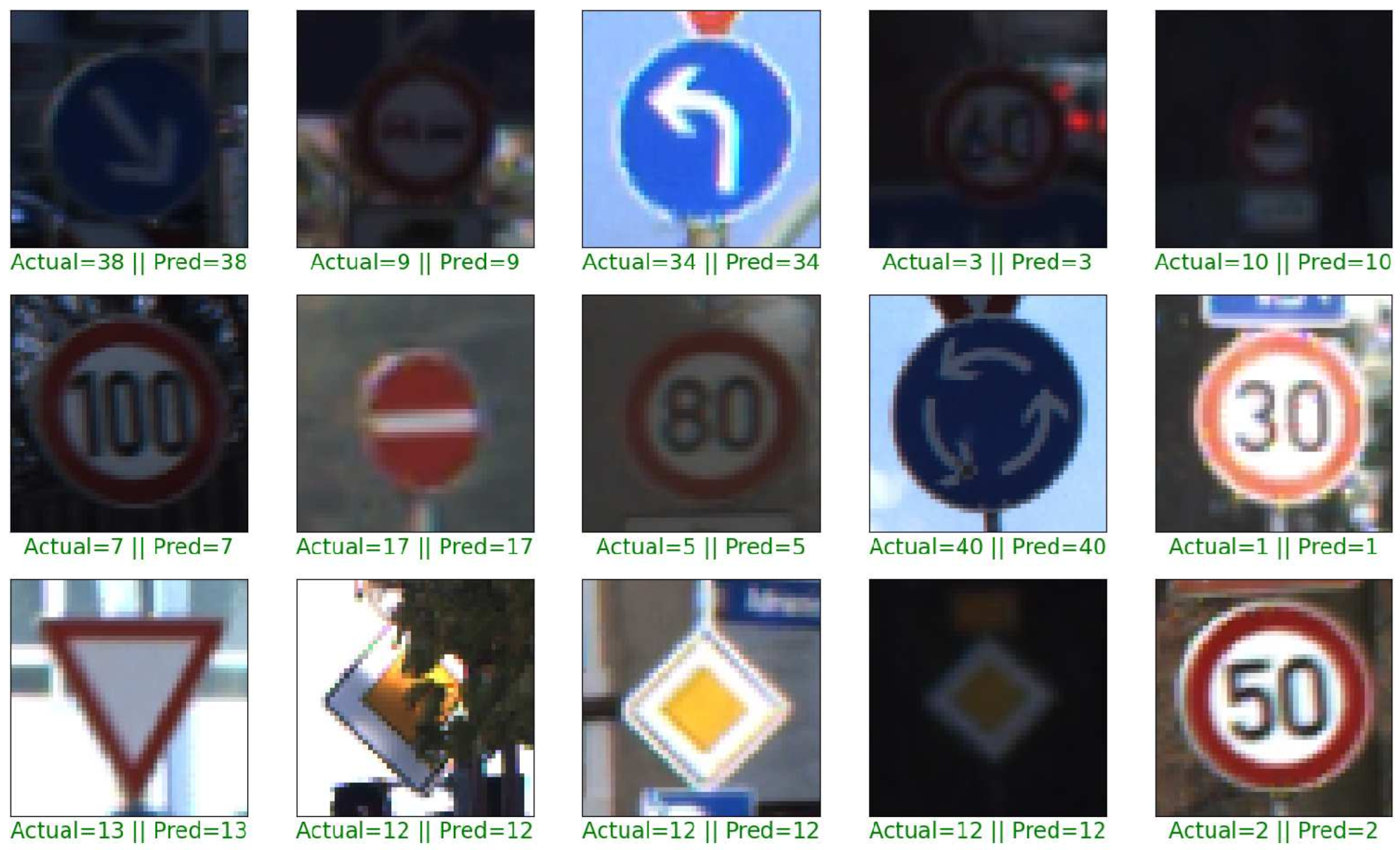Figure 2 provides visual evidence of the positive instance capture rates achieved by our proposed model, highlighting its exceptional performance in accurately classifying traffic signs.

In addition to excellent classification performance, our proposed model exhibited notable computational efficiency. It achieved a training time of 840.9 s, which is significantly faster compared to VGG19, VGG16, ResNet50V2, MobileNetV2, DenseNet121, DenseNet201, NASNetMobile, and EfficientNet, with percentage improvements ranging from 28.4% to 83.5%. Similarly, the proposed model demonstrated faster response times, with a response time of 96.95 milliseconds, outperforming competing methods by 6.7% to 63.3%. These results highlight the efficiency of the model in training, real-time processing of traffic signs, and make it suitable for real-world scenarios, where accurate and efficient traffic sign classification is of paramount importance to ensure road safety and enable ITS.

4.4. Performance Results: ITSD Dataset [30]

To further validate the performance of the proposed model, we evaluated the proposed model on the ITSD dataset. The proposed model achieves an accuracy of 92.41%, outperforming VGG19, VGG16, ResNet50V2, MobileNetV2, DenseNet121, DenseNet201, NASNetMobile, and EfficientNet, with an accuracy of 85.25%, 90.76%, 89.76%, 88.54%, 92.26%, 92.26%, 88.83%, and 90.40%, respectively (as shown in

Table 6. Comparative performance analysis of TSR on the ITSD dataset.

Method	Accuracy (%)	Precision (%)	Recall (%)	F1-Score (%)	Training Time (in Seconds)	Response Time (in Millisecond)	Resources Usage (in MByte)
VGG19 [33]	85.25	84.61	85.25	83.99	483.0	89.42	5.6
VGG16 [33]	90.76	91.76	90.76	90.96	405.5	97.41	5.9
ResNet50V2 [34]	89.76	90.77	89.76	90.01	826.0	172.03	4.9
MobileNetV2 [35]	88.54	89.26	88.54	87.48	672.7	131.74	5.2
DenseNet121 [36]	92.26	93.07	92.26	92.44	1165.6	190.25	6.2
DenseNet201 [36]	92.26	93.19	92.26	92.45	1710.9	329.96	6.2
NASNetMobile [37]	88.83	89.90	88.83	88.93	1544.1	211.33	7.0
EfficientNet [38]	90.40	90.44	90.40	89.24	753.3	170.00	7.1
Ours	92.41	93.37	92.41	92.62	283.3	78.56	6.7

). It is important to note that the proposed model shows an improvement of 7.16% compared to VGG19 and other models, with percentage differences ranging from 0.17% to 4.24%. These results underscore the superior ability of our proposed model to accurately classify traffic signs.

Furthermore, in terms of precision, the proposed model achieves a precision score of 93.37%, outperforming VGG19, VGG16, ResNet50V2, MobileNetV2, DenseNet121, DenseNet201, NASNetMobile, and EfficientNet, with precision scores of 84. 61%, 91.76%, 90.77%, 89.26%, 93.07%, 93.19%, 89.90%, and 90.44%, respectively. These results (as shown in Table 6) highlight the ability of the proposed model to minimize false positives and accurately identify positive instances of traffic signs.

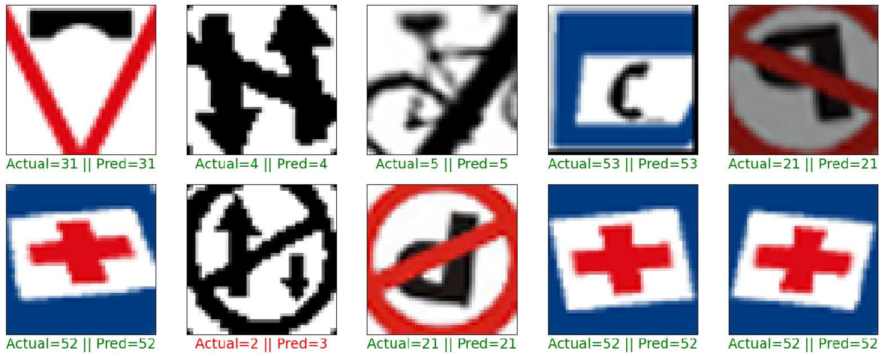
In terms of recall, the proposed model achieves a score of 92.41%, outperforming VGG19, VGG16, ResNet50V2, MobileNetV2, NASNetMobile, and EfficientNet by 8.63% 1.66%, 2.61%, 5.14% 3.69%, and 3.38%, respectively. Similarly, Figure 3 provides a comprehensive performance visualization of the proposed model in accurately capturing positive instances of traffic signs. Additionally, the proposed model excels in the F1-score, achieving a score of 92.62%, outperforming VGG19, VGG16, ResNet50V2, MobileNetV2, DenseNet121, DenseNet201, NASNetMobile, and EfficientNet, with percentage differences ranging from 0.17% to 10.20%.

In addition to exceptional classification performance, the proposed model also shows its efficiency by achieving a training time of 283.3 s, which is approximately 41.3%, 30.4%, 65.7%, 57.7%, 75.7%, 83.4%, 81.6%, and 64.5% faster compared to VGG19, VGG16, ResNet50V2, MobileNetV2, DenseNet121, DenseNet201, NASNetMobile, and EfficientNet, respectively. Similarly, in terms of response time, the proposed model excels with a response time of 78.56 milliseconds, which is approximately 12.2%, 19.4%, 54.4%, 40.3%, 58.8%, 65.2%, 62.8%, and 53.8% faster compared to VGG19, VGG16, ResNet50V2, MobileNetV2, DenseNet121, DenseNet201, NASNetMobile, and EfficientNet, respectively.

In conclusion, the proposed model demonstrates superior performance in multiple aspects compared to VGG19, VGG16, ResNet50V2, MobileNetV2, DenseNet121, DenseNet201, NASNetMobile, and EfficientNet. It achieves a higher accuracy, precision, recall, and F1-score, with notable percentage differences ranging from 0.17% to 10.20%. Moreover, the proposed model stands out with its faster training and response times, while maintaining a balance between runtime and memory consumption. This efficiency makes it highly effective for TSR and ITS. With faster learning from the dataset and efficient processing of traffic signs, the proposed model excels in real-time applications. These advantages highlight its efficacy in efficiently performing TSR tasks, contributing to improved road safety and advanced ITS.

4.5. Performance Results: BTSD Dataset [31]

Table 7. Comparative performance analysis of TSR on the BTSD dataset.

Method	Accuracy (%)	Precision (%)	Recall (%)	F1-Score (%)	Training Time (in Seconds)	Response Time (in Millisecond)	Resources Usage (in MByte)
VGG19 [33]	42.89	37.09	42.89	36.67	351.6	116.31	6.1
VGG16 [33]	73.92	79.71	73.92	72.75	297.1	108.46	6.5
ResNet50V2 [34]	10.43	21.30	10.43	7.52	349.2	144.29	6.6
MobileNetV2 [35]	9.32	41.32	9.32	8.79	273.3	126.82	6.8
DenseNet121 [36]	8.88	11.79	8.88	4.59	474.8	190.35	7.1
DenseNet201 [36]	8.45	16.24	8.45	8.98	682.5	237.49	7.6
NASNetMobile [37]	0.75	0.33	0.75	0.35	635.8	208.11	8.4
EfficientNet [38]	2.38	6.24	2.38	2.27	326.5	169.63	8.9
Ours	92.69	95.05	92.26	93.35	248.9	95.67	9.6

presents the results of the comparative performance analysis of TSR on the BTSD dataset. Our proposed model achieved an accuracy of 92.26%, outperforming VGG19, VGG16, ResNet50V2, MobileNetV2, DenseNet121, DenseNet201, NASNetMobile, and EfficientNet, with accuracy scores of 42.89%, 73.92%, 10.43%, 9.32%, 8.88%, 8.45%, 0.75%, and 2.38%, respectively. These results highlight substantial performance differences between the proposed and SOAT frameworks, demonstrating the superior classification capability of our model on the BTSD dataset.

Precision, a crucial metric to minimize false positives, was also significantly higher for our proposed model, achieving a precision score of 93.64%, compared to VGG19, VGG16, ResNet50V2, MobileNetV2, DenseNet121, DenseNet201, NASNetMobile, and EfficientNet precision scores of 37.09%, 79.71%, 21.30%, 41.32%, 11.79%, 16.24%, 0.33%, and 6.24%, respectively. These results underscore the effectiveness of our model in accurately identifying positive instances of traffic signs. Furthermore, compared to these SOTA frameworks, our model outperformed VGG19, VGG16, ResNet50V2, MobileNetV2, DenseNet121, DenseNet201, NASNetMobile, and EfficientNet by percentage differences of 51.37%, 18.68%, 18.68%, 88.49%, 83.90%, 91.67%, 83.90%, and 68.49%, respectively.

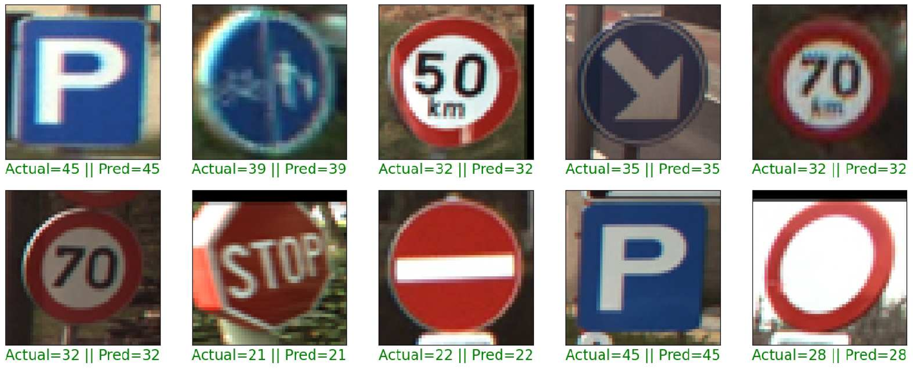
The F1-score, a balanced measure of precision and recall, further reinforces the strength of our model, achieving an impressive F1-score of 92.01%. Our proposed model outperformed VGG19, VGG16, ResNet50V2, MobileNetV2, DenseNet121, DenseNet201, NASNetMobile, and EfficientNet by percentage differences of 1.66%, 19.59%, 15.35%, 45.34%, 60.96%, 83.54%, 17.46%, and 4.20%, respectively. In addition to accuracy, precision, recall, and F1-score, our proposed model exhibited efficient computational performance. It achieved a training time of 248.9 s, outperforming VGG19, VGG16, ResNet50V2, MobileNetV2, DenseNet121, DenseNet201, NASNetMobile, and EfficientNet by percentage differences of 29.6%, 9.6%, 28.7%, 28.2%, 53.6%, 67.6%, 28.8%, and 57.4%, respectively (as shown in Figure 4).

Our model also demonstrated faster response times, with a response time of 95.67 milliseconds, outperforming VGG19, VGG16, ResNet50V2, MobileNetV2, DenseNet121, DenseNet201, NASNetMobile, and EfficientNet by percentage differences of 13.8%, 26.5%, 39.2%, 29.3%, 44.2%, 58.0%, 49.4%, and 46.4%, respectively. These findings showcase the efficiency of the model in real-time traffic sign processing on the BTSD dataset.

By outperforming state-of-the-art methods in terms of accuracy, precision, recall, F1-score, and computational efficiency, our model demonstrates its potential for real-time traffic sign processing and classification. Our proposed CNN-based model for TSR tasks has been demonstrated to have exceptional classification performance, efficient computational performance, and significant improvements over other methods, thus confirming its robustness and effectiveness.

4.6. Feature Visualization and Interpretation

To make our model interpretable and transparent, we employ several explainability techniques, including LIME (Local Interpretable Model-Agnostic Explanations) and Grad-CAM (Gradient-weighted Class Activation Mapping), to understand how the model arrives at its predictions. Furthermore, these state-of-the-art techniques enable us to visualize and highlight the regions of input images that have the most significant influence on the model’s predictions.

LIME is a technique that provides explanations for individual predictions by approximating the behavior of the model locally. It approximates the behavior of the model around a specific input by creating perturbations and observing the response of the model. To gain insight into the proposed model, we implemented LIME to identify the pixel intensities and patterns that contribute to the model decision-making process. By sampling multiple perturbed versions of the input image and measuring the model prediction changes, the most influential features or regions of the input are identified for GTSRB, ITSD, and BTSD. This comparative analysis is visually represented in Figure 5, where each figure contains three graphs representing these scenarios. These graphs illustrate how different features or regions influence model predictions between scenarios, providing a clear and comprehensive visual representation of the proposed model behavior under varying conditions.

Furthermore, Grad-CAM highlights the relevant regions of an input image that contribute to the model’s prediction. By computing the gradients of the target class with respect to the model’s convolutional feature maps, Grad-CAM generates a heat map visualization of the regions where the model focuses its attention for decision making. We employed Grad-CAM to gain insight, identify, and view the salient features (as shown in Figure 6) that are contributing to the proposed model’s prediction. Analyzing these highlighted regions allows us to gain valuable insights into the image regions the model considers crucial for accurate TSR decisions.

By leveraging LIME and Grad-CAM techniques, we gain insights into the decision-making process of our model and gain a better understanding of the features and regions that are significant in making accurate traffic sign predictions and are able to obtain a comparative view of its performance across different scenarios. This comparative approach (as illustrated in Figure 5 and Figure 6) provides us with a clear comparison across the datasets, enhances our understanding of the features and regions significant in making accurate traffic sign predictions, and further explains the proposed model predictions, thereby enhancing the transparency and interpretability of our proposed CNN-based model.

5. Discussion

The results of the evaluation of the proposed model in three diverse datasets provide crucial insights into the capabilities of the proposed model. In this comprehensive discussion, we delve into the findings in detail and explore their implications and real-world applications.

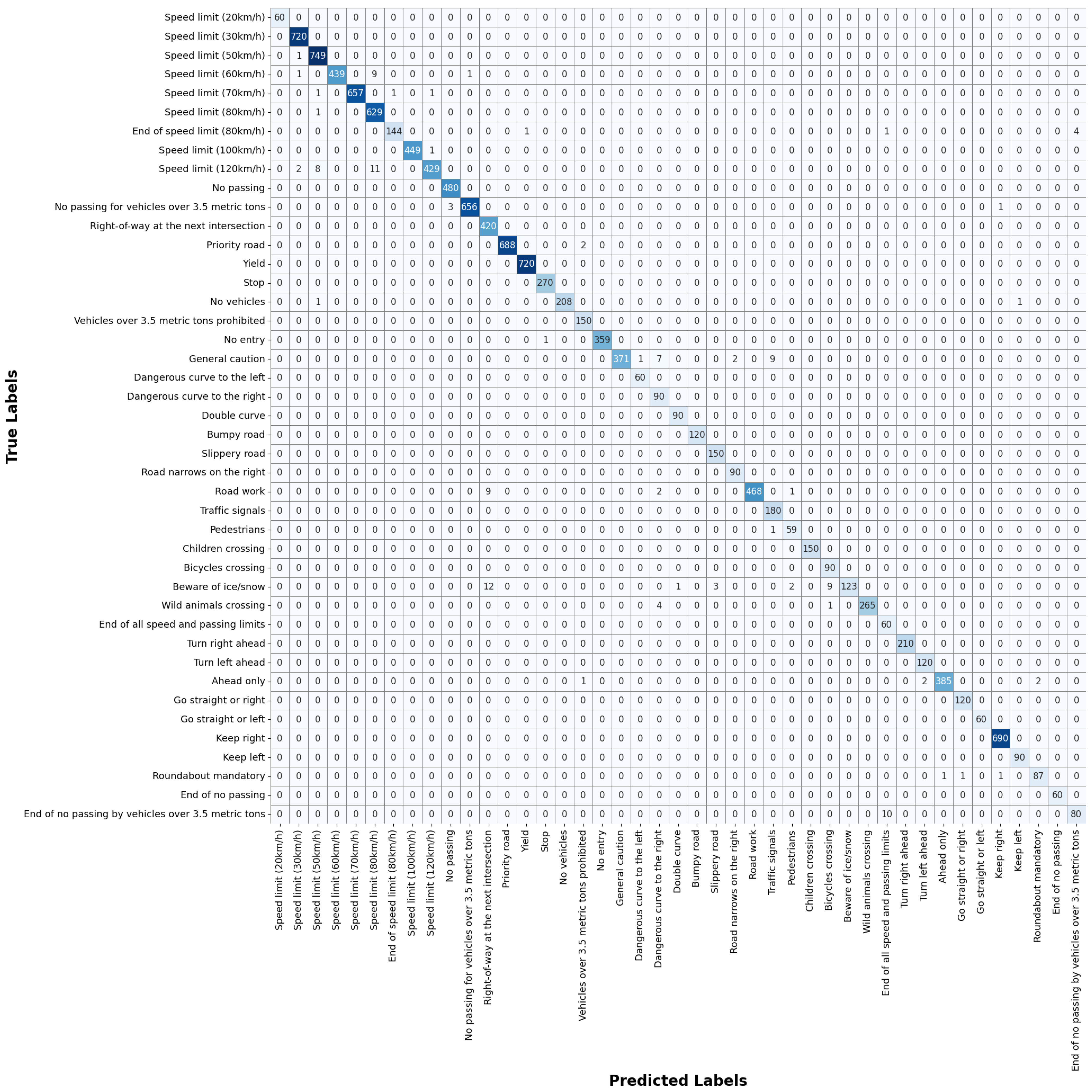
The proposed model accuracy across GTSRB, ITSD, and BTSD datasets demonstrates its generalization capabilities, making it suitable for real-world implementation. By correctly classifying the traffic signs, the proposed model exhibits its efficiency and reliability of traffic management in ITS. Appendix A presents the confusion matrix of the proposed model for the GTSRB, providing a breakdown of the predicted labels against the ground truth labels. 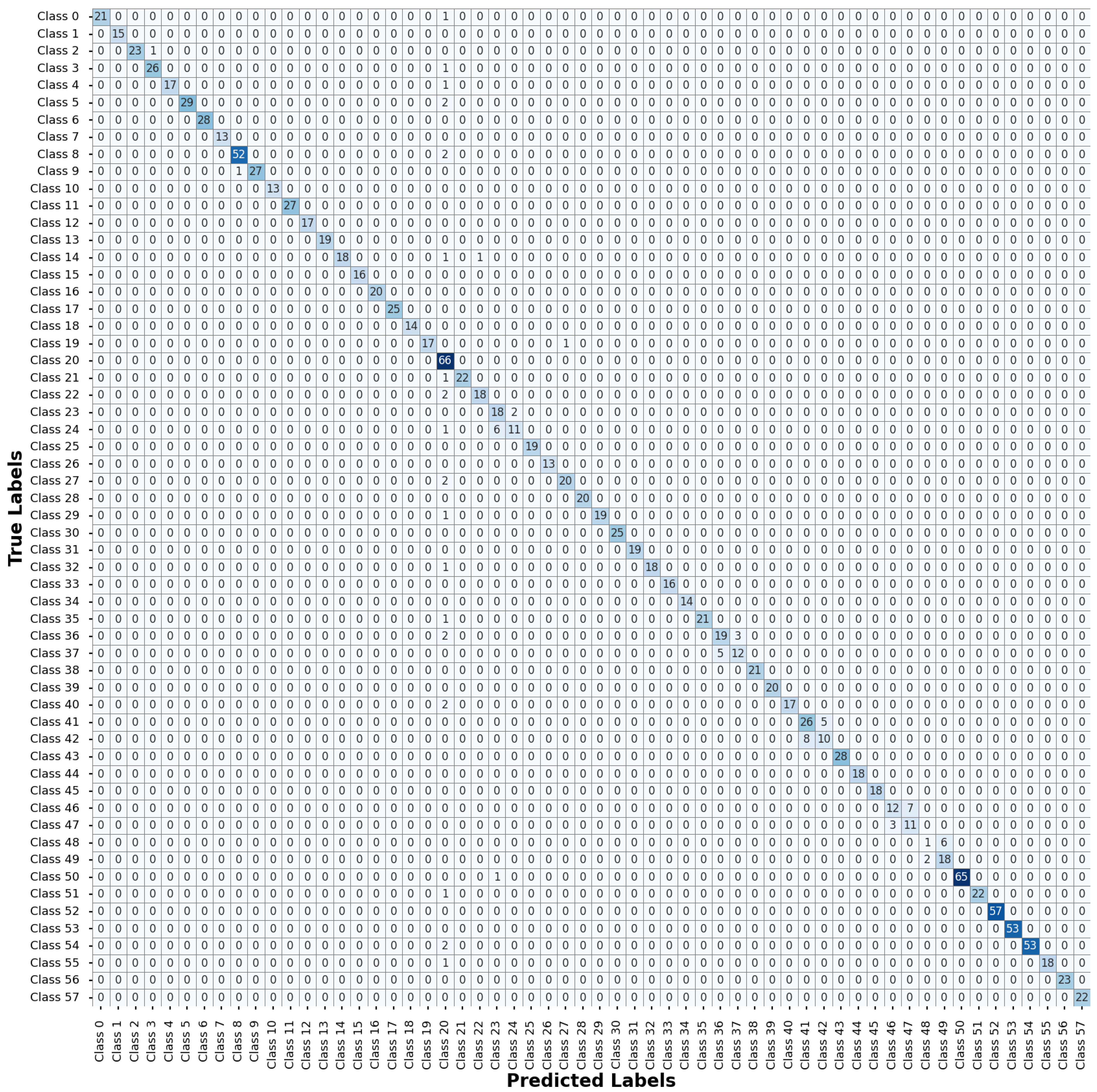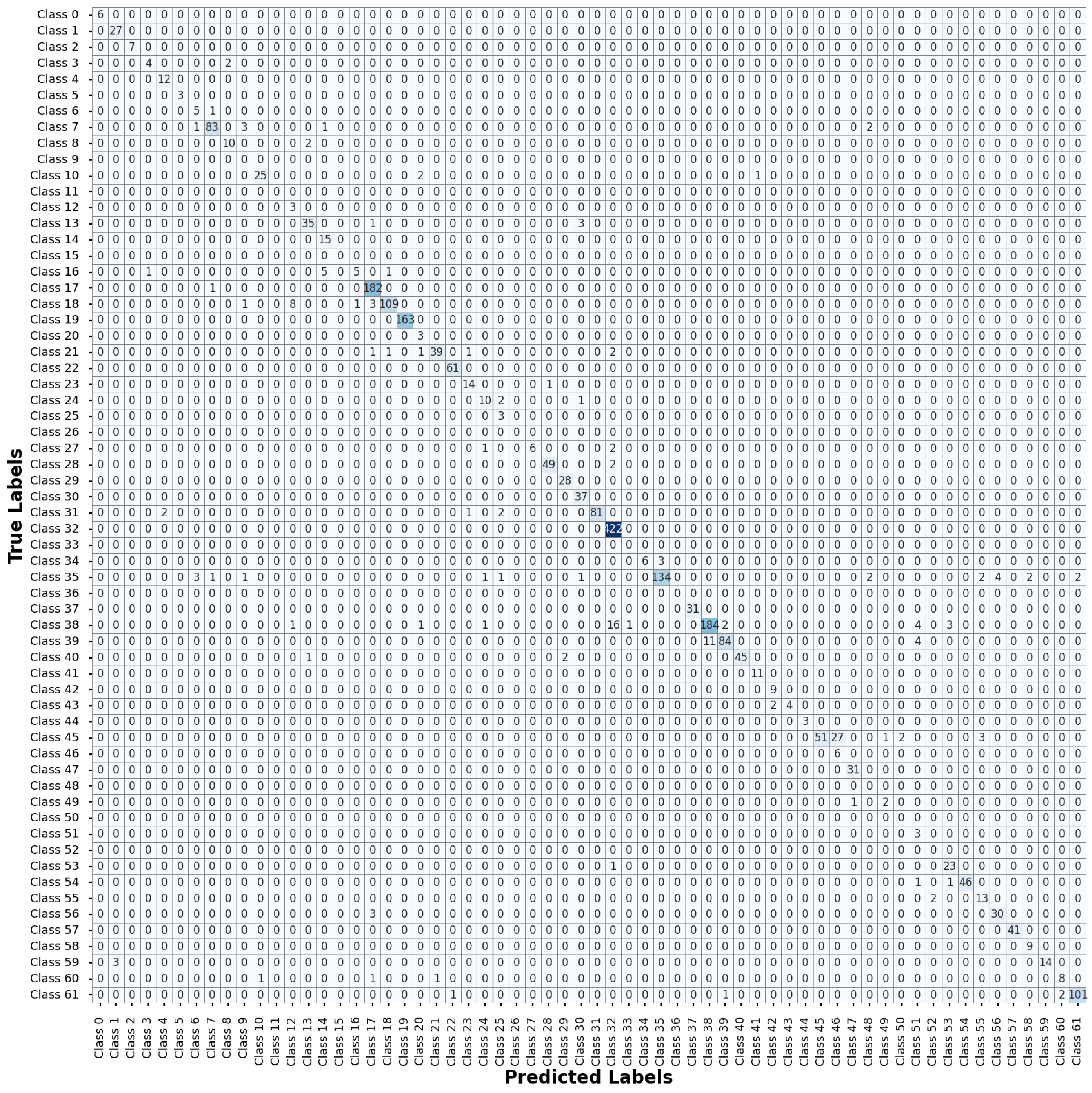Similarly, Appendix B and Appendix C present the confusion matrix for ITSD and BTSD, respectively. These matrices provide a granular representation of the classification results, facilitating a thorough evaluation of the accuracy and performance characteristics of the proposed model. By analyzing these matrices, we can identify specific classes where the models excel or struggle, providing valuable insights into their strengths and areas for potential enhancement.

A high recall score indicates the potential of the proposed model to correctly identify the actual traffic signs present in the scenes, thereby minimizing false negatives. In real-world scenarios, missing or misclassifying a traffic sign can have severe safety implications, especially in autonomous vehicle systems. Meanwhile, F1-scores obtained from all three datasets provide insight into the proposed model balance between precision and recall. Maintaining this balance is crucial, as both false positives and false negatives can have serious consequences for traffic safety and efficiency. Traffic sign designs, weather conditions, and lighting can vary considerably between different regions. Therefore, the high recall and F1-score of our model underscores its effectiveness in promoting road safety and ensuring accurate TSR.

In our study, we integrated Explainable AI (XAI) techniques, specifically LIME and Grad-CAM, to enhance the performance of our traffic sign recognition model. These techniques have proven instrumental not only in providing interpretability, but also in substantially improving the accuracy, reliability, and generalization capabilities of the proposed model. By employing LIME, we have been able to dissect and understand the salient features in traffic sign images that are prioritized by our model, as shown in Figure 5. These insights have been the key to improving our model to identify pertinent attributes and features, leading to a more accurate classification. In particular, we observed that our model focused on distinct shapes and colors pertinent to traffic signs, allowing us to fine-tune the feature extraction layers to improve detection and classification accuracy. Grad-CAM has been a crucial tool in providing visual explanations through heat maps, as illustrated in Figure 6. These heat maps highlight areas within the images that are integral to the proposed model decision-making process. These insights have been critical for optimizing the convolutional layers within our model. Concentrating on salient patterns and textures has significantly improved the model reliability and robustness, especially under challenging conditions, such as variable lighting, sign occlusion, and scenarios involving partially visible signs.

In real-world applications, the increased interpretability and transparency provided by these XAI techniques are invaluable. This helps to build between users and stakeholders by making the decision-making process more transparent and simplifying the identification and correction of errors. This aspect is particularly crucial in dynamic and diverse traffic environments, where the accuracy of traffic sign recognition directly impacts safety and efficiency. For autonomous vehicles operating in diverse real-world conditions, the ability of the model to accurately interpret traffic signs is paramount. Misinterpretation or failure to recognize traffic signs can lead to serious safety implications [39,40,41]. The insights provided by LIME and Grad-CAM are particularly valuable in these scenarios. They ensure that the model not only performs with high accuracy, but also demonstrates robustness and adaptability to the complexities and variabilities of different road and weather conditions. Therefore, by employing these XAI techniques, the safety and efficiency of autonomous transportation systems are significantly improved by enhancing the ability of the model to recognize traffic signs accurately and reliably.

Although our proposed model exhibits impressive performance, it is essential to acknowledge potential limitations. The proposed model demonstrates good generalizability across the three datasets; however, further investigation is necessary to evaluate its performance on additional datasets from different regions and under various conditions. Furthermore, the computational resources required to train and implement the proposed model could be a challenge for real-time applications on edge devices. Striking a balance between accuracy and computational efficiency will be crucial for practical deployment.

6. Conclusions

In this paper, we present an interpretable, robust, and computationally efficient neural network-based model for traffic sign recognition (TSR), achieving an accuracy rate of 98.85% on the German Traffic Sign Recognition Benchmark (GTSRB), 94.73% on the Indian Traffic Sign Dataset (ITSD), and 92.26% on the Belgian Traffic Sign Dataset (BTSD). Our model outperforms several state-of-the-art frameworks, including DenseNe, NASNetMobile, EfficientNet, and others in key metrics such as precision, recall, and F1-score. Its notable computational efficiency, characterized by reduced training and inference times, combined with its ability to handle diverse traffic signs and adapt to various environmental conditions, makes it well-suited for real-time applications in Intelligent Transportation Systems (ITS), where rapid decision-making is critical. The incorporation of Explainable AI (XAI) techniques, such as Local Interpretable Model-Agnostic Explanations (LIME) and Gradient-weighted Class Activation Mapping (Grad-CAM), significantly enhances the transparency and interpretability of the model, providing deeper insights into its decision-making process. In the future, we will focus on further refining the interpretability features of the model by exploring Brain-inspired Modular Training for enhanced XAI capabilities and considering the integration of Large Language Models (LLM). Additionally, we aim to investigate how Visual Language Models (VLMs) and LLMs can be effectively combined to provide richer, context-aware explanations, improving the model performance and reliability in real-world traffic scenarios.