

Comparison of a Hybrid Firefly–Particle Swarm Optimization Algorithm with Six Hybrid Firefly–Differential Evolution Algorithms and an Effective Cost-Saving Allocation Method for Ridesharing Recommendation Systems

Abstract
:1. Introduction
2. Optimization Problem in Ridesharing Recommendation Systems and a New Proportional Method to Allocate Cost Savings
3. Development of Hybrid Algorithms Based on Hybridization of Firefly Algorithm with PSO or DE
| Procedure 1: CS to map a real value to zero or one |
| Input: Output: Begin If If Generate return End |
3.1. Fitness Function
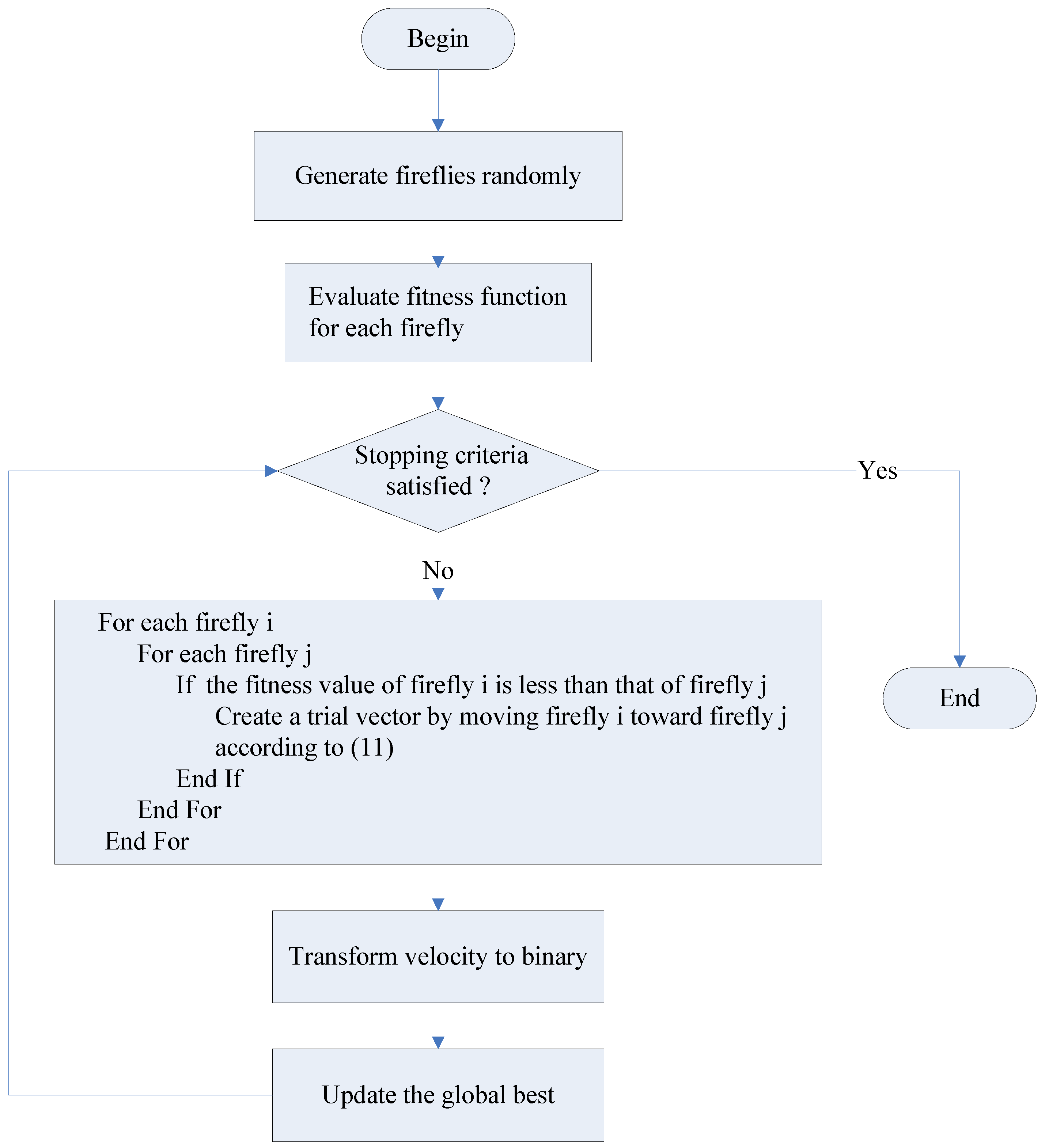
3.2. Firefly Algorithm
| Algorithm 1: Discrete Firefly Algorithm |
| Input: , Output: the global best, Step 1: Generate fireflies in the initial population of swarm Step 2: While () Evaluate the fitness function for For each For each If For Move the i-th firefly toward the j-th firefly in the n-th dimension: Transform to binary and update i-th firefly i as follows: Generate randomly based on uniform distribution End For Evaluate End If End For End For Update the global best End While |
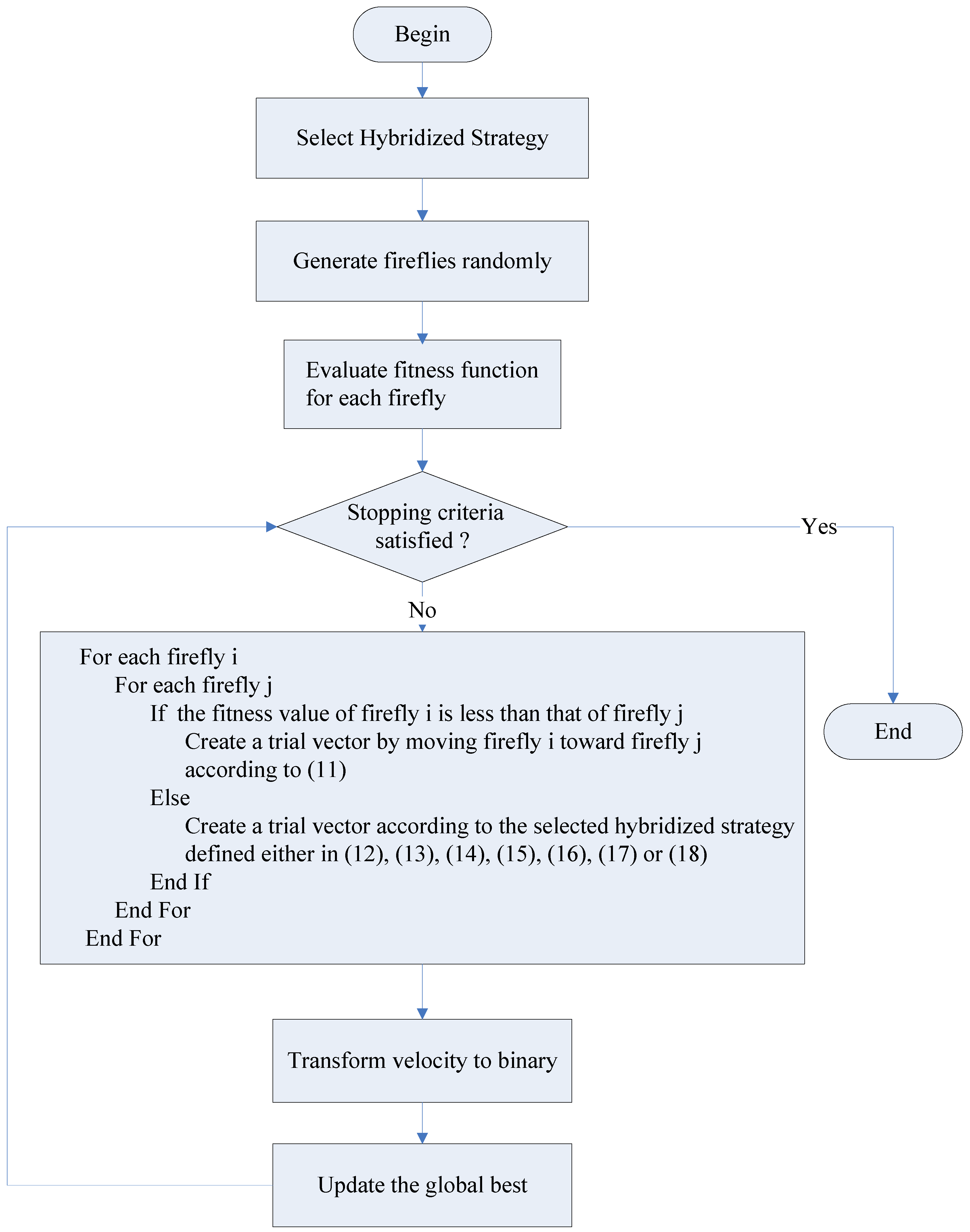
3.3. Discrete Firefly-PSO (FPSO) Algorithm and Discrete Firefly-DEi (FDEi) Algorithm
| Algorithm 2: Discrete Firefly-PSO (FPSO) Algorithm |
| Input: , Output: the global best, Step 1: Generate fireflies in the initial population of swarm Step 2: While () Evaluate the fitness function for each firefly For each For each If Step 2.1: Fly according to fireflies’ pattern For Move the i-th firefly toward the j-th firefly in the n-th dimension Transform to binary and update -th firefly as follows: Generate randomly based on uniform distribution End For Else Step 2.2: Fly according to particle swarm’s pattern to attempt to increase diversity For Generate , a random variable with uniform distribution Generate , a random variable with uniform distribution Transform each element of the trial vector to one or zero End For End If End For End For Update the global best End While |
| Algorithm 3: Discrete Firefly-DEi (FDEi) Algorithm |
| Input: , Output: the global best, Step 1: Generate fireflies in the initial population of swarm Step 2: While () Evaluate the fitness function for each firefly For each For each If Step 2.1: Fly according to fireflies’ pattern For Move the i-th firefly toward the j-th firefly in the n-th dimension Transform as follows: Generate randomly based on uniform distribution End For Else Step 2.2: Fly according to particle swarm’s pattern to attempt to increase diversity For Apply Strategy DEi to create the n-th dimension of trial vector Transform each element of the trial vector to one or zero End For End If End For End For Update the global best End While |
4. Results
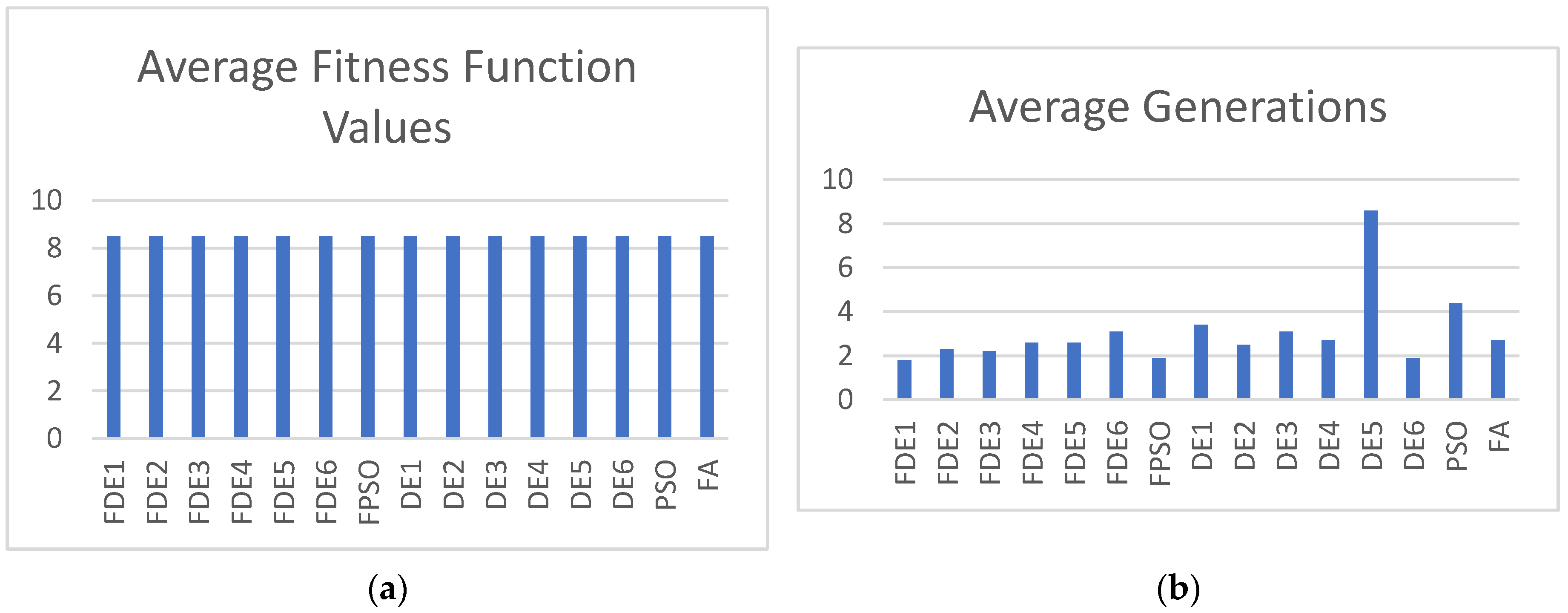
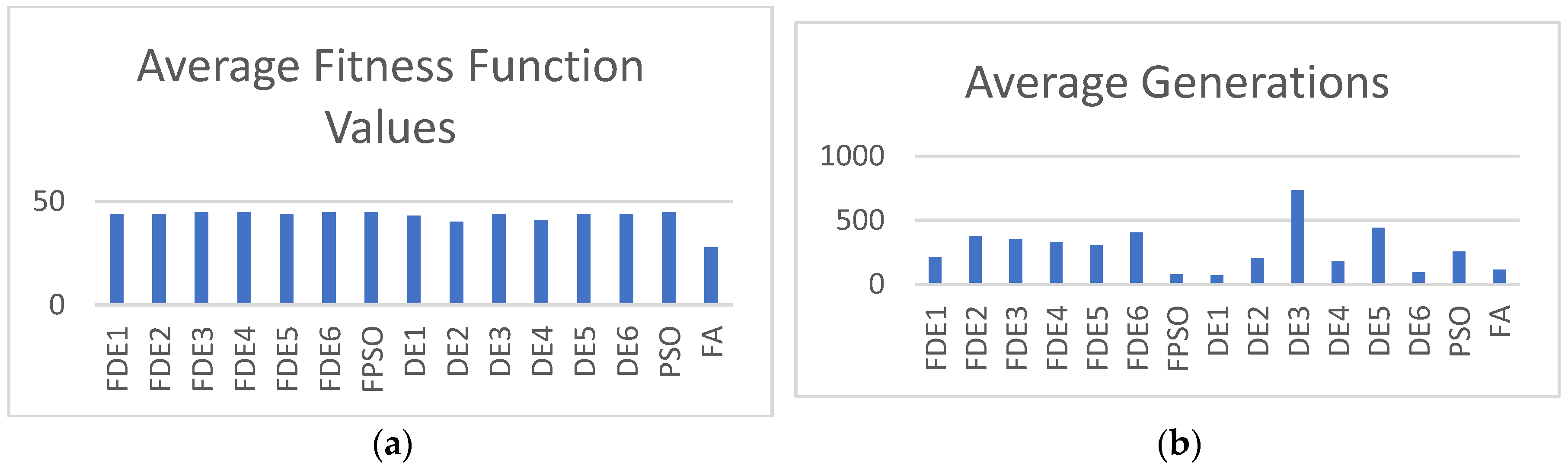
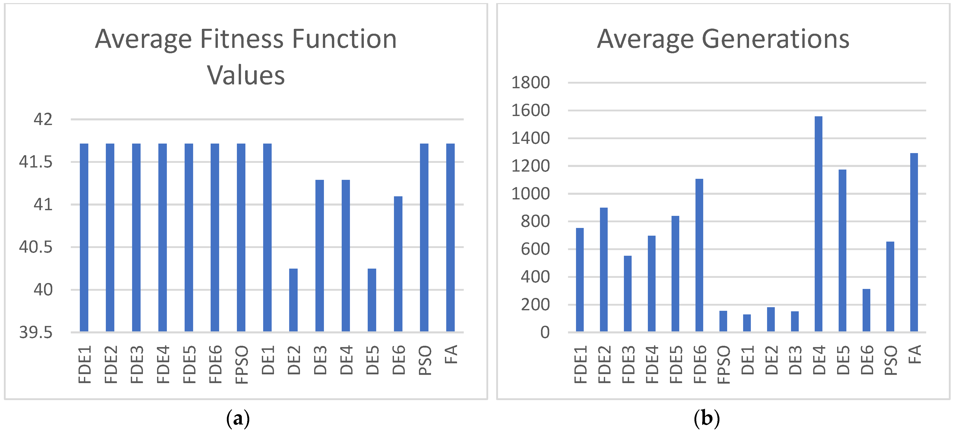
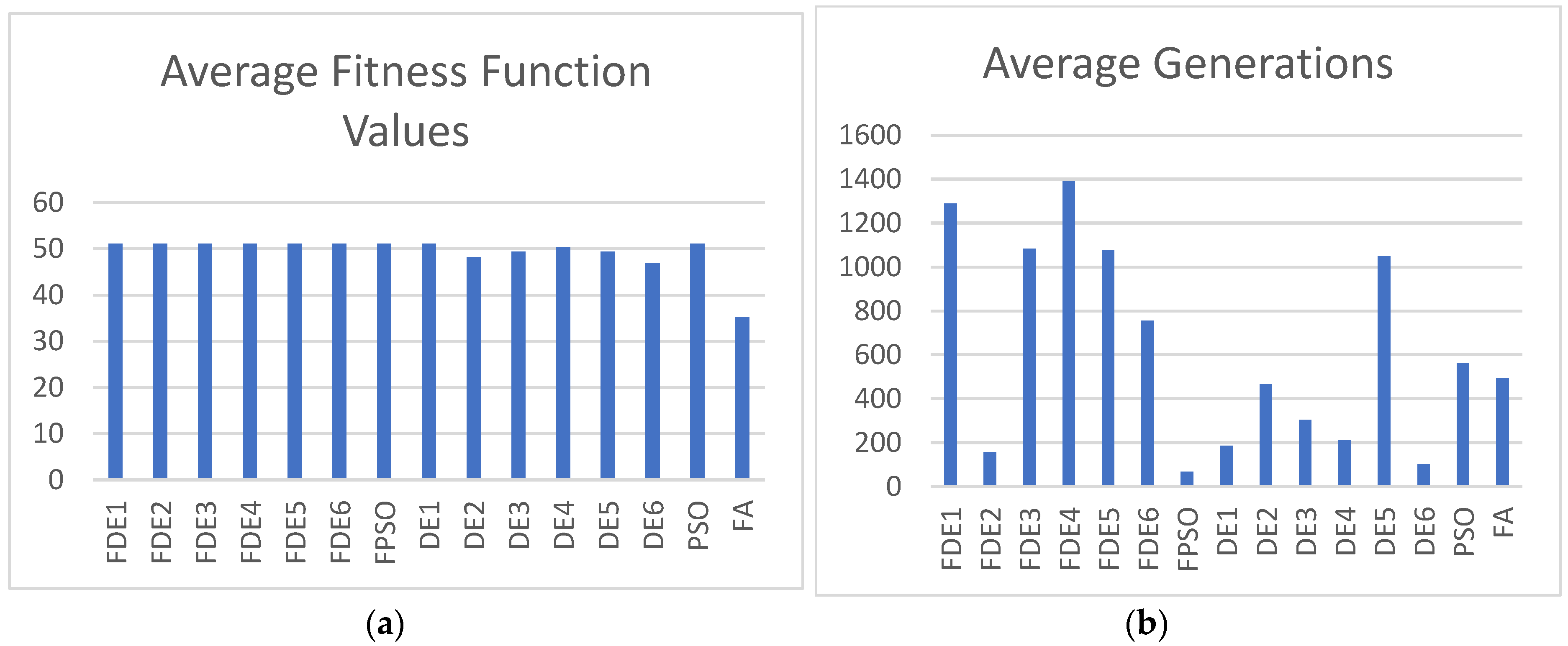
4.1. Comparison of Hybrid Algorithms
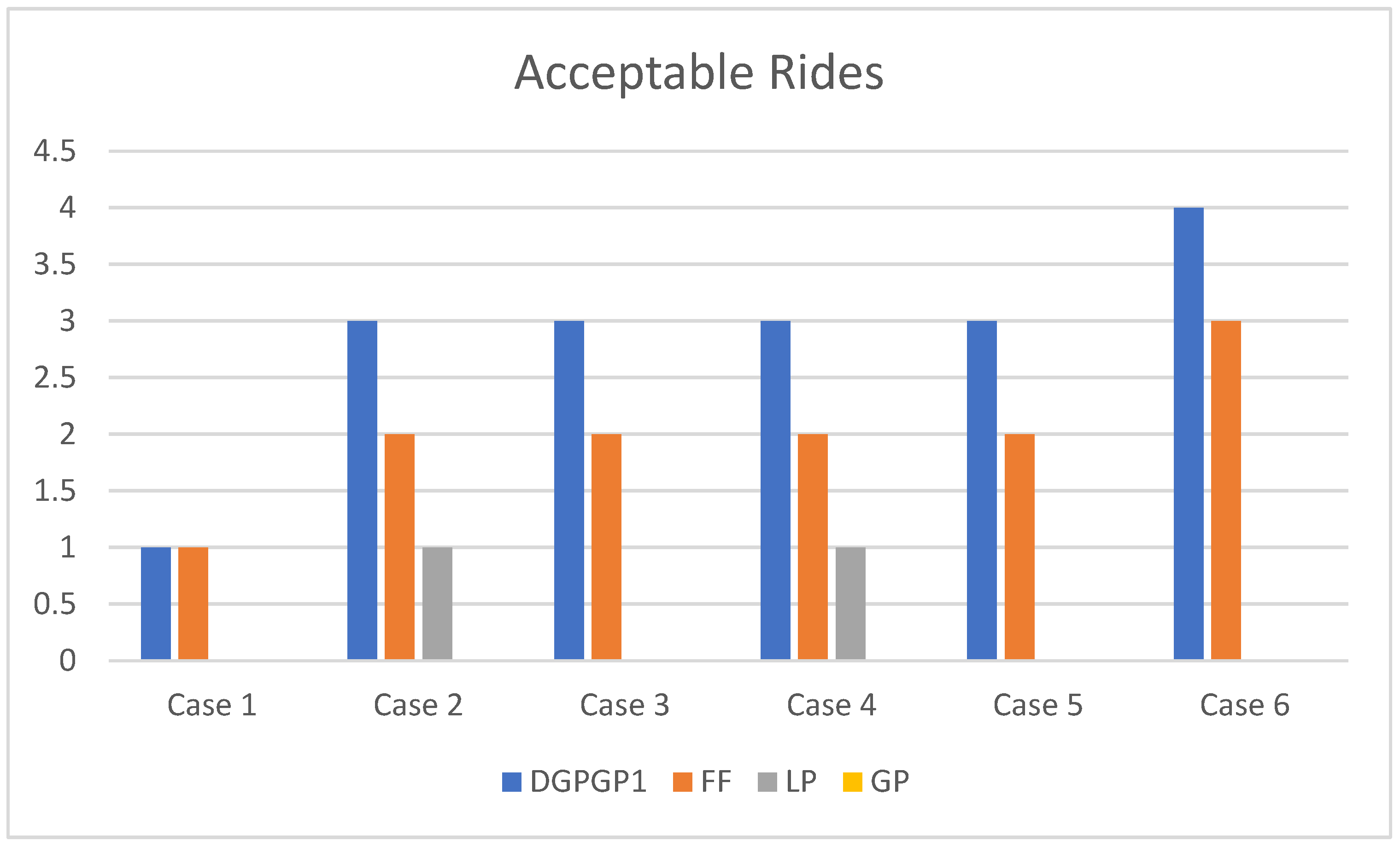
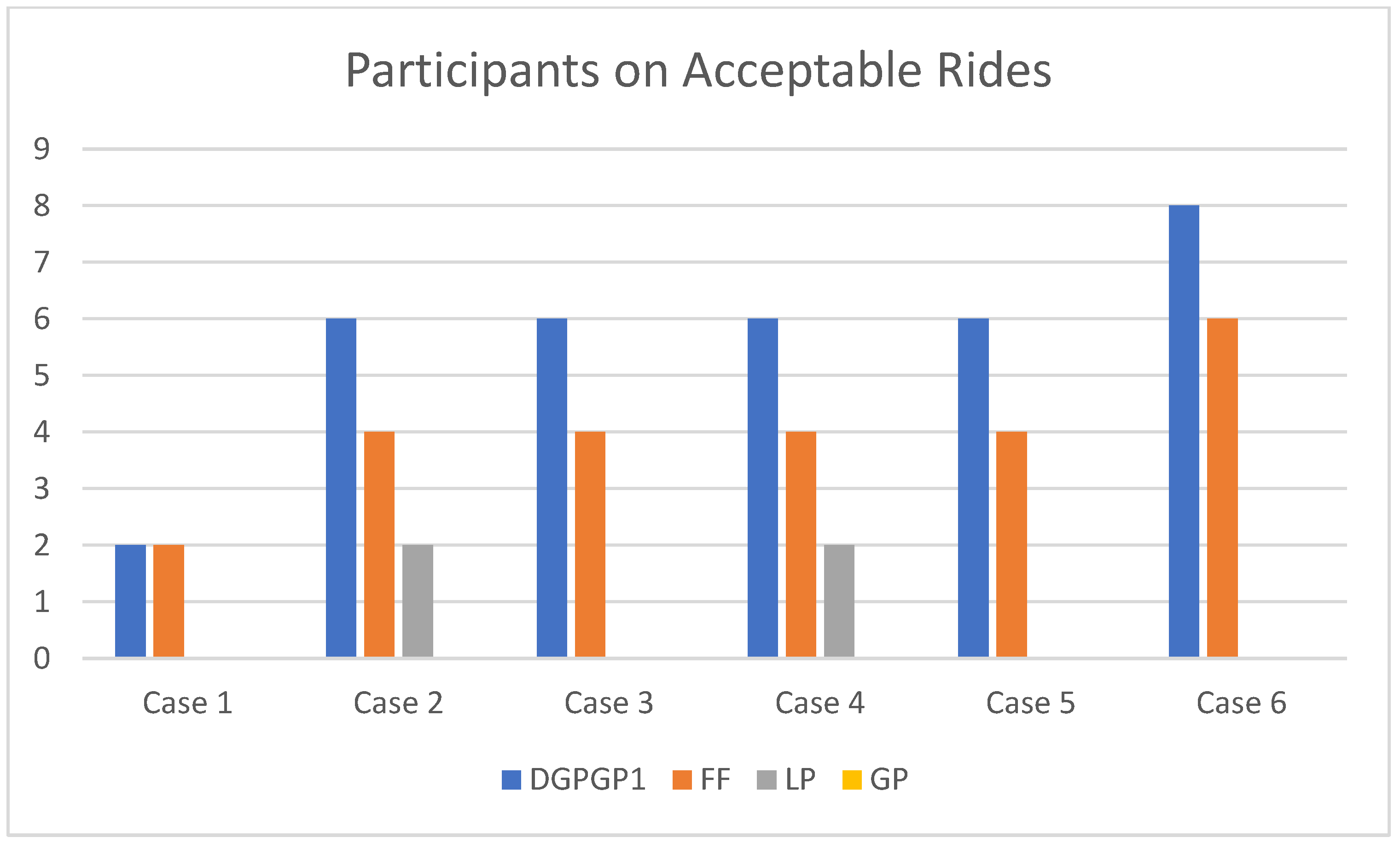
4.2. Comparison of the Proposed Allocation Method with Existing Methods
5. Discussion
6. Conclusions
Funding
Data Availability Statement
Conflicts of Interest
References
- Sustainable Transportation and Fuels. Available online: https://www.energy.gov/eere/sustainable-transportation-and-fuels (accessed on 20 November 2023).
- AGENDA 21. Available online: https://sustainabledevelopment.un.org/content/documents/Agenda21.pdf (accessed on 20 November 2023).
- Plan of Implementation of the World Summit on Sustainable Development. Available online: https://library.arcticportal.org/1679/1/Johannesburg_Plan_of_Implementation.pdf (accessed on 20 November 2023).
- Sustainable Transport. Available online: https://sdgs.un.org/topics/sustainable-transport (accessed on 20 November 2023).
- Transforming Our World: The 2030 Agenda for Sustainable Development. Available online: https://sdgs.un.org/2030agenda (accessed on 20 November 2023).
- Tafreshian, A.; Masoud, N.; Yin, Y. Frontiers in service science: Ride matching for peer-to-peer ride sharing: A review and future directions. Serv. Sci. 2020, 12, 44–60. [Google Scholar] [CrossRef]
- Ferrero, F.; Perboli, G.; Rosano, M.; Vesco, A. Car-sharing services: An annotated review. Sustain. Cities Soc. 2018, 37, 501–518. [Google Scholar] [CrossRef]
- Narayanan, S.; Chaniotakis, E.; Antoniou, C. ‘Shared autonomous vehicle services: A comprehensive review. Transp. Res. C Emerg. Technol. 2020, 111, 255–293. [Google Scholar] [CrossRef]
- Ricci, M. Bike sharing: A review of evidence on impacts and processes of implementation and operation. Res. Transp. Bus. Manag. 2015, 15, 28–38. [Google Scholar] [CrossRef]
- Hao, M.; Yamamoto, T. Shared autonomous vehicles: A review considering car sharing and autonomous vehicles. Asian Transp. Stud. 2018, 5, 47–63. [Google Scholar]
- Mohan, A.; Bruchon, M.; Michalek, J.; Vaishnav, P. Life Cycle Air Pollution, Greenhouse Gas, and Traffic Externality Benefits and Costs of Electrifying Uber and Lyft. Environ. Sci. Technol. 2023, 57, 8524–8535. [Google Scholar] [CrossRef] [PubMed]
- Amatuni, L.; Ottelin, J.; Steubing, B.; Mogollón, J.M. Does car sharing reduce greenhouse gas emissions? Assessing the modal shift and lifetime shift rebound effects from a life cycle perspective. J. Clean. Prod. 2020, 266, 121869. [Google Scholar] [CrossRef]
- Exploring the Impact of Shared Mobility Services on CO2, Environment Working Paper No. 175. Available online: https://one.oecd.org/document/ENV/WKP(2021)7/en/pdf (accessed on 20 November 2023).
- Bruglieri, M.; Ciccarelli, D.; Colorni, A.; Luè, A. PoliUniPool: A carpooling system for universities. Procedia-Soc. Behav. Sci. 2011, 20, 558–567. [Google Scholar] [CrossRef]
- Liftango. Available online: https://www.newcastle.edu.au/our-uni/campuses-and-locations/transport/rideshare-liftango (accessed on 20 November 2023).
- Lyft. Available online: https://www.lyft.com/ (accessed on 20 November 2023).
- Uber. Available online: https://www.uber.com/ (accessed on 20 November 2023).
- Didi. Available online: https://www.didiglobal.com (accessed on 20 November 2023).
- Wingz. Available online: https://www.wingz.me/ (accessed on 20 November 2023).
- Via. Available online: https://ridewithvia.com/ (accessed on 20 November 2023).
- Hwang, K.; Giuliano, G. The Determinants of Ridesharing: Literature Review; Working Paper UCTC No. 38; The University of California Transportation Center: Los Angeles, CA, USA, 1990; Available online: https://escholarship.org/uc/item/3r91r3r4 (accessed on 20 November 2023).
- Wieding, S.V.; Sprei, F.; Hult, C.; Hult, Å.; Roth, A.; Persson, M. Drivers and barriers to business-to-business carsharing for work trips—A case study of Gothenburg, Sweden. Case Stud. Transp. Policy 2022, 10, 2330–2336. [Google Scholar] [CrossRef]
- Agatz, N.; Erera, A.; Savelsbergh, M.; Wang, X. Optimization for dynamic ride-sharing: A review. Eur. J. Oper. Res. 2012, 223, 295–303. [Google Scholar] [CrossRef]
- Mourad, A.; Puchinger, J.; Chu, C. A survey of models and algorithms for optimizing shared mobility. Transp. Res. Part B Methodol. 2019, 123, 323–346. [Google Scholar] [CrossRef]
- Martins, L.D.C.; de la Torre, R.; Corlu, C.G.; Juan, A.A.; Masmoudi, M.A. Optimizing ride-sharing operations in smart sustainable cities: Challenges and the need for agile algorithms. Comput. Ind. Eng. 2021, 153, 107080. [Google Scholar] [CrossRef]
- Saisubramanian, S.; Basich, C.; Zilberstein, S.; Goldman, C.V. Satisfying Social Preferences in Ridesharing Services. In Proceedings of the 2019 IEEE Intelligent Transportation Systems Conference (ITSC), Auckland, New Zealand, 27–30 October 2019; pp. 3720–3725. [Google Scholar]
- Hsieh, F.S. Trust-Based Recommendation for Shared Mobility Systems Based on a Discrete Self-Adaptive Neighborhood Search Differential Evolution Algorithm. Electronics 2022, 11, 776. [Google Scholar] [CrossRef]
- Yang, X.S. Firefly algorithms for multimodal optimization. Lect. Notes Comput. Sci. 2009, 5792, 169–178. [Google Scholar]
- Kennedy, J.; Eberhart, R.C. Particle swarm optimization. In Proceedings of the IEEE International Conference on Neural Networks, Perth, WA, Australia, 27 November–1 December 1995; pp. 1942–1948. [Google Scholar]
- Price, K.; Storn, R.; Lampinen, J. Differential Evolution: A Practical Approach to Global Optimization; Springer: Berlin/Heidelberg, Germany, 2005. [Google Scholar]
- Hsieh, F.-S. A Self-Adaptive Meta-Heuristic Algorithm Based on Success Rate and Differential Evolution for Improving the Performance of Ridesharing Systems with a Discount Guarantee. Algorithms 2024, 17, 9. [Google Scholar] [CrossRef]
- Li, J. A Hybrid Differential Evolution Method for Practical Engineering Problems. In Proceedings of the 2009 IITA International Conference on Control, Automation and Systems Engineering (Case 2009), Zhangjiajie, China, 11–12 July 2009; pp. 54–57. [Google Scholar] [CrossRef]
- Zhang, L.; Liu, L.; Yang, X.S.; Dai, Y. A Novel Hybrid Firefly Algorithm for Global Optimization. PLoS ONE 2016, 11, e0163230. [Google Scholar] [CrossRef] [PubMed]
- Paital, S.R.; Ray, P.K.; Mohanty, A. Firefly-swarm optimized fuzzy adaptive PSS in power system for transient stability enhancement. In Proceedings of the 2017 Progress in Electromagnetics Research Symposium-Fall (PIERS-FALL), Singapore, 19–22 November 2017; pp. 1969–1976. [Google Scholar]
- Paital, S.R.; Mohanty, A.; Eddy Foo, Y.S.; Krishnan, A.; Beng Gooi, H.; Amaratunga, G.A.J. A Hybrid Firefly-Swarm Optimized Fractional Order Interval Type-2 Fuzzy PID-PSS for Transient Stability Improvement. IEEE Trans. Ind. Appl. 2019, 55, 6486–6498. [Google Scholar]
- Ibrahim, I.M.; Omran, W.A.; Abdelaziz, A.Y. Optimal Sizing of Microgrid System Using Hybrid Firefly and Particle Swarm Optimization Algorithm. In Proceedings of the 22nd International Middle East Power Systems Conference (MEPCON), Assiut, Egypt, 14–16 December 2021; pp. 287–293. [Google Scholar] [CrossRef]
- Aydilek, İ.B. A hybrid firefly and particle swarm optimization algorithm for computationally expensive numerical problems. Appl. Soft Comput. 2018, 66, 232–249. [Google Scholar] [CrossRef]
- Hsieh, F.-S. A Hybrid Firefly-DE algorithm for Ridesharing Systems with Cost Savings Allocation Schemes. In Proceedings of the 2022 IEEE World AI IoT Congress (AIIoT), Seattle, WA, USA, 6–9 June 2022; pp. 649–653. [Google Scholar]
- Hsieh, F.-S. Improve Decision Making Efficiency in Ridesharing Systems through a Hybrid Firefly-PSO algorithm. In Proceedings of the 2023 IEEE World AI IoT Congress (AIIoT), Seattle, WA, USA, 7–10 June 2023; pp. 578–582. [Google Scholar]
- Guajardoa, M.; Ronnqvist, M. A review on cost allocation methods in collaborative transportation. Int. Trans. Oper. Res. 2016, 23, 371–392. [Google Scholar] [CrossRef]
- Shapley, L.S. A Value for N-Person Games. Available online: https://www.rand.org/content/dam/rand/pubs/papers/2021/P295.pdf (accessed on 20 November 2023).
- Schmeidler, D. The Nucleolus of a Characteristic Function Game. SIAM J. Appl. Math. 1969, 17, 1163–1170. [Google Scholar] [CrossRef]
- Kalai, E. Proportional solutions to bargaining situations: Intertemporal utility comparisons. Econometrica 1977, 45, 1623–1630. [Google Scholar] [CrossRef]
- Wang, X.; Agatz, N.; Erera, A. Stable Matching for Dynamic Ride-Sharing Systems. Transp. Sci. 2018, 52, 850–867. [Google Scholar] [CrossRef]
- Agatz, N.A.H.; Erera, A.L.; Savelsbergh, M.W.P.; Wang, X. Dynamic ride-sharing: A simulation study in metro Atlanta. Transp. Res. Part B Methodol. 2011, 45, 1450–1464. [Google Scholar] [CrossRef]
- Hsieh, F.S.; Zhan, F.; Guo, Y. A solution methodology for carpooling systems based on double auctions and cooperative coevolutionary particle swarms. Appl. Intell. 2019, 49, 741–763. [Google Scholar] [CrossRef]
- Hsieh, F.-S. A Comparison of Three Ridesharing Cost Savings Allocation Schemes Based on the Number of Acceptable Shared Rides. Energies 2021, 14, 6931. [Google Scholar] [CrossRef]
- Hsieh, F.-S. Improving Acceptability of Cost Savings Allocation in Ridesharing Systems Based on Analysis of Proportional Methods. Systems 2023, 11, 187. [Google Scholar] [CrossRef]
- Ravindran, A.; Ragsdell, K.M.; Reklaitis, G.V. Enginering Optimization: Methods and Applications, 2nd ed.; Wiley: New York, NY, USA, 2007. [Google Scholar]
- Deb, K. An efficient constraint handling method for genetic algorithms. Comput. Methods Appl. Mech. Eng. 2000, 186, 311–338. [Google Scholar] [CrossRef]


| Variable | Meaning |
|---|---|
| the number of passengers. | |
| passenger index, . | |
| the number of drivers. | |
| driver index, . | |
| location index, . | |
| the number of bids submitted by driver, . | |
| bid index of a driver, , . | |
| the -th bid of driver with = , where : number of seats allocated to passenger ’s pick-up location; : number of seats released at passenger ’s drop-off location; : driver original cost of -th bid of driver without ridesharing; : the transport cost of -th bid of driver . : the set of passengers on the ride of the -th bid of driver | |
| the bid of passenger with = , where : number of seats requested for passenger k’s pick-up location; : number of seats released for passenger k’s drop-off location; : original cost of passenger p without ridesharing. | |
| decision variable for the bid of driver ; = 1 if the bid of driver is a winning bid; otherwise, = 0 if the bid of driver is not a winning bid. | |
| decision variable for passenger ; = 1 if the bid of passenger is a winning bid, and = 0 if the bid of passenger is not a winning bid. | |
| share value of ridesharing information provider. | |
| share value of passenger . | |
| share value of driver . | |
| the objective function for cost savings: |
| Method | Stakeholder | Share Value | |
|---|---|---|---|
| Driver Group–Passenger Group Proportional (DGPGP) Method | information provider | (8) | |
| passenger | , where | (9) | |
| driver | , where | (10) |
| Variable | Meaning |
|---|---|
| the fitness function, | |
| the set of feasible solutions in the current population | |
| the objective function value of the worst feasible solution in , | |
| the function to evaluate infeasible solution | |
| population size | |
| the index of an individual in the population, | |
| the dimension of the problem | |
| the -th individual in the population, where | |
| the value of the -th dimension of the -th individual, where | |
| and | |
| the best individual in the current population | |
| the value of the -th dimension of the candidate vector generated for the -th individual, where and | |
| the total number of generations | |
| the index of generation | |
| the distance between firefly and firefly | |
| the light absorption coefficient | |
| the attractiveness when the distance between firefly and firefly is zero | |
| the attractiveness for the distance between firefly and firefly | |
| a random number drawn from a uniform distribution in [0, 1] | |
| a constant parameter in [0, 1] | |
| = , a function to transform a real value into a value in [0, 1] | |
| a random variable with uniform distribution, | |
| a random variable with uniform distribution, | |
| cognitive acceleration coefficient, which is a non-negative real parameter less than 1 | |
| social acceleration coefficient, which is a non-negative real parameter less than 1 | |
| the personal best of particle at time , where , and is the -th element of the vector , where . | |
| the global best, and is the -th element of the vector , where | |
| the procedure to map a real value to zero or one defined in Procedure 1 | |
| Gaussian distribution with mean 0 and standard deviation 1.0 | |
| the scale factor, which is generated from Gaussian distribution | |
| the crossover rate |
| Approach | The Way to Create the n-th Element of Trial Vector | |
|---|---|---|
| PSO | Step 1: Generate random numbers and with uniform distribution Step 2: Calculate the -th dimension of trial vector | (12) |
| DE1 | Step 1: Generate numbers , and from {1,2,…, } randomly Step 2: Calculate the -th element, , of mutant vector Step 3: Calculate the -th dimension of trial vector by applying the crossover operation | (13) |
| DE2 | Step 1: Generate numbers and from {1,2,…, } randomly Step 2: Calculate the -th element, , of mutant vector Step 3: Calculate the -th dimension of trial vector by applying the crossover operation | (14) |
| DE3 | Step 1: Generate numbers , , , and from {1,2,…, } randomly Step 2: Calculate the -th element, , of mutant vector Step 3: Calculate the -th dimension of trial vector by applying the crossover operation | (15) |
| DE4 | Step 1: Generate numbers , , and from {1,2,…, } randomly Step 2: Calculate the -th element, , of mutant vector Step 3: Calculate the -th dimension of trial vector by applying the crossover operation | (16) |
| DE5 | Step 1: Generate numbers and from {1,2,…, } randomly Step 2: Calculate the -th element, , of mutant vector Step 3: Calculate the -th dimension of trial vector by applying the crossover operation | (17) |
| DE6 | Step 1: Generate numbers , , and from {1,2,…, } randomly Step 2: Calculate the -th element, , of mutant vector Step 3: Calculate the -th dimension of trial vector by applying the crossover operation | (18) |
| DE1 | DE2 | DE3 | DE4 | DE5 | DE6 | PSO | FA |
|---|---|---|---|---|---|---|---|
| = 0.5 | = 0.5 | = 0.5 | = 0.5 | = 0.5 | = 0.5 | = 0.4 | = 1.0 |
| : generated from Gaussian distribution | : generated from Gaussian distribution | : generated from Gaussian distribution | : generated from Gaussian distribution | : generated from Gaussian distribution | : generated from Gaussian distribution | = 0.4 = 0.6 | = 0.2 = 0.2 |
| = 50,000 | = 50,000 | = 50,000 | = 50,000 | = 50,000 | = 50,000 | = 50,000 | = 50,000 |
| = 4 | = 4 | = 4 | = 4 | = 4 | = 4 | = 4 | = 4 |
| = 10/30 | = 10/30 | = 10/30 | = 10/30 | = 10/30 | = 10/30 | = 10/30 | = 10/30 |
| FDE1 | FDE2 | FDE3 | FDE4 | FDE5 | FDE6 | FPSO |
|---|---|---|---|---|---|---|
| Parameters are the same as DE1 and FA | Parameters are the same as DE2 and FA | Parameters are the same as DE3 and FA | Parameters are the same as DE4 and FA | Parameters are the same as DE5 and FA | Parameters are the same as DE6 and FA | Parameters are the same as PSO and FA |
| Case | D | P | FDE1 | FDE2 | FDE3 | FDE4 | FDE5 | FDE6 | FPSO |
|---|---|---|---|---|---|---|---|---|---|
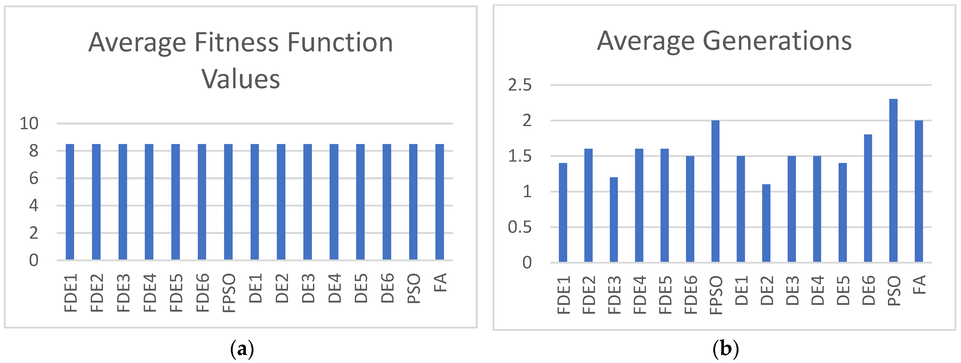
| 1 | 1 | 4 | 8.495/1.8 | 8.495/2.3 | 8.495/2.2 | 8.495/2.6 | 8.495/2.6 | 8.495/3.1 | 8.495/1.9 |
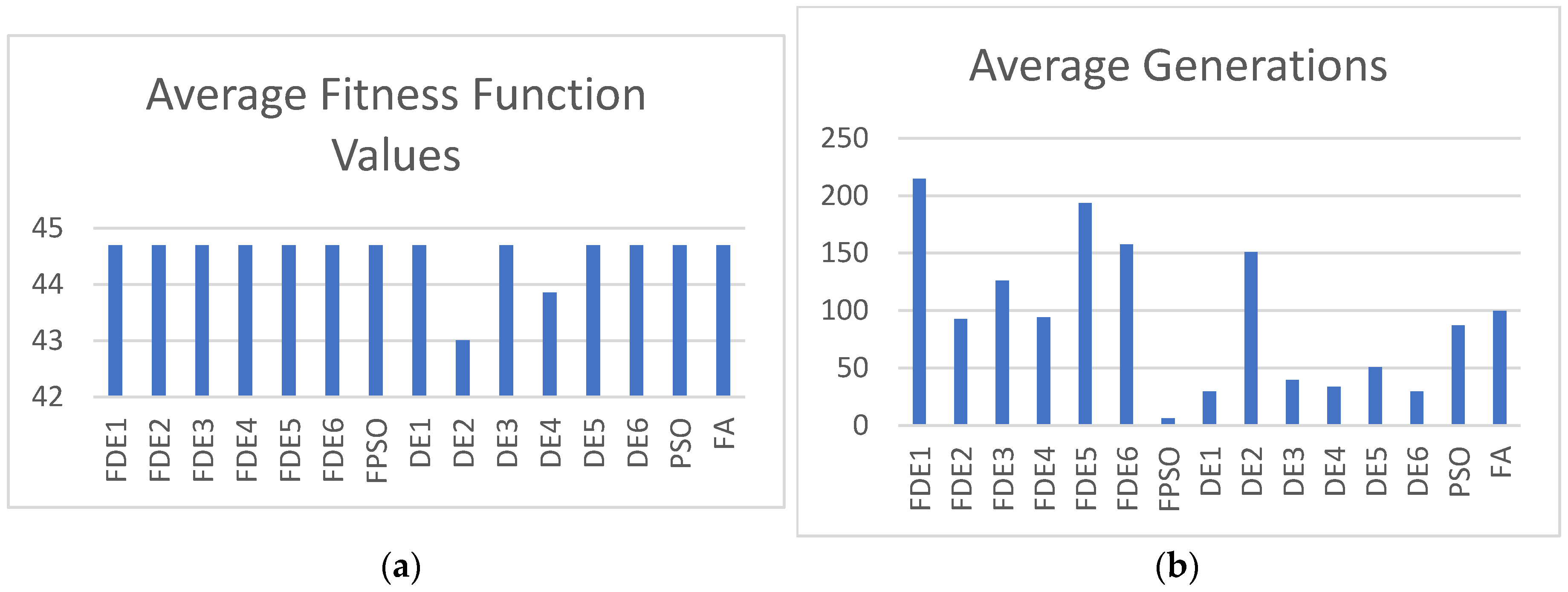
| 2 | 3 | 10 | 43.8523/211.7 | 43.8523/377.5 | 44.7/348.8 | 44.7/329 | 43.8523/305.3 | 44.7/404.4 | 44.7/77.6 |
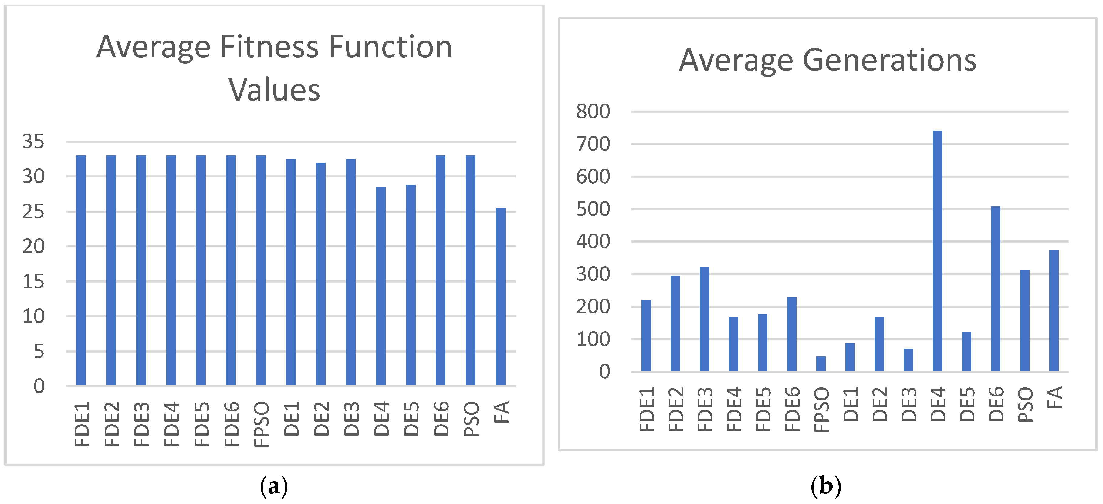
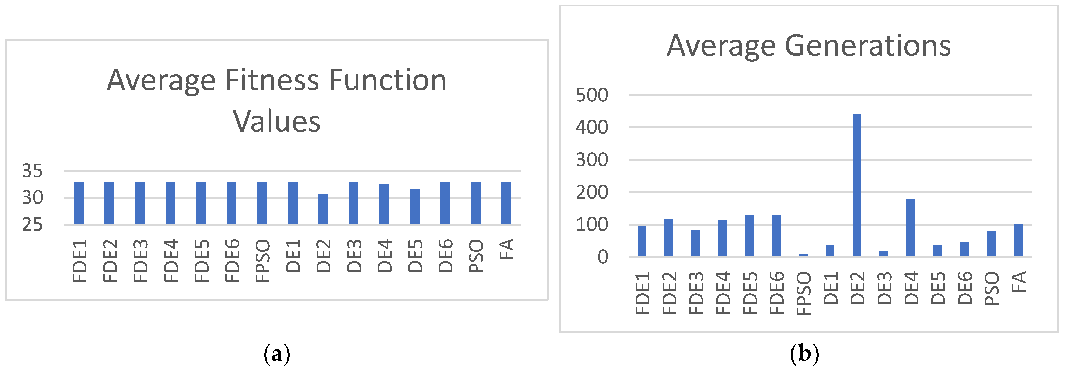
| 3 | 3 | 10 | 32.998/220.4 | 32.998/294.7 | 32.998/322.9 | 32.998/168.8 | 32.998/176.4 | 32.998/229.3 | 32.998/46.2 |
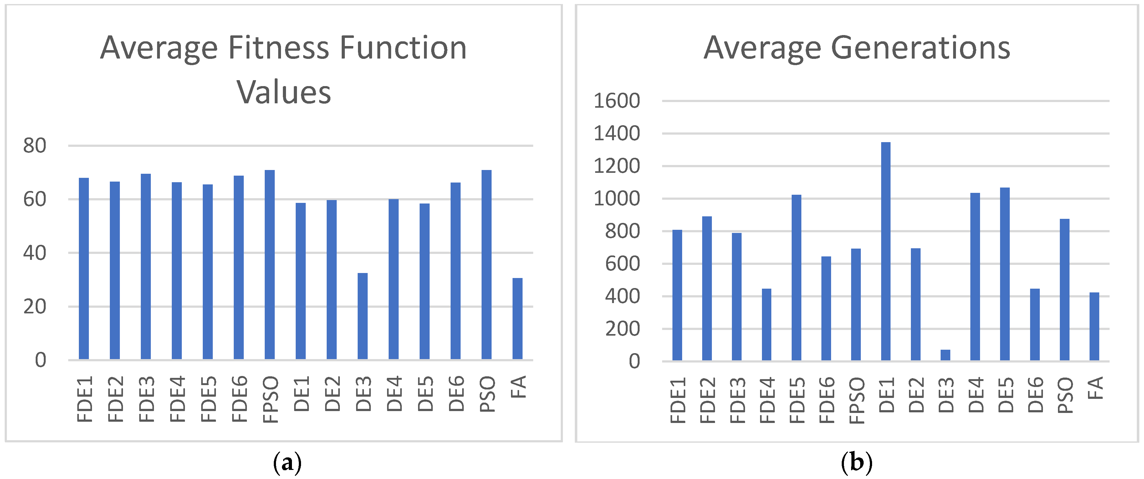
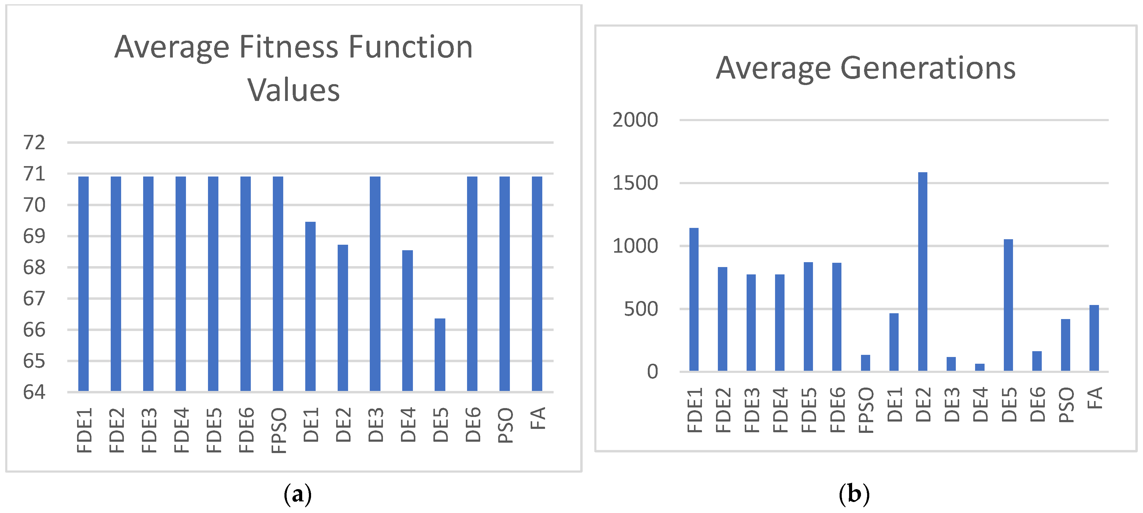
| 4 | 5 | 11 | 67.992/807 | 66.533/891.2 | 69.451/789 | 66.3698/445.8 | 65.4771/1022.6 | 68.7215/644.3 | 70.91/692.9 |
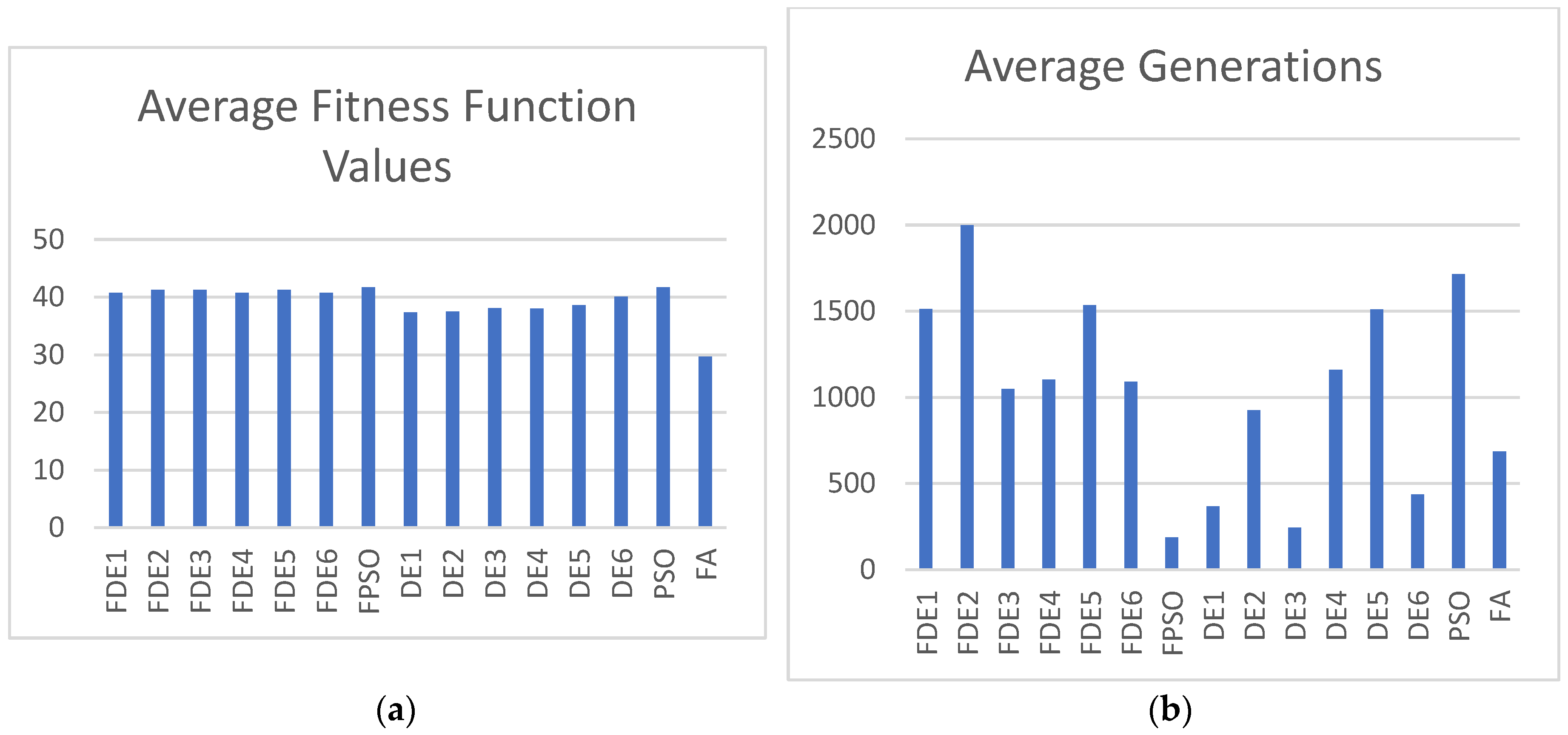
| 5 | 5 | 12 | 40.7687/1512 | 41.2418/1999.4444 | 41.2418/1049.8888 | 40.7687/1103.5555 | 41.2418/1535.2222 | 40.7687/1090.7777 | 41.715/187.3333 |
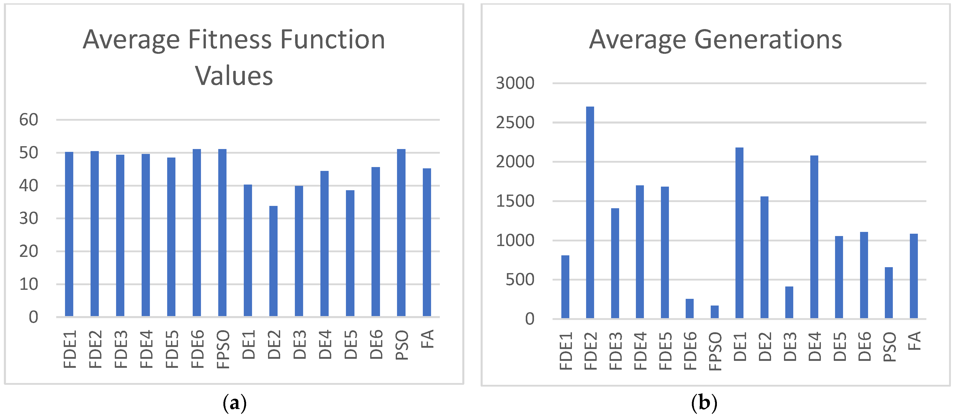
| 6 | 6 | 12 | 50.2144/807.4444 | 50.4383/2702 | 49.3616/1407.5555 | 49.5855/1697.888 | 48.5088/1681.7777 | 51.11/256.1111 | 51.11/171.5555 |
| Case | D | P | DE1 | DE2 | DE3 | DE4 | DE5 | DE6 | PSO | FA |
|---|---|---|---|---|---|---|---|---|---|---|
| 1 | 1 | 4 | 8.495/3.4 | 8.495/2.5 | 8.495/3.1 | 8.495/2.7 | 8.495/8.6 | 8.495/1.9 | 8.495/4.4 | 8.495/2.7 |
| 2 | 3 | 10 | 43.006/71.5 | 40.1207/205.1 | 43.8523/733.6 | 40.9684/181.5 | 43.8523/439.7 | 43.8523/94.9 | 44.7/255 | 27.8061/115.3 |
| 3 | 3 | 10 | 32.4747/87.4 | 31.9514/166.7 | 32.4747/70.7 | 28.553/741.8 | 28.8135/122.2 | 32.998/508.5 | 32.998/313 | 25.4751/375.4 |
| 4 | 5 | 11 | 58.6415/1345.9 | 59.6974/693.8 | 32.4747/70.7 | 59.9814/1034.5 | 58.3949/1068.4 | 66.1931/446.6 | 70.91/875 | 30.5676/423 |
| 5 | 5 | 12 | 37.3519/368.4 | 37.5104/924.6 | 38.1275/243.9 | 38.0337/1160.4 | 38.5859/1510.6 | 40.0552/435.1 | 41.715/1716.1111 | 29.6832/684.6666 |
| 6 | 6 | 12 | 40.2843/2179.9 | 33.7963/1558.2 | 39.865/413.9 | 44.4525/2078.6 | 38.5798/1052.7 | 45.6008/1107.9 | 51.11/657 | 45.2088/1084.4444 |
| Case | D | P | FDE1 | FDE2 | FDE3 | FDE4 | FDE5 | FDE6 | FPSO |
|---|---|---|---|---|---|---|---|---|---|
| 1 | 1 | 4 | 8.495/1.4 | 8.495/1.6 | 8.495/1.2 | 8.495/1.6 | 8.495/1.6 | 8.495/1.5 | 8.495/2 |
| 2 | 3 | 10 | 44.7/214.6 | 44.7/92.7 | 44.7/125.9 | 44.7/93.9 | 44.7/193.6 | 44.7/157.6 | 44.7/6.3 |
| 3 | 3 | 10 | 32.998/93.6 | 32.998/117 | 32.998/83.3 | 32.998/115.7 | 32.998/131 | 32.998/130.6 | 32.998/9.8 |
| 4 | 5 | 11 | 70.91/1141.7 | 70.91/829.9 | 70.91/773.6 | 70.91/773.8 | 70.91/870 | 70.91/864.7 | 70.91/133.6 |
| 5 | 5 | 12 | 41.715/753.4 | 41.715/899.3 | 41.715/552.1 | 41.715/697.7 | 41.715/840.6 | 41.715/1106.2 | 41.715/154.9 |
| 6 | 6 | 12 | 51.11/1288.6 | 51.11/155.3 | 51.11/1083.2 | 51.11/1392.7 | 51.11/1076.1 | 51.11/755.5 | 51.11/68.1 |
| Case | D | P | DE1 | DE2 | DE3 | DE4 | DE5 | DE6 | PSO | FA |
|---|---|---|---|---|---|---|---|---|---|---|
| 1 | 1 | 4 | 8.495/1.5 | 8.495/1.1 | 8.495/1.5 | 8.495/1.5 | 8.495/1.4 | 8.495/1.8 | 8.495/2.3 | 8.495/2 |
| 2 | 3 | 10 | 44.7/29.4 | 43.0046/150.7 | 44.7/39.6 | 43.8523/33.5 | 44.7/50.7 | 44.7/29.6 | 44.7/87 | 44.7/99.5 |
| 3 | 3 | 10 | 32.998/37.7 | 30.6441/440.9 | 32.998/17 | 32.4747/177.9 | 31.5101/37.4 | 32.998/46.6 | 32.998/80.2 | 32.998/100.5 |
| 4 | 5 | 11 | 69.451/464.2 | 68.7215/1584.3 | 70.91/117.9 | 68.5448/63.3 | 66.3563/1052.9 | 70.91/163.2 | 70.91/418.6 | 70.91/529.9 |
| 5 | 5 | 12 | 41.715/128.5 | 40.2464/181.2 | 41.2892/151.5 | 41.2892/1557 | 40.2464/1172.8 | 41.098/312.2 | 41.715/654.8 | 41.715/1291.4 |
| 6 | 6 | 12 | 51.11/185.7 | 48.1973/465 | 49.3735/303.9 | 50.3425/211.3 | 49.3735/1049.2 | 46.9785/101 | 51.11/560.2 | 35.177/492.5 |
| Case | D | P | DGPGP1 | DGPGP2 | FF | LP | GP | ||
|---|---|---|---|---|---|---|---|---|---|
| 1 | 1 | 4 | 1/2 | 0/0 | 1/2 | 0/0 | 0/0 | 0.05 | 0.3 |
| 2 | 3 | 10 | 3/6 | 0/0 | 2/4 | 1/2 | 0/0 | 0.12 | 0.5 |
| 3 | 3 | 10 | 3/6 | 0/0 | 2/4 | 0/0 | 0/0 | 0.1 | 0.2 |
| 4 | 5 | 11 | 3/6 | 0/0 | 2/4 | 1/2 | 0/0 | 0.1 | 0.3 |
| 5 | 5 | 12 | 3/5 | 0/0 | 2/4 | 0/0 | 0/0 | 0.12 | 0.3 |
| 6 | 6 | 12 | 4/8 | 0/0 | 3/6 | 0/0 | 0/0 | 0.11 | 0.3 |
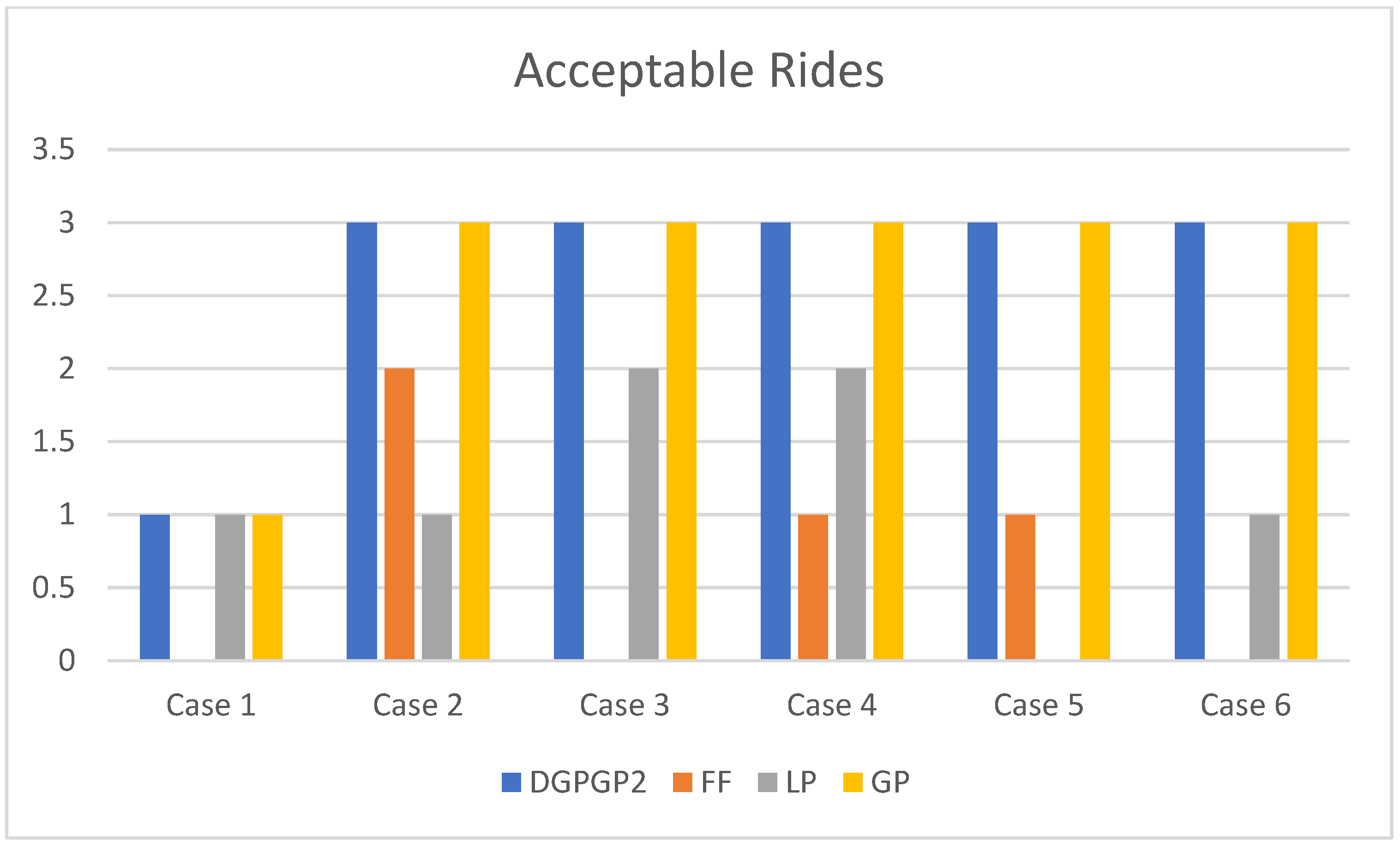
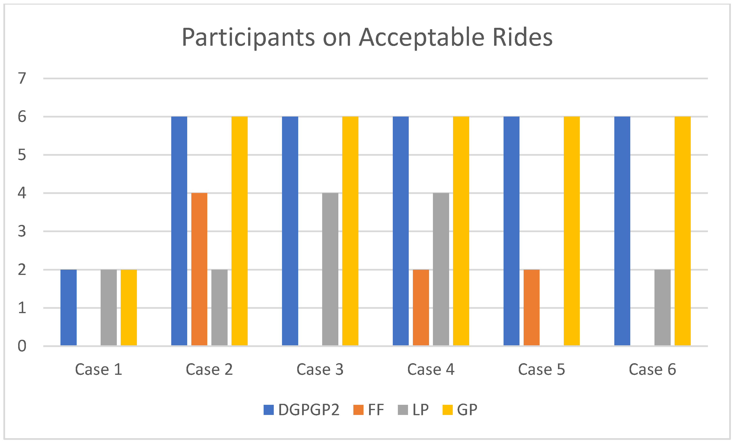
| Case | D | P | DGPGP1 | DGPGP2 | FF | LP | GP | ||
|---|---|---|---|---|---|---|---|---|---|
| 1 | 1 | 4 | 0/0 | 1/2 | 0/0 | 1/2 | 1/2 | 0.1 | 0.1 |
| 2 | 3 | 10 | 0/0 | 3/6 | 2/4 | 1/2 | 3/6 | 0.2 | 0.2 |
| 3 | 3 | 10 | 0/0 | 3/6 | 0/0 | 2/4 | 3/6 | 0.15 | 0.15 |
| 4 | 5 | 11 | 0/0 | 3/6 | 1/2 | 2/4 | 3/6 | 0.2 | 0.2 |
| 5 | 5 | 12 | 0/0 | 3/6 | 1/2 | 0/0 | 3/6 | 0.15 | 0.15 |
| 6 | 6 | 12 | 0/0 | 3/6 | 0/0 | 1/2 | 3/6 | 0.2 | 0.2 |
Disclaimer/Publisher’s Note: The statements, opinions and data contained in all publications are solely those of the individual author(s) and contributor(s) and not of MDPI and/or the editor(s). MDPI and/or the editor(s) disclaim responsibility for any injury to people or property resulting from any ideas, methods, instructions or products referred to in the content. |
© 2024 by the author. Licensee MDPI, Basel, Switzerland. This article is an open access article distributed under the terms and conditions of the Creative Commons Attribution (CC BY) license (https://creativecommons.org/licenses/by/4.0/).
Share and Cite
Hsieh, F.-S. Comparison of a Hybrid Firefly–Particle Swarm Optimization Algorithm with Six Hybrid Firefly–Differential Evolution Algorithms and an Effective Cost-Saving Allocation Method for Ridesharing Recommendation Systems. Electronics 2024, 13, 324. https://doi.org/10.3390/electronics13020324
Hsieh F-S. Comparison of a Hybrid Firefly–Particle Swarm Optimization Algorithm with Six Hybrid Firefly–Differential Evolution Algorithms and an Effective Cost-Saving Allocation Method for Ridesharing Recommendation Systems. Electronics. 2024; 13(2):324. https://doi.org/10.3390/electronics13020324
Chicago/Turabian StyleHsieh, Fu-Shiung. 2024. "Comparison of a Hybrid Firefly–Particle Swarm Optimization Algorithm with Six Hybrid Firefly–Differential Evolution Algorithms and an Effective Cost-Saving Allocation Method for Ridesharing Recommendation Systems" Electronics 13, no. 2: 324. https://doi.org/10.3390/electronics13020324