A Method for Unseen Object Six Degrees of Freedom Pose Estimation Based on Segment Anything Model and Hybrid Distance Optimization

Abstract

Six degrees of freedom pose estimation technology constitutes the cornerstone for precise robotic control and similar tasks. Addressing the limitations of current 6-DoF pose estimation methods in handling object occlusions and unknown objects, we have developed a novel two-stage 6-DoF pose estimation method that integrates RGB-D data with CAD models. Initially, targeting high-quality zero-shot object instance segmentation tasks, we innovated the CAE-SAM model based on the SAM framework. In addressing the SAM model’s boundary blur, mask voids, and over-segmentation issues, this paper introduces innovative strategies such as local spatial-feature-enhancement modules, global context markers, and a bounding box generator. Subsequently, we proposed a registration method optimized through a hybrid distance metric to diminish the dependency of point cloud registration algorithms on sensitive hyperparameters. Experimental results on the HQSeg-44K dataset substantiate the notable improvements in instance segmentation accuracy and robustness rendered by the CAE-SAM model. Moreover, the efficacy of this two-stage method is further corroborated using a 6-DoF pose dataset of workpieces constructed with CloudCompare and RealSense. For unseen targets, the ADD metric achieved 2.973 mm, and the ADD-S metric reached 1.472 mm. This paper significantly enhances pose estimation performance and streamlines the algorithm’s deployment and maintenance procedures.

1. Introduction

In modern robotics, computer vision, and automation, the target six degrees of freedom (6-DoF) pose estimation has been a significant topic of interest [1,2]. Pose estimation determines an object’s location and orientation within a three-dimensional space, typically represented as Euler angles, quaternions, or transformation matrices [3,4]. This issue holds pivotal importance in numerous applications, such as industrial automation, unmanned aerial vehicle navigation, robotic manipulation, and virtual reality. Accurate 6-DOF pose estimation is crucial for achieving precise control and navigation, object tracking, and environmental modeling tasks [5].

Recent years have witnessed notable advancements in machine vision systems in 6-DoF pose estimation. According to the input data type, these methods can be summarized into several typical method types: RGB-based [6,7,8,9,10,11,12,13], depth-based [14,15], RGB-D-based [16,17,18,19,20,21,22], and point cloud-based [23,24,25]. RGB-based methods primarily estimate the pose of an object by analyzing color images, benefiting from high-resolution and rich texture information. They use traditional feature-matching techniques or modern deep learning architectures to extract features, employing Perspective-n-Point (PnP) or least squares algorithms for pose estimation. However, the performance of these methods can be limited when dealing with objects with scarce textures, repetitive patterns, or varying lighting conditions. Depth-based methods, employing depth information acquired by 3D sensors, allow direct estimation of an object’s pose from three-dimensional geometric data. These methods are often combined with Iterative Closest Point (ICP) algorithms [26] or model-based registration techniques, offering strong resistance to interference. RGB-D-based methods merge the advantages of color images and depth information, aiming to utilize the complementarity of these two data modes to enhance the accuracy and robustness of pose estimation. The application of deep learning in this field is increasingly prevalent, especially in networks designed for multimodal fusion capable of learning the most effective way of feature extraction from both types of data. Point cloud-based methods directly process data from 3D scanners or stereoscopic vision systems. Although point cloud data provide direct information about the object’s surface geometry, its unstructured nature and the computational demands for processing are the primary challenges that these methods must overcome. In the paper progress of these methods, using Computer-Aided Design (CAD) models has become a vital technique. Not only can they assist in generating annotated data, but by integrating with actual images or point cloud data, they enhance the accuracy and reliability of pose estimation. Additionally, CAD models support the generation of a substantial amount of synthetic training data, which is particularly crucial for training deep learning models to achieve better generalization performance.

Despite certain advancements in the field of 6-DoF pose estimation achieved by various methods, these technologies still need to overcome several pervasive challenges. These include handling object occlusions in complex scenes and the generalization capabilities of models for unseen objects. Furthermore, many existing 6-DoF pose estimation algorithms rely on precise target masks, which are often provided by publicly available datasets in academic research. However, in real-world scenarios, masks must be obtained through supervised learning methods from manually annotated data, which is both time-consuming and costly. With the continuous emergence of new environments and unknown objects, there is a constant need for data collection and re-annotation. On the other hand, the robustness of 6-DoF pose estimation algorithms dramatically depends on the accuracy of mask prediction, which is a highly challenging task in complex scenarios.

The advent of the Segment Anything Model (SAM) model [27] offers a new approach to the problem of target instance segmentation in new scenes, enabling segmentation of any object in a scene without the need for zero-shot training. Considering the widespread use of consumer-grade RGB-D cameras and the availability of CAD models in industrial settings, this paper explores a 6-DoF pose estimation algorithm based on RGB-D data and CAD models. We employ an enhanced SAM model, allowing for high-quality segmentation of targets without predefined category labels. Furthermore, point clouds generated from depth information are directly geometrically registered with pre-existing CAD models, eliminating the need for any feature learning, complex preprocessing steps, or additional hyperparameter settings. This strategy reduces the algorithm’s dependence on large-scale, high-quality training sets and speeds up the convenience of algorithm deployment and maintenance.

To summarize, the main contributions of this work are as follows:

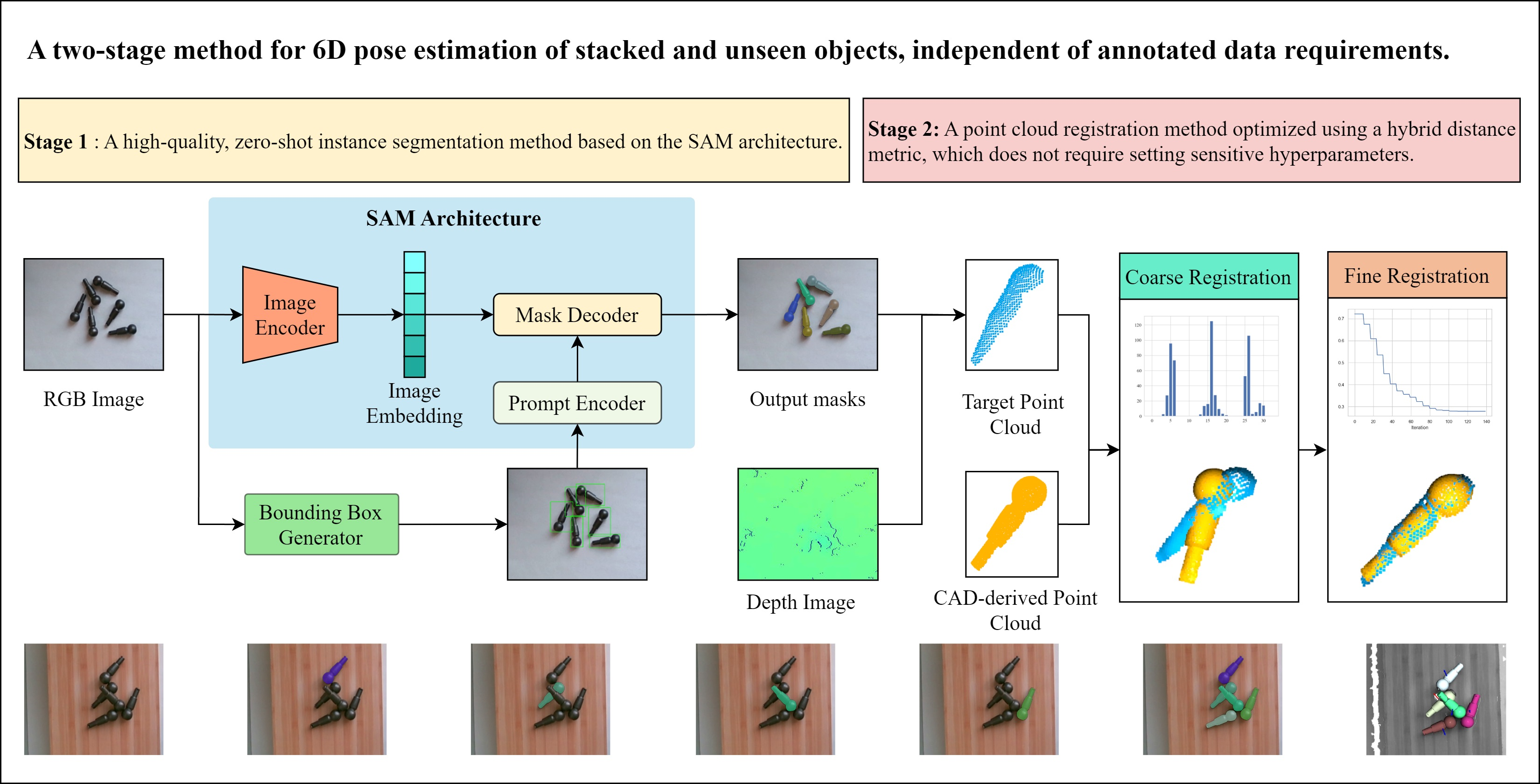
• A two-stage method for 6-DoF pose estimation of stacked and unknown objects, independent of annotated data requirements.
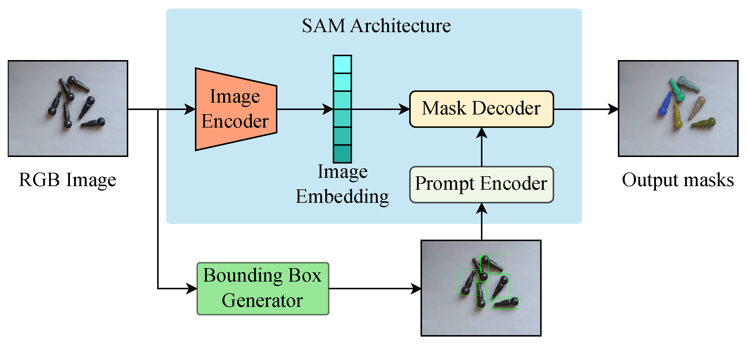
• A high-quality, zero-shot instance segmentation method based on the SAM architecture.
• A point cloud registration method optimized using a hybrid distance metric, which does not require setting sensitive hyperparameters.

2. Related Work

2.1. Pose Estimation with RGB-D Data

The 6-DoF object pose estimation based on RGB-D data uses images amalgamating color and depth information to precisely infer an object’s location and orientation in three-dimensional space. The DenseFusion framework [28] processes RGB and depth data through a heterogeneous structure, employing a dense fusion network strategy. It extracts dense feature embeddings at the pixel level, significantly enhancing the accuracy of object pose estimation. Building on this, He et al. introduced the Full Flow Bidirectional Fusion Network (FFB6D) [18], incorporating bidirectional fusion at various encoder–decoder layers to accommodate more complex scenes, particularly improving performance under occlusion and cluttered backgrounds. Diverging from methods that directly regress pose parameters, He et al.’s 3D keypoint voting network PVN3D [29] detects an object’s 3D keypoints through depth-based Hough voting and estimates the 6-DoF pose using the least squares method, a strategy crucial for robust keypoint detection. In the realm of category-level 6-DoF pose estimation, Wang et al. [30] devised a joint relation and cyclic reconstruction network strategy, delving into the intricate relationships between instance RGB images, point clouds, and category shape priors. Through iterative optimization, this approach precisely matches 3D models with observational data, offering innovative avenues for robotic manipulation and augmented reality technologies. Lin et al. employed a self-supervised Depth Prior Deformation Network (DPDN) [31] for estimating category-level 6-DoF object poses and dimensions to address the challenge of labeling data in practical applications. They focused on the transition from synthetic to real-world data, the so-called Sim2Real domain gap, achieving unsupervised domain adaptation through deformation feature matching with category shape priors. The 6IMPOSE framework [32], integrating a synthetic RGBD dataset generated by Blender with a target detection network based on YOLO-V4 and a lightweight pose estimation network, has propelled the advancement of real-time pose estimation. Despite these developments, 6-DoF object pose estimation based on RGB-D data still confronts numerous challenges. These include effectively integrating multimodal data, bridging the gap between synthetic and real data, enhancing robustness against occlusions and complex backgrounds, and achieving rapid and accurate real-time pose estimation. Additionally, newly introduced modules like the Depth Fusion Transformer (DFTr) [33] leverage cross-modal semantic associations to integrate globally enhanced features, offering fresh perspectives for resolving cross-modal feature fusion issues. In summary, while 6-DoF pose estimation with RGB-D imagery has made significant strides in technological breakthroughs and practical applications, further research and development are imperative for its widespread deployment in real-world applications.

2.2. Unseen Object Instance Segmentation

Accurately identifying and segmenting previously unseen objects is a complex yet crucial challenge. Back et al. [34] proposed a method that integrates synthetic data with RGB-D fusion technology within the Mask R-CNN framework, focusing on extracting shape information. They employed a domain randomization strategy to process textures, enhancing the algorithm’s adaptability to diverse environments. Innovatively, they also incorporated a confidence map estimator to utilize depth information effectively. UOAIS-Net [35], through its unique hierarchical occlusion modeling scheme, has significantly improved the recognition and segmentation of objects in complex environments, such as on desktops, indoors, and in trash bins, showing remarkable performance, especially in handling occlusions and cluttered backgrounds. This approach effectively deals with different parts of occluded objects, addressing a significant challenge in traditional object segmentation methods. Lu et al.’s work [36] combines multi-object tracking and video object segmentation techniques, offering a new perspective for robotic systems to handle unseen objects in dynamic environments. The key lies in generating segmentation masks through long-term interaction with objects and adapting to changes in object positions and environments in dynamic settings. “Side Adaptation Network” (SAN) [37] marks a significant open vocabulary semantic segmentation innovation. SAN achieves category recognition and segmentation by effectively integrating a frozen CLIP model, enhancing accuracy and network structural efficiency. Xiang et al.’s method [38] applies features from learned synthetic data to real-world images. Employing a metric learning loss function and mean shift clustering algorithm, their approach effectively distinguishes different objects at the pixel level, particularly in cluttered scenes. Xie et al. developed UOIS-Net [39], utilizing synthetic RGB-D data to effectively handle unseen object segmentation in desktop environments through a two-stage network architecture. Initially, the Depth Seeding Network (DSN) uses depth information to generate preliminary masks for object instances, followed by the Region Refinement Network (RRN) which refines these masks further by integrating RGB data. While these studies have achieved significant accomplishments in enhancing segmentation precision and dealing with complex environments, they still face challenges in practical applications, such as handling highly dynamic settings, extreme occlusions, or complex backgrounds. Most research remains limited to laboratory settings and synthetic data, and its generalizability to real-world environments requires further validation.

Recent advances in instance segmentation algorithms for unknown targets have been groundbreaking. The SAM, inspired by zero-shot learning from large language models, aims to develop a promptable, highly generalizable image segmentation model. SAM integrates a robust image encoder, a prompt encoder, and a lightweight mask decoder to achieve zero-shot transfer to new image distributions and tasks, often matching or surpassing fully supervised outcomes. The research team developed a data engine to enhance its generalizability, collaboratively creating the model and dataset with model-assisted dataset annotations. The resulting dataset, SA-1B, includes over one billion masks and eleven million images, characterized by high quality and diversity. SAM generates high-quality masks and handles various downstream tasks, including edge detection, object proposal generation, instance segmentation, and text-to-mask prediction. Recently, many scholars have researched and improved SAM from different perspectives. For instance, FastSAM [40] focuses on enhancing SAM’s operational speed for real-time applications. Zhang et al. developed MobileSAM [41] to reduce the model’s size, making it suitable for resource-limited mobile devices. Addressing the issue of SAM producing rough boundaries for complex structured objects, HQ-SAM [42] retains zero-shot capabilities while producing higher-quality masks. The instance segmentation model used in this article builds upon SAM, targeting optimization for issues like boundary blurriness, mask holes, and excessive segmentation of the same target in SAM, thereby elevating mask quality.

3. Materials and Methods

This paper introduces an innovative two-stage method, leveraging RGB-D data for object instance segmentation and 6-DoF pose estimation. Given an RGB-D image $I_{\mathrm{RGBD}}$ and the target CAD model $\left\{M_j\right\}$, our objective is to employ the color and depth information provided by each pixel of the RGB-D image, along with the three-dimensional point sets of the CAD models, to estimate the 6-DoF pose $\left\{P_j\right\}$ of each object within the image. Each pose $\left\{P_j\right\}$ comprises a rotation matrix $R_j\in \mathrm{SO}\left(3\right)$ and a translation vector $t_j\in {\mathbb{R}}^3$. We aim to ascertain an optimal set of $\left\{P_j\right\}$ that aligns each CAD model as closely as possible with its corresponding object in the RGB-D image.

The process of our method, as depicted in Figure 1, initiates with the first stage employing a zero-shot instance segmentation method based on the enhanced SAM model to discriminate and extract the mask of each component from the RGB image. Subsequently, we crop out the point clouds of the components from the depth map aligned with the RGB image. The second stage involves registering the cropped component point clouds with the point clouds derived from CAD, optimizing to attain the corresponding 6-DoF pose for each target. The methodologies of zero-shot instance segmentation and point cloud registration are expounded in detail in Section 3.1 and Section 3.2.

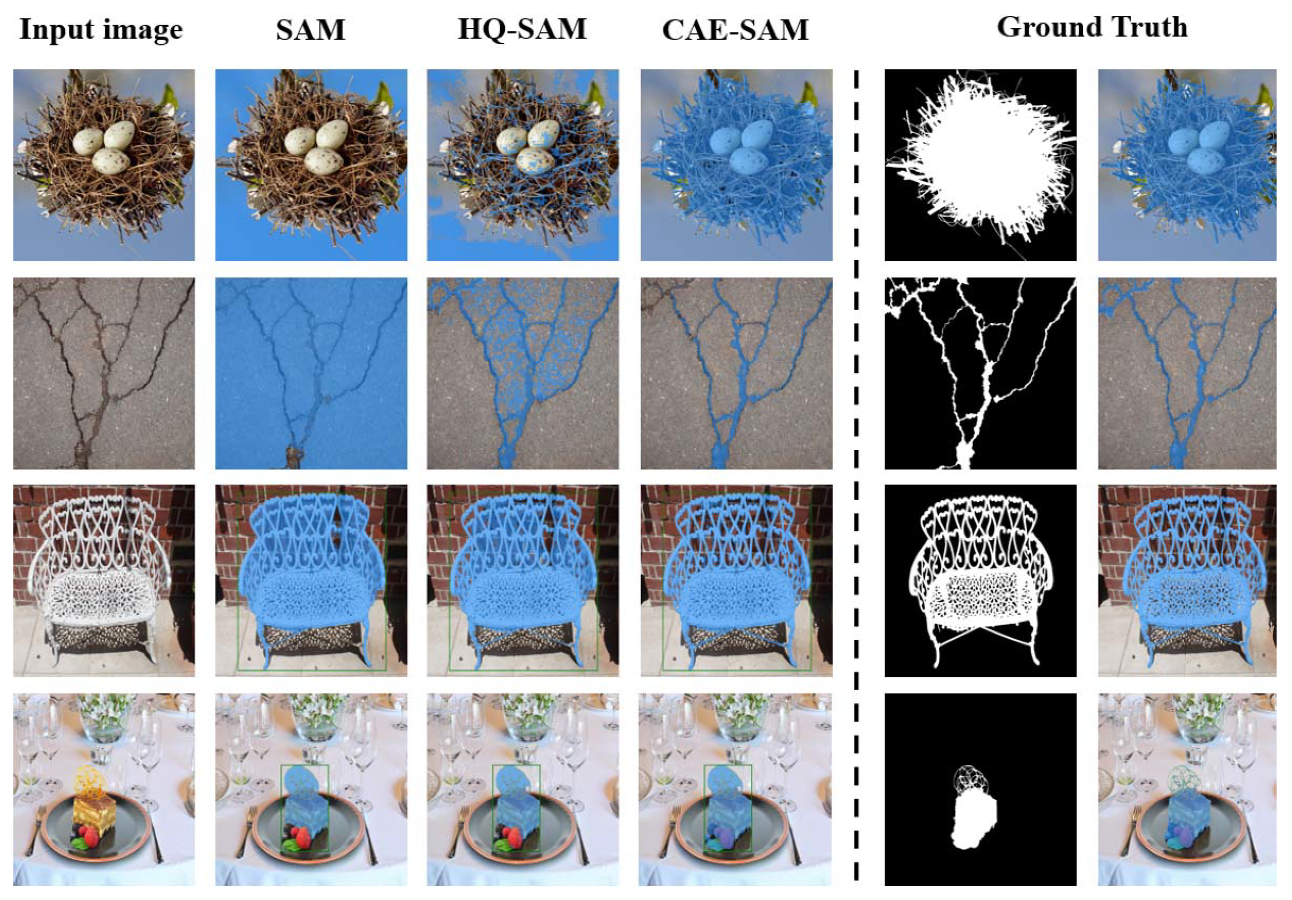
3.1. Context-Aware Enhanced SAM

The Context-Aware Enhanced SAM (CAE-SAM) method framework proposed in this paper is illustrated in Figure 2. We have meticulously integrated and repurposed the existing SAM structure to maintain the SAM’s prowess in zero-shot transfer. This approach aims to preserve the original model’s robust generalization capabilities while avoiding model overfitting or catastrophic forgetting that might result from direct fine-tuning of SAM. Specifically, our enhancements encompass three main aspects: Firstly, we have incorporated a convolutional neural network-based local spatial-feature-enhancement module within the image encoder. This module extracts local spatial context information from images, bolstering the model’s ability to handle image details and complex structures. Secondly, in the prompt encoder, we introduced global context tokens that engage in spatial dot-products with the fused global–local features, generating higher-quality masks. This enhancement elevates the model’s spatial understanding and segmentation precision. Lastly, we have implemented the Grounding-DINO [43] technique to generate target prompt boxes automatically, enhancing the model’s automation level and and segmentation accuracy.

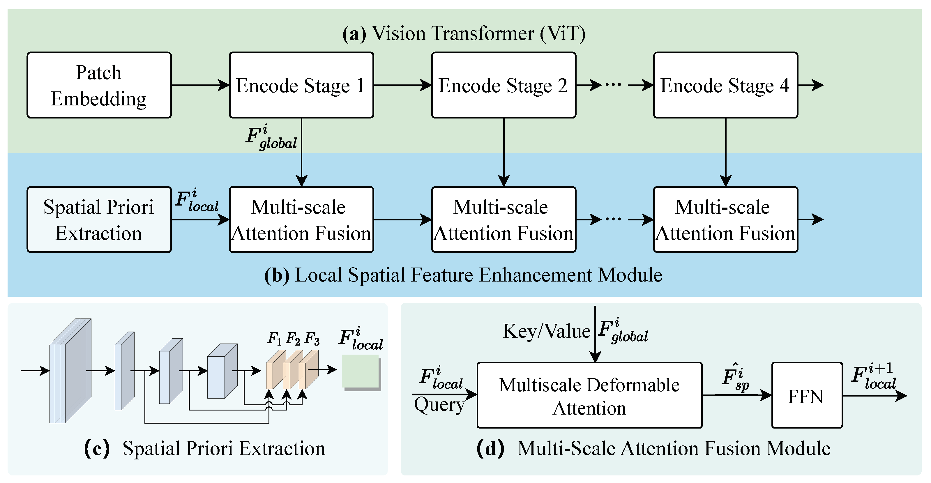
3.1.1. Image Encoder

Accurate segmentation necessitates image features endowed with a rich tapestry of global semantic context and intricate local boundary details. A Vision Transformer (ViT) [44] is employed as the image encoder in the original SAM. Thanks to its self-attention mechanism, ViT is adept at grasping the global context within images, decoding the intricate relationships among various image regions. This capability renders ViT particularly effective at interpreting the overall structure and relationships in images containing unknown information or novel targets, and ViTs pretrained on extensive datasets generally demonstrate superior generalization abilities. Despite ViT’s proficiency in understanding global structures, it may not capture local detail features as efficiently as CNNs, especially when processing images with subtle variations or obscure detail information. Inspired by recent research [45,46] indicating that convolution can enhance a Transformer’s ability to grasp local spatial information, and considering that the global information provided by ViT can direct CNNs to more precisely capture vital local features, this article combines CNN with ViT, forging a bidirectional complementary mechanism. Building on the original SAM decoder, a CNN-based spatial prior extractor is introduced to model the local spatial context of images, generating a feature pyramid that effectively supports dense prediction tasks. Then, in tandem with a multi-scale attention fusion module, the ViT features are leveraged further to fortify the local spatial attributes of the input images.

As depicted in Figure 3, the enhanced image encoder primarily comprises two components. The first is the foundational ViT encoder, consisting of an image block embedding layer and a sequence of Transformer encoders, as shown in Figure 3a. The second component is the novel local spatial-feature-enhancement module proposed in this paper, which includes (1) a spatial prior extraction module designed to model spatial contextual features from the input image and (2) a series of multi-scale attention fusion modules, purposed for merging and updating features across multiple scales, as illustrated in Figure 3b.

The input image is represented by a tensor X, with dimensions $B\times C\times H\times W$, where B, C, H, and W, respectively, signify the batch size, number of channels, height, and width. For the ViT encoder, the initial step involves passing X through an image block embedding layer, which segments the image into a series of non-overlapping blocks of size $16\times 16$. These blocks are subsequently flattened and mapped to a high-dimensional feature space of dimension D through a linear transformation, adjusting the feature dimensions to $B\times \frac{H}{16}\times \frac{W}{16}\times D$. Following this, these high-dimensional features are fused with corresponding positional encodings to introduce spatial location information. After that, the features undergo processing through L consecutive Transformer encoder layers, each incorporating self-attention mechanisms and feed-forward networks, thereby facilitating the extraction of single-scale features. To fully exploit the captured image information at various levels, the Transformer encoders of ViT are divided into N (where $N=4$) uniform encoding stages, each composed of $L/N$ encoder layers. For the i-th encoding stage, the output features are denoted as $F_{\mathrm{global}}^i\in {\mathbb{R}}^{(B\times \frac{HW}{{16}^2}\times D)}$.

The initial step for the local spatial-feature-enhancement module involves passing the input image X through the spatial prior extraction module, as depicted in Figure 3c. To maintain the richness of spatial information, this extractor adopts the backbone architecture of ResNet [47], employing a series of 3 × 3 convolutions with a stride of 2 to expand the number of channels while reducing the size of the feature map. Subsequently, a 1 × 1 convolution is used to project the feature map into a D-dimensional space. To accommodate the ViT model’s requirement for multi-scale information, we gather intermediate, varying-scale spatial features $\{F_1,F_2,F_3\}$ from this sub-network, where $F_1\in {\mathbb{R}}^{(B\times \frac{H}{8}\times \frac{W}{8}\times D)}$, $F_2\in {\mathbb{R}}^{(B\times \frac{H}{16}\times \frac{W}{16}\times D)}$, and $F_3\in {\mathbb{R}}^{(B\times \frac{H}{32}\times \frac{W}{32}\times D)}$. Finally, to merge these multi-scale spatial features, we flatten and concatenate the resulting feature sets along the channel dimension, forming a comprehensive local spatial prior $F_{\mathrm{local}}^1\in {\mathbb{R}}^{(B\times (\frac{HW}{8^2}+\frac{HW}{{16}^2}+\frac{HW}{{32}^2})\times D)}$, which is then inputted into subsequent multi-scale attention fusion modules.

Further, N sparse attention and feed-forward networks are used to update the spatial features $F_{\mathrm{sp}}^i$, with the generated $F_{\mathrm{sp}}^{(i+1)}$ serving as the input for the next multi-scale feature fusion module, as shown in Figure 3d. Here, the sparse attention employs multi-scale deformable attention operations, aiming to enhance the model’s sensitivity to multi-scale information without increasing computational complexity. The process can be formulated as:

$$\begin{array}{cc}\hfill & {\widehat{F}}_{\mathrm{local}}^i=F_{\mathrm{local}}^i+\mathrm{Attention}(\mathrm{norm}\left(F_{\mathrm{local}}^i\right),\mathrm{norm}\left(F_{\mathrm{global}}^{(i+1)}\right)),\hfill \\ \hfill & F_{\mathrm{local}}^{(i+1)}={\widehat{F}}_{\mathrm{local}}^i+\mathrm{FFN}\left(\mathrm{norm}\left({\widehat{F}}_{\mathrm{sp}}^i\right)\right),\hfill \end{array}$$

(1)

where $F_{\mathrm{global}}^i$ and $F_{\mathrm{local}}^i$ together serve as the input for the i-th multi-scale feature fusion module. $F_{\mathrm{global}}^i\in {\mathbb{R}}^{(B\times \frac{HW}{{16}^2}\times D)}$ acts as the key and value vectors, while $F_{\mathrm{local}}^i\in {\mathbb{R}}^{(B\times (\frac{HW}{8^2}+\frac{HW}{{16}^2}+\frac{HW}{{32}^2})\times D)}$ serves as the query vector. This combination ensures that each step of feature updating is based on current and higher-level information, enhancing the model’s capability to handle size variations and complex details. In Equation (1), $\mathrm{Attention}(·)$ denotes multi-scale deformable attention, and $\mathrm{norm}(·)$ represents LayerNorm used for normalizing features, providing a uniform input for the attention layer and subsequent feed-forward network (FFN), thereby ensuring the stability and efficacy of feature updates.

Finally, this paper merges the output features $F_{\mathrm{global}}^i$ from each stage of the ViT with the final $F_{\mathrm{local}}^i$ obtained from the local spatial-feature-enhancement module. This integration produces a multi-scale encoded result from the image encoder. This multi-scale encoded result is then further combined with the mask features in the subsequent SAM’s mask decoder, culminating in a global–local feature set used for mask prediction.

3.1.2. Global Context Token

To correct mask errors in the SAM output and fully leverage the local spatial features extracted by the local spatial-feature-enhancement module, a global context token and a new mask prediction layer are introduced for high-quality mask prediction. This paper reuses and fixes SAM’s mask decoder, introducing a new learnable global context token $T_{\mathrm{gc}}\in {\mathbb{R}}^{(1\times 256)}$, which is concatenated with SAM’s output token $T_{\mathrm{o}}\in {\mathbb{R}}^{(4\times 256)}$ and prompt token $T_{\mathrm{p}}\in {\mathbb{R}}^{(N_{\mathrm{prompt}}\times 256)}$. The concatenated result $T_{\mathrm{a}}\in {\mathbb{R}}^{(1+4+N_{\mathrm{prompt}})\times 256}$ serves as the input to SAM’s mask decoder. Similar to the original output token computation process, the global context token first undergoes self-attention with other tokens, followed by bidirectional cross-attention with the image to update its features. After passing through two decoder layers, global image information contained in the global context token, critical geometric information in the prompt token, and hidden mask information in the output token are obtained. Finally, a new Multilayer Perceptron (MLP) is added to generate dynamic weights from the updated global context token, which are then spatially dotted with the global–local features to produce high-quality masks.

3.1.3. Bounding Box Generator

The original SAM model utilizes 32 × 32 pixel points as prompt tokens for the “segment anything” mode, which encounters several issues in practical applications. Firstly, point prompts may lead the model to over-focus on local details while neglecting the overall context of the target. This can result in excessive segmentation, mistakenly dividing a single target into multiple regions, as illustrated in Figure 4. Moreover, this approach might incorrectly classify background pixels as part of the target, especially in situations lacking sufficient segmentation information. These limitations impact the accuracy of segmentation and may also reduce the model’s generalizability across targets of varying sizes and complexities.

To overcome these segmentation challenges, this paper introduces a bounding box generator based on Grounding DINO. Trained through self-supervised learning, Grounding DINO can understand and locate targets in images from textual descriptions, generating precise candidate frames for targets. These candidate frames, used as inputs for the prompt encoder, serve as segmentation cues, assisting the model in differentiating foreground targets from the background. Consequently, this reduces the misclassified background pixels in segmentation, enhancing overall accuracy. With this improvement, the CAE-SAM model is more effectively equipped to handle complex visual scenes, thereby elevating the performance of image segmentation tasks.

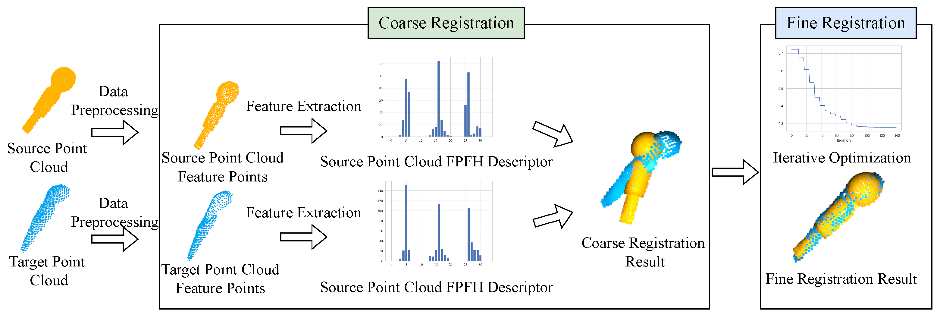
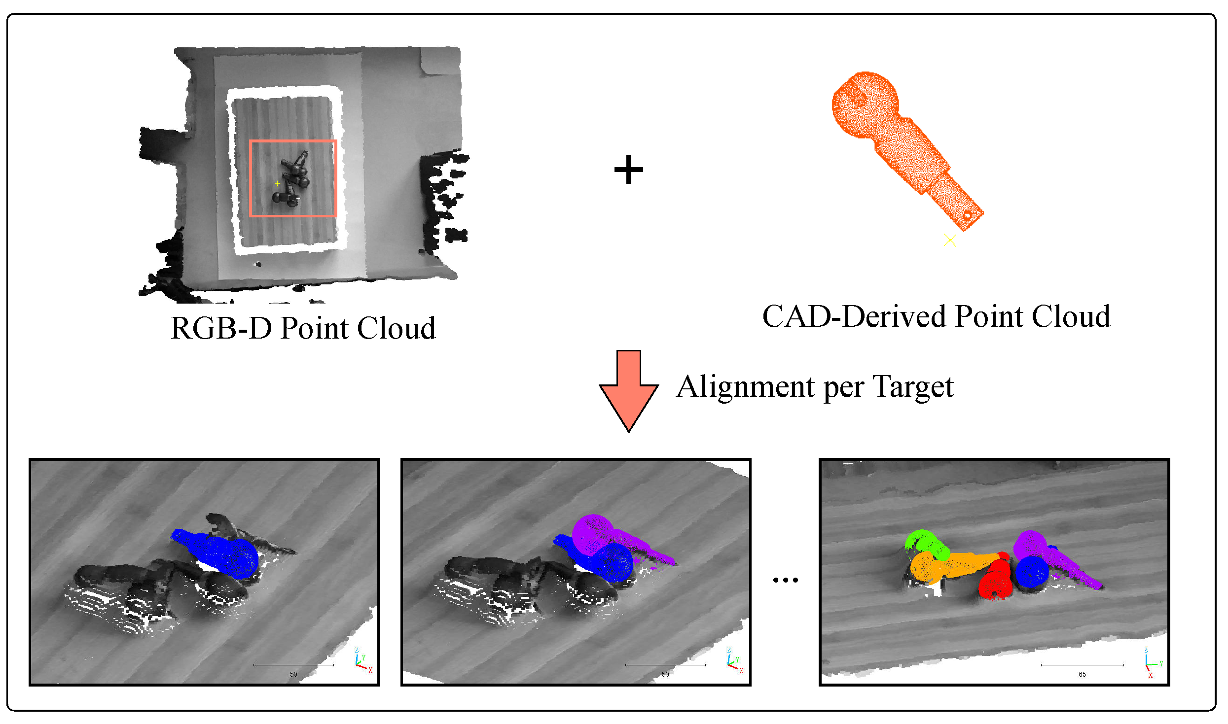
3.2. Point Cloud Registration

Deep learning-based point cloud registration methods utilize intricate neural network architectures to learn and extract deep features from data autonomously. They are adept at processing point clouds with complex geometric structures and maintain stability in environments with high noise levels and data heterogeneity. However, the effectiveness of these methods is highly contingent on the quality and diversity of the training data and typically requires significant computational resources for model training and optimization. Additionally, many deep learning-based point cloud registration methods still rely on traditional optimization techniques like the ICP algorithm for final fine-tuning and optimization after achieving preliminary registration. Thus, traditional point cloud methods continue to play a vital role in point cloud registration tasks.

Considering that traditional methods are generally easier to deploy and maintain, and their updates and iterations are more straightforward, requiring less frequent model retraining when data distributions change, this paper follows the thought process of traditional point cloud registration methods, as illustrated in Figure 5. Initially, the source and target point clouds undergo preprocessing to extract key feature points. Subsequently, in the coarse registration phase, feature histograms are used to describe each feature point. These features facilitate the preliminary alignment of the source point cloud with the target point cloud, resulting in a roughly matched point cloud. Finally, based on the coarse registration, this paper proposes a point cloud registration method optimized using a hybrid distance metric to achieve fine registration of the point clouds.

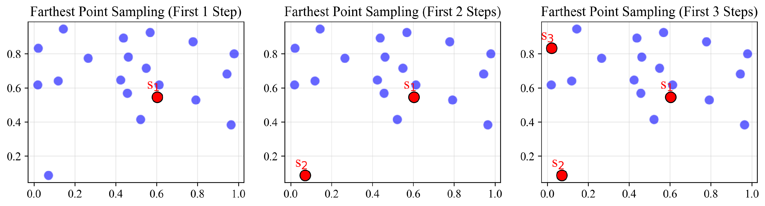
3.2.1. Data Preprocessing

In point cloud preprocessing, we primarily perform point cloud downsampling. Given a point cloud set $P=\{p_1,p_2,\dots ,p_n\}$ comprising n points, we select m representative points, resulting in a sampled subset $S=\{s_1,s_2,\dots ,s_m\}$. Inspired by the approach of PointNet++ [25], we employed the Farthest Point Sampling (FPS) [48] algorithm for point cloud downsampling. This algorithm iteratively selects the farthest point from the existing sampled point set as the new sample point, ensuring uniform distribution and broad coverage of the sample points across the dataset, thereby enhancing the representativeness of the sampled set. Secondly, its algorithmic simplicity makes FPS easy to implement and integrate into various data processing workflows, offering adaptability and flexibility. An illustrative diagram of the FPS algorithm execution is shown in Figure 6, with red points representing the chosen sample points. The steps of the FPS algorithm are as follows:

• Randomly select an initial point from the dataset as the first sample point.
• Compute the Euclidean distance from each point in the dataset to the already selected sample points, providing necessary distance information for selecting the next sample point.
• In each iteration round, select the point with the maximum distance to the nearest point in the current sample point set as the new sample point. This selection process is based on the farthest point criterion, aimed at maximizing the distance between the new sample point and the existing sample point set.
• After each new sample point selection, update the shortest distance from each point in the dataset to the nearest sample point, ensuring that the most representative point relative to the current sample point set is chosen in each iteration.
• Repeat the above iteration process until the predetermined number of sample points is reached or other stopping criteria are met.

For the target objects in this paper, Figure 7 illustrates the effect of the FPS algorithm in point cloud downsampling. The figure includes the original point cloud and the downsampling results at four different sampling rates (80%, 60%, 40%, and 20%). It can be observed from the figure that the FPS algorithm can effectively retain the critical structural features of the point cloud even at lower sampling rates. As the sampling rate decreases, the number of points reduces, but the main shape and structure of the original point cloud are still discernible.

3.2.2. Point Cloud Feature Extraction

The 3D point cloud feature extraction aims to precisely extract geometric and topological critical features from the extensive point cloud data, providing the necessary information foundation for registration. This paper selects the Fast Point Feature Histogram (FPFH) method for feature extraction due to its significant advantages in processing efficiency, robustness, adaptability, and rotational invariance. FPFH dramatically enhances the efficiency of feature extraction through a simplified computation process and demonstrates robust performance when dealing with noisy or unevenly sampled point cloud data. Moreover, it adapts well to point clouds of varying densities and possesses rotational invariance, which is crucial for point cloud registration in the real world with varying viewpoints.

The core steps in calculating the point cloud feature descriptors using FPFH [49] mainly include defining a local coordinate system and feature extraction. Initially, for each point p in the point cloud $P=\{p_1,p_2,\dots ,p_n\}$, its neighborhood point set $N_p$ is determined, usually comprising all points within a certain neighborhood radius r. To enhance the adaptability and robustness of the FPFH algorithm in processing point clouds of different densities and distributions, we adopt a neighborhood radius strategy adaptive to the local density of the point cloud. This strategy allows the neighborhood radius to automatically adjust according to the actual local density of the point cloud, thereby more effectively capturing local features in noisy or unevenly sampled point clouds. By reducing the need for manual parameter tuning, this adaptive neighborhood radius strategy not only improves user-friendliness but also helps more accurately describe the point cloud’s local structural information. Specifically, the radius calculation formula is defined as follows:

$$r=k\frac{1}{n}\sum _{i=1}^n\underset{p_j\in P,j\ne i}{min}{∥p_j-p_i∥}_2,$$

(2)

where k is a scaling factor, which can be varied to control the size of the neighborhood, adapting to different characteristics of point cloud data. It represents the statistical Euclidean distance between a sample point $p_i$ and its nearest point $p_j$ in the point cloud P.

Further, for each point p in the point cloud and its neighboring points, a local coordinate system is constructed, as shown in Figure 8. The UVW coordinate system is defined as follows:

$$\begin{array}{cc}\hfill u& =n_{P_c},\hfill \\ \hfill v& =\frac{P_n-P_c}{\parallel P_n-P_c{\parallel }_2}\times u,\hfill \\ \hfill w& =u\times v,\hfill \end{array}$$

(3)

where $n_{P_c}$ is the normal vector of the point $P_c$. Based on the UVW coordinate system, the Simplified Point Feature Histograms (SPFHs) for each point are calculated by computing the angular variations of the normal vectors of points $P_c$ and $P_n$ in the local coordinate system. This typically includes three key angles:

$$\begin{array}{cc}\hfill \alpha & =vs.·n_{P_n},\hfill \\ \hfill \varphi & =u·\frac{P_n-P_c}{\parallel P_n-P_c{\parallel }_2},\hfill \\ \hfill \theta & =arctan(w·n_{P_n},u·n_{P_n}),\hfill \end{array}$$

(4)

These angles describe the local surface geometry of the point. Subsequently, these angular values are used to update the SPFH of the point. Next, the FPFH feature of point $P_c$ is generated by weighted averaging of its own SPFH with the SPFH features of its neighboring points, as indicated in Equation (5). This weighted averaging approach takes into account the distances between neighboring points, allowing for a broader capture of local geometric features.

$$\mathrm{FPFH}\left(P_c\right)=\mathrm{SPFH}\left(P_c\right)+\frac{1}{n}\sum _{i=1}^n\frac{1}{\parallel P_n-P_c{\parallel }_2}\times \mathrm{SPFH}\left(P_n\right),$$

(5)

where n is the number of points in the neighborhood of $P_c$.

3.2.3. Point Cloud Coarse Registration

Point cloud coarse registration involves aligning two point cloud datasets at a macro level, providing an approximately correct starting point for fine registration. This is particularly effective when there is a significant initial discrepancy between the source and target point clouds, as it enables the identification and matching of similar regions in different point clouds, thus achieving preliminary alignment of the two point clouds. This paper employs the Fast Global Registration (FGR) algorithm [50] for the coarse registration of the source point cloud P and the target point cloud Q. Initially, the FPFH features of each point in the two point clouds are constructed, represented as $F\left(P\right)=\left\{F\right(p):p\in P\}$ and $F\left(Q\right)=\left\{F\right(q):q\in Q\}$. Then, correspondences between point pairs are established based on Equation (6), and these correspondences are not recalculated throughout the optimization process.

$$(p,q)=\underset{(p,q)}{arg\; min}{\parallel F\left(p_i\right)-F\left(q_i\right)\parallel }_2,$$

(6)

That is, for each point p in point set P, find the nearest neighbor feature $F\left(q\right)$ in point set Q, and vice versa. Further, the objective function for optimization is defined as follows:

$$E\left(T\right)=\sum _{(p,q)\in K}{\rho (\parallel q-Tp\parallel }_2),$$

(7)

where $E\left(T\right)$ represents the total distance after optimization, K is the set formed by point pairs $(p,q)$, T is the rigid transformation to be solved, and $\rho$ is a robust penalty function, employing the scaled Geman–McClure function. This function is used to minimize the distance between corresponding points while automatically weakening the impact of incorrect matches, as defined in Equation (8). The optimization goal is to adjust the transformation T such that the value of the objective function $E\left(T\right)$ is minimized, thereby achieving optimal alignment between point sets P and Q.

$$\rho \left(x\right)=\frac{\mu x^2}{\mu +x^2},$$

(8)

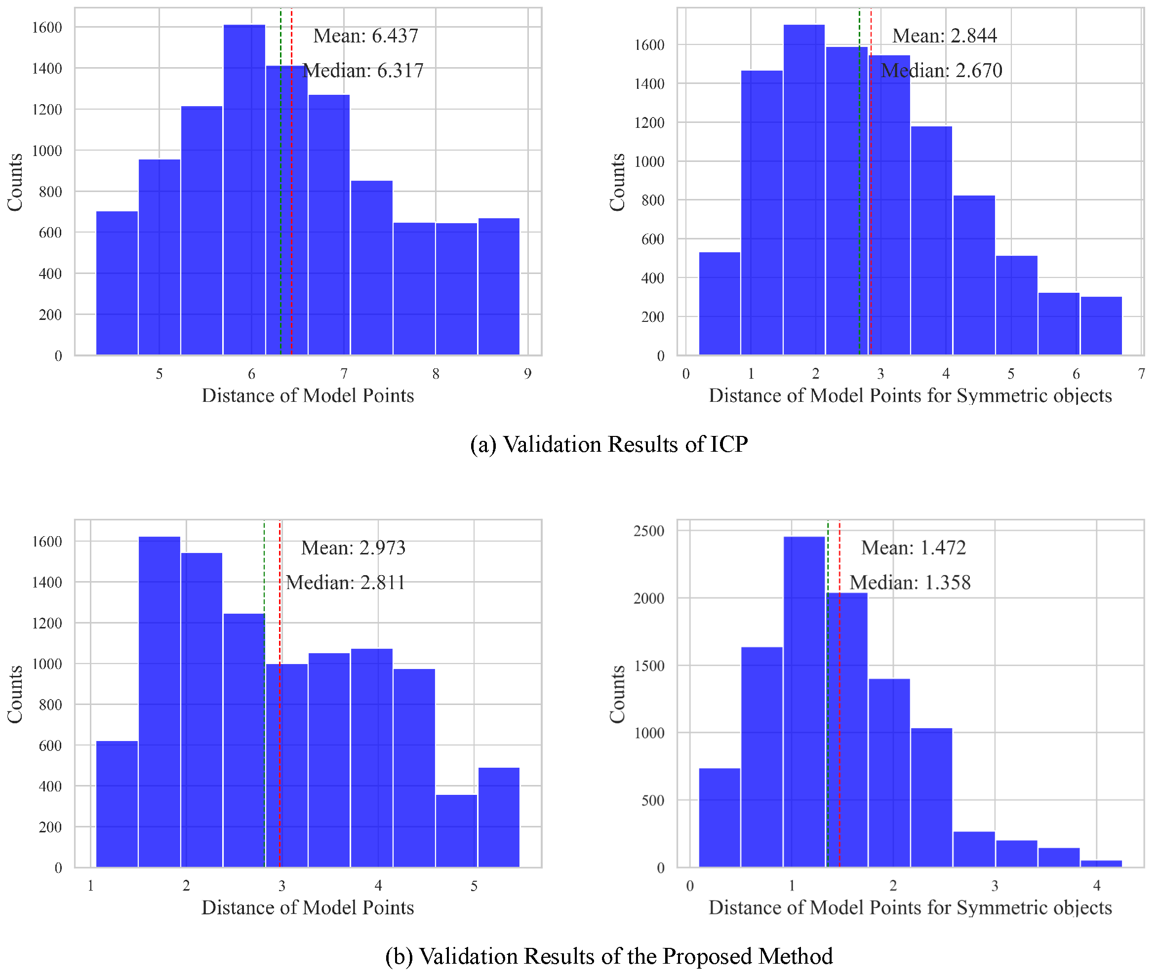
3.2.4. Point Cloud Fine Registration

The ICP algorithm holds a central position in traditional point cloud fine registration due to its efficiency, simplicity, broad application scope, and time-tested stability. The maximum correspondence distance is a crucial parameter in the ICP algorithm, defining the maximum allowable distance between point pairs considered during the search for nearest-point correspondences. The ICP algorithm identifies the nearest point in Q for each point in P during each iteration. If $p_i$ is a point in P and $q_i$ is the nearest point to $p_i$ in Q, then the maximum correspondence distance $d_{\max }$ is used to filter the point pair $(p_i,q_i)$. If $\mathrm{distance}(p_i,q_i)\le d_{\max }$, then $(p_i,q_i)$ is considered a valid corresponding point pair; otherwise, the pair is not considered for registration computation. Therefore, setting the maximum correspondence distance impacts the performance of the ICP algorithm. Setting the distance threshold too high may cause the algorithm to consider distant point pairs as correspondences, introducing erroneous matches and leading to a result that deviates from the true value. Furthermore, including more potentially irrelevant point pairs may make the results unstable. Erroneous matches could also interfere with the algorithm’s convergence process, leading to convergence to an incorrect configuration or even failure to converge in some cases. Conversely, setting the threshold too low might exclude many point pairs that should match, potentially requiring more iterations for the algorithm to achieve a satisfactory registration result, or it may not reach an ideal registration state. Additionally, a more restrictive threshold might easily cause the algorithm to become trapped in local optima. Figure 9 demonstrates the situations where an incorrect setting of the maximum correspondence distance leads to non-convergence of the algorithm and trapping in local optima.

To address the issues above and improve the registration accuracy and robustness of the algorithm, we propose a point cloud registration method optimized based on a hybrid distance measure. This method eliminates the need to set sensitive hyperparameters like the maximum correspondence distance, offering a more flexible and accurate approach to processing point cloud data.

Finding the Nearest Point. To organize point $q_j$ for rapid retrieval, a KD-tree of the target point cloud Q is constructed. For each point $p_i$ in point cloud P, the nearest point $q_{\mathrm{nearest}\left(i\right)}$ in Q in terms of Euclidean distance is found in the KD-tree, represented as follows:

$$q_{\mathrm{nearest}\left(i\right)}=\underset{q_j\in Q}{arg\; min}{\parallel p_i-q_j\parallel }_2.$$

(9)

Hybrid Distance Measure Calculation. The hybrid distance measure combines point-to-point and point-to-plane distances. Given a set of transformation parameters $\theta$ and weight parameter $\alpha$, the hybrid distance from P to Q is computed as follows:

$$D(p_i,\theta ,\alpha )=\alpha d_{\mathrm{pt}-\mathrm{pt}}(p_i,\theta )+(1-\alpha )d_{\mathrm{pt}-\mathrm{pl}}(p_i,\theta ),$$

(10)

where $d_{\mathrm{pt}-\mathrm{pt}}(p_i,\theta )$ is the point-to-point distance, defined as follows:

$$d_{\mathrm{pt}-\mathrm{pt}}(p_i,\theta )={\parallel T\left(\theta \right)p_i-q_{\mathrm{nearest}\left(i\right)}\parallel }_2.$$

(11)

$d_{\mathrm{pt}-\mathrm{pl}}(p_i,\theta )$ is the point-to-plane distance, defined as follows:

$$d_{\mathrm{pt}-\mathrm{pl}}(p_i,\theta )=|(T\left(\theta \right)p_i-q_{\mathrm{nearest}\left(i\right)})·n_{\mathrm{nearest}\left(i\right)}|,$$

(12)

where $\alpha$ is a learnable parameter used to balance the weights of the two types of distances. $T\left(\theta \right)$ is the transformation matrix defined according to the set of transformation parameters $\theta$.

To reduce the sensitivity of the hybrid distance measure to extreme outliers and to improve numerical stability during the optimization process, we introduce the Huber loss, defined as follows:

$$L\left(r\right)=\left\{\begin{array}{cc}\frac{1}{2}{r}^2,\hfill & \mathrm{if}\left|r\right|\le \delta \hfill \\ \delta \left(\right|r|-\frac{1}{2}\delta ),\hfill & \mathrm{otherwise}\hfill \end{array}\right.$$

(13)

where r is the residual, and $\delta$ is a threshold. In this paper, the transformation parameters $\theta$ and the weight parameter $\alpha$ are optimized by minimizing the total hybrid distance, with the optimization problem formulated as follows:

$$\underset{\theta ,\alpha }{min}\sum _{i=1}^{\left|P\right|}L\left(D(p_i,\theta ,\alpha )\right),$$

(14)

where $\left|P\right|$ denotes the total number of points in the point cloud P.

To solve this problem, we employed the Levenberg–Marquardt (LM) algorithm, a widely used nonlinear minimization method suitable for solving large-scale nonlinear least-squares problems. In each iteration, the LM algorithm updates $\theta$ and $\alpha$ by solving Equation (15).

$$(J^{T}J+\lambda \mathrm{diag}\left(J^{T}J\right))\mathsf{\Delta }=-J^{T}r,$$

(15)

where J is the Jacobian matrix of the objective function, $\mathsf{\Delta }$ represents the step length of the parameter update, r is the residual vector, and $\lambda$ is a tuning parameter, controlling whether the algorithm leans more towards gradient descent or the Gauss–Newton method. If the residual decreases, $\lambda$ is increased; otherwise, it is decreased. Based on the definition above, we know that

$$r_i(\theta ,\alpha )=L\left(D(p_i,\theta ,\alpha )\right)$$

The Jacobian matrix J is defined as follows:

$$J=\left[\begin{array}{cccc}\frac{\partial r_1}{\partial {\theta }_{{\mathrm{rot}}_1}}& \cdots & \frac{\partial r_1}{\partial {\theta }_{{\mathrm{trans}}_3}}& \frac{\partial r_1}{\partial \alpha }\\ ⋮& \ddots & ⋮& ⋮\\ \frac{\partial r_n}{\partial {\theta }_{{\mathrm{rot}}_1}}& \cdots & \frac{\partial r_n}{\partial {\theta }_{{\mathrm{trans}}_3}}& \frac{\partial r_n}{\partial \alpha }\end{array}\right]$$

Finally, the optimal set of parameters, including the transformation parameters $\theta$ (comprising rotation and translation parameters) and the hybrid weight parameter $\alpha$, is obtained through iterative optimization.

4. Results

In Section 4, we conducted evaluations of the zero-shot instance segmentation algorithm CAE-SAM and the point cloud registration-based target 6-DoF pose estimation.

4.1. CAE-SAM Experimental Results and Analysis

Dataset. The instance segmentation in this paper was trained and evaluated on the HQSeg-44K dataset. This dataset amalgamates six high-quality image datasets, encompassing over 1000 diverse semantic categories. It includes 44,359 images for training and 1537 images for testing.

Training Details. During the training process, we adopted a strategy of keeping the pretrained SAM model parameters unchanged while updating parameters solely in the local spatial-feature-enhancement module, Global Context Tokens, and their associated three-layer MLP, as well as in the convolutional layers used for fusing global and local features. Additionally, the bounding box generator based on Grounding DINO was utilized in the point cloud registration inference process but was not involved in the training stage. Gaussian noise and large-scale jitter techniques were introduced to augment the data to enhance dataset diversity. Random noise was introduced in the real mask’s edge areas to simulate imperfect edge scenarios that might occur in the real world. Large-scale jitter technology was employed for random scaling of images, aiding the model in better adapting to objects of varying sizes. The model was trained using the Adam optimizer, with an initial learning rate of 0.001, and the StepLR strategy was used to reduce the learning rate every 5 epochs, with a total of 14 epochs in the training process.

Validation Metrics. To comprehensively assess the performance of the proposed CAE-SAM model, two key metrics were used, mask Intersection over Union (mIOU) [31,37,38] and boundary Intersection over Union (mBIOU) [42,51], to evaluate the improvement in mask quality quantitatively. mIOU is a widely applied mask-based segmentation metric in semantic, instance, and panoramic segmentation tasks and dataset evaluations. It is assessed by calculating the area intersection over the union between two masks. However, as mIOU treats all pixels equally, it reduces sensitivity in assessing the boundary quality of larger objects. Therefore, to evaluate the quality of boundary segmentation more precisely, the mBIOU metric was introduced. mBIOU focuses on assessing the segmentation performance of boundary regions and can more intricately reflect the model’s capability in handling edge details. The specific formulas for these metrics are as follows:

$$mIoU=\frac{1}{N}\sum _{i=1}^N\frac{|G_i\cap P_i|}{|G_i\cup P_i|},$$

(16)

$$mBIoU=\frac{1}{N}\sum _{i=1}^N\frac{|(G_{id}\cap G_i)\cap (P_{id}\cap P_i)|}{|(G_{id}\cap G_i)\cup (P_{id}\cap P_i)|},$$

(17)

where N represents the number of images, $G_i$ is the true mask region of the i-th image, $P_i$ is the predicted mask region of the i-th image, $G_{id}$ is the true boundary mask region of the i-th image, $P_{id}$ is the predicted boundary mask region of the i-th image, and d is the pixel width of the boundary region.

In this paper, comparative tests were conducted on SAM, HQ-SAM, and CAE-SAM models across four test subsets of the HQSeg-44K dataset (DIS, COIFT, HRSOD, ThinObject), with quantitative results presented in

Table 1. Comparison of SAM, HQ-SAM, and CAE-SAM models on DIS, COIFT, HRSOD, and ThinObject test sets, evaluated using the metrics of mIoU and mBIoU.

Model	DIS		COIFT		HRSOD		ThinObject		Average
	mIoU	mBIoU	mIoU	mBIoU	mIoU	mBIoU	mIoU	mBIoU	mIoU	mBIoU
SAM	0.620	0.528	0.921	0.865	0.902	0.831	0.736	0.618	0.795	0.711
HQ-SAM	0.786	0.704	0.948	0.901	0.936	0.869	0.895	0.799	0.891	0.818
CAE-SAM	0.813	0.733	0.956	0.913	0.946	0.891	0.934	0.845	0.912	0.846

. The CAE-SAM model demonstrated superior performance in all test sets. Specifically, regarding the mIoU metric, the CAE-SAM model performed markedly better than both SAM and HQ-SAM across all test sets. Compared to the SAM model, the HQ-SAM showed average gains of 0.096 and 0.107 in mIoU and mBIoU metrics, respectively. However, the gains of the CAE-SAM model relative to the SAM model were even more significant, reaching 0.117 and 0.135, respectively. This substantial improvement underscores CAE-SAM’s leading position in overall performance and reflects its significant advancements in mask accuracy and edge segmentation quality. Additionally, the consistency of the CAE-SAM model across different datasets demonstrates its robust generalization ability for various image types. Its performance in the ThinObject test set is particularly noteworthy. CAE-SAM achieved a mIoU score of 0.934, significantly surpassing both SAM and HQ-SAM models and showcasing its exceptional capability in handling delicate and complex objects. Similarly, on the mBIoU metric, CAE-SAM reached 0.845 in the ThinObject test set, highlighting the model’s precision in boundary detail processing.

Figure 10 displays qualitative experimental results of the SAM, HQ-SAM, and CAE-SAM models on the HQSeg-44K dataset and their segmentation ground truths. From the first and second images in the figure, it can be seen that in scenarios where the foreground object occupies a more significant proportion of the image area, SAM and HQ-SAM, which solely utilize ViT for extracting image encoding features, may not adequately capture all local information of the target instance due to ViT’s fixed-size image blocks. This limitation could result in the final segmentation results focusing more on the background areas and overlooking the foreground object. On the other hand, the third image demonstrates the CAE-SAM model proposed in this paper, exhibiting higher finesse in segmenting local edge details. Furthermore, the fourth image reveals deficiencies in SAM and HQ-SAM’s handling of the overall integrity of targets within prompt boxes. In contrast, the CAE-SAM model proposed in this paper shows superior segmentation performance, even when there is significant color variation among different target parts.

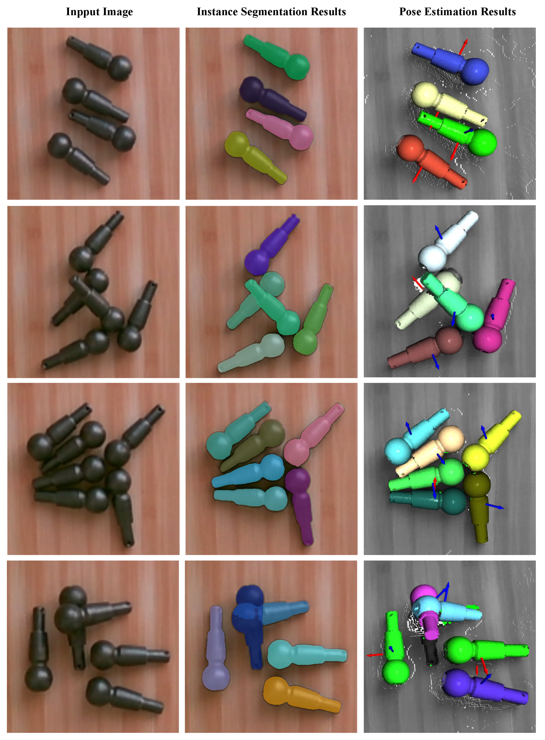
4.2. Pose Estimation Experimental Results and Analysis

Experimental Configuration. The inference process of the CAE-SAM instance segmentation method and the subsequent target 6-DoF pose estimation based on segmentation results were both executed on a host equipped with an Intel(R) Core(TM) i5-12490F and NVIDIA GeForce RTX 3060. In the 6-DoF pose estimation, the point cloud fine registration component, utilizing a point cloud registration method optimized by a hybrid distance measure, obviates the need for setting hyperparameters. Key parameter settings include the normal estimation radius, FPFH feature estimation radius, and the FGR algorithm distance threshold. These three hyperparameters were set based on the average distance radius from Equation (2), respectively, set to $3r$, $5r$, and $3r$. Additionally, the maximum number of iterations for the FGR algorithm was set to 20, and the maximum number of corresponding points was set to the quantity of the target point cloud. The number of points sampled from the CAD-derived point cloud was set to 10,000.

Dataset. To comprehensively evaluate the point cloud registration method, this paper constructed a high-quality test dataset using CloudCompare software (v2.13.alpha), comprising 100 sets of workpieces, covering various states of the workpieces, such as laid flat and stacked. To ensure data accuracy, Aruco markers were avoided in determining target poses. The dataset construction involved two main steps: First, color and depth images of the workpieces were captured using a Intel RealSense D455 camera, with the image resolution set to 1280 × 720. Further, leveraging the camera’s intrinsic parameters, RGB-D point clouds were generated and imported into CloudCompare. Secondly, in CloudCompare, we manually aligned CAD-derived point clouds to the positions of the workpieces in the RGB-D point clouds, matching the actual locations of the workpieces in the images. Specifically, annotated examples are illustrated in Figure 11.

Evaluation Metrics. In this section, we employ two metrics, ADD (Average Distance of Model Points) and ADD-S (Average Distance of Model Points for Symmetric objects) [18,29,32,33] to assess the accuracy of 6-DoF pose estimation. The ADD metric quantifies the average Euclidean distance between corresponding points in the point cloud under the actual and predicted poses, calculating the mean discrepancy of each point’s transformed location in the point cloud. On the other hand, given the rotational symmetry of the target workpieces in this study, we also utilize the ADD-S metric, designed explicitly for symmetric objects. As symmetric objects can have multiple visually indistinguishable valid poses, ADD-S computes the mean of the shortest distances between all possible corresponding points under the predicted pose and the actual pose points. The formulas for calculating ADD and ADD-S are as follows:

$$\begin{array}{cc}\hfill & \mathrm{ADD}=\frac{1}{m}\sum _{v\in V}{∥(Rv+T)-(R^{\prime }v+T^{\prime })∥}_2\hfill \end{array}$$

(18)

$$\begin{array}{cc}\hfill & \mathrm{ADD}-\mathrm{S}=\frac{1}{m}\sum _{v_1\in V}\underset{v_2\in V}{min}{∥(R{v}_1+T)-(R^{\prime }{v}_2+T^{\prime })∥}_2\hfill \end{array}$$

(19)

where m is the number of points in the CAD-derived point cloud V, R and T, respectively, represent the rotation and translation matrices of the actual pose, $R^{\prime }$ and $T^{\prime }$, respectively, represent the rotation and translation matrices of the predicted pose, and $v_1$ and $v_2$, respectively, represent the closest points under the actual and predicted poses.

Given that current deep learning-based 6-DoF pose estimation algorithms necessitate tuning on datasets, we streamlined our operations by solely comparing our results with the optimized ICP algorithm available in Open3D, employing the CAE-SAM proposed in this paper for target segmentation. During the computation of ADD and ADD-S metrics, we tallied the number of points across various distance scales, as depicted in Figure 12. The verification results of the ICP algorithm for ADD and ADD-S were 6.437 mm and 2.844 mm, respectively, while for our proposed algorithm, they were 2.973 mm and 1.472 mm, respectively. Whether ADD or ADD-S, our method demonstrated superior precision compared to the ICP algorithm. Notably, the RealSense D455 camera used in this paper has millimeter-level accuracy, and achieving an ADD-S metric of 1.472 mm indicates that our method effectively enhances the performance of pose estimation in target stacking scenarios, even under relatively lower hardware precision conditions. This underscores our approach’s practical value and technical superiority in addressing pose estimation challenges in real-world applications.

Figure 13 presents a qualitative demonstration of the two-stage target pose estimation method proposed in this paper. For input images, the CAE-SAM is initially used for target instance segmentation, followed by point cloud registration to estimate the target’s 6-DoF pose. It is observable that, compared to the SAM segmentation effects shown in Figure 4, the segmentation results using the instance segmentation method of this paper rarely exhibit over-segmentation. It is important to note that the first three rows in Figure 12 display examples of successful matches, while the last row shows an example of a failed match. Due to the similarity in target colors, the presence of shadows, and other factors, missegmentation may still occur in stacked arrangements, leading to erroneous segmentation of the stacked components, which might further lead to the ineffectiveness of the point cloud registration method. Therefore, our next objective is to research further how to enhance the segmentation capability of the instance segmentation algorithm in situations where the targets are of uniform color and stacked upon each other.

5. Discussion

This paper introduces an innovative two-stage method for 6-DoF pose estimation that addresses the challenges of recognizing stacked and unseen objects. By integrating RGB-D data and CAD models, the method enhances the accuracy and generalizability of pose estimation. It suits new scenarios and simplifies the model’s deployment and maintenance.

In the first stage, we utilize a zero-shot instance segmentation algorithm based on SAM. Enhancements in local spatial features and the introducing of global context tokens significantly improve the model’s ability to process detailed imagery and complex structures. Moreover, the incorporation of Grounding DINO technology further advances the model’s automation and user-friendliness. Experimental results on the HQSeg-44K dataset demonstrate our method’s superiority in mIoU and mBIoU metrics over existing methods, proving its effectiveness in image segmentation.

The second stage focuses on point cloud registration. Initially, the FPS algorithm is used for optimizing the distribution of sampling points, followed by coarse registration with the FGR algorithm. We propose a point cloud registration method based on hybrid distance metric optimization to circumvent the local optima issues common in traditional methods due to improper parameter settings. This approach is more flexible and precise, eliminating the need to set sensitive hyperparameters. Compared with the optimized ICP algorithm in Open3D, our method exhibits a clear advantage in the ADD and ADD-S metrics for unseen targets.

In summary, the two-stage pose estimation method proposed in this paper not only improves performance but also simplifies the deployment and maintenance of the algorithm, particularly in industrial applications requiring rapid adaptation to new scenarios. With advancements in computing capabilities and further algorithm refinement, this method is expected to demonstrate even more significant potential in more complex and dynamic environments.

References

1. Ye, Y.; Park, H. FusionNet: An End-to-End Hybrid Model for 6D Object Pose Estimation. Electronics 2023, 12, 4162. [Google Scholar] [CrossRef]
2. Abdelaal, M.; Farag, R.M.; Saad, M.S.; Bahgat, A.; Emara, H.M.; El-Dessouki, A. Uncalibrated stereo vision with deep learning for 6-DOF pose estimation for a robot arm system. Robot. Auton. Syst. 2021, 145, 103847. [Google Scholar] [CrossRef]
3. Deng, Y.; Chen, G.; Liu, X.; Sun, C.; Huang, Z.; Lin, S. 3D Pose Recognition of Small Special-Shaped Sheet Metal with Multi-Objective Overlapping. Electronics 2023, 12, 2613. [Google Scholar] [CrossRef]
4. Liu, H.; Fang, S.; Zhang, Z.; Li, D.; Lin, K.; Wang, J. MFDNet: Collaborative poses perception and matrix Fisher distribution for head pose estimation. IEEE Trans. Multimed. 2021, 24, 2449–2460. [Google Scholar] [CrossRef]
5. Du, G.; Wang, K.; Lian, S.; Zhao, K. Vision-based robotic grasping from object localization, object pose estimation to grasp estimation for parallel grippers: A review. Artif. Intell. Rev. 2021, 54, 1677–1734. [Google Scholar] [CrossRef]
6. Yang, J.; Xue, W.; Ghavidel, S.; Waslander, S.L. 6d pose estimation for textureless objects on rgb frames using multi-view optimization. In Proceedings of the 2023 IEEE International Conference on Robotics and Automation (ICRA), London, UK, 29 May–2 June 2023; pp. 2905–2912. [Google Scholar]
7. Geng, X.; Shi, F.; Cheng, X.; Jia, C.; Wang, M.; Chen, S.; Dai, H. SANet: A novel segmented attention mechanism and multi-level information fusion network for 6D object pose estimation. Comput. Commun. 2023, 207, 19–26. [Google Scholar] [CrossRef]
8. Lee, T.; Lee, B.U.; Kim, M.; Kweon, I.S. Category-level metric scale object shape and pose estimation. IEEE Robot. Autom. Lett. 2021, 6, 8575–8582. [Google Scholar] [CrossRef]
9. Zou, W.; Wu, D.; Tian, S.; Xiang, C.; Li, X.; Zhang, L. End-to-End 6DoF Pose Estimation From Monocular RGB Images. IEEE Trans. Consum. Electron. 2021, 67, 87–96. [Google Scholar] [CrossRef]
10. Cheng, J.; Liu, P.; Zhang, Q.; Ma, H.; Wang, F.; Zhang, J. Real-Time and Efficient 6-D Pose Estimation from a Single RGB Image. IEEE Trans. Instrum. Meas. 2021, 70, 2515014. [Google Scholar] [CrossRef]
11. Jantos, T.G.; Hamdad, M.A.; Granig, W.; Weiss, S.; Steinbrener, J. PoET: Pose Estimation Transformer for Single-View, Multi-Object 6D Pose Estimation. In Conference on Robot Learning; Proceedings of Machine Learning Research; Liu, K., Kulic, D., Ichnowski, J., Eds.; PMLR: London, UK, 2023; Volume 205, pp. 1060–1070. [Google Scholar]
12. Li, F.; Vutukur, S.R.; Yu, H.; Shugurov, I.; Busam, B.; Yang, S.; Ilic, S. Nerf-pose: A first-reconstruct-then-regress approach for weakly-supervised 6d object pose estimation. In Proceedings of the IEEE/CVF International Conference on Computer Vision, Paris, France, 2–3 October 2023; pp. 2123–2133. [Google Scholar]
13. Guo, S.; Hu, Y.; Alvarez, J.M.; Salzmann, M. Knowledge Distillation for 6D Pose Estimation by Aligning Distributions of Local Predictions. In Proceedings of the IEEE/CVF Conference on Computer Vision and Pattern Recognition (CVPR), Vancouver, BC, Canada, 17–24 June 2023; pp. 18633–18642. [Google Scholar]
14. Li, Z.; Stamos, I. Depth-based 6DoF Object Pose Estimation using Swin Transformer. arXiv 2023, arXiv:2303.02133. [Google Scholar]
15. Cai, D.; Heikkilä, J.; Rahtu, E. Ove6d: Object viewpoint encoding for depth-based 6d object pose estimation. In Proceedings of the IEEE/CVF Conference on Computer Vision and Pattern Recognition, New Orleans, LA, USA, 18–24 June 2022; pp. 6803–6813. [Google Scholar]
16. Bruns, L.; Jensfelt, P. RGB-D-Based Categorical Object Pose and Shape Estimation: Methods, Datasets, and Evaluation. arXiv 2023, arXiv:2301.08147. [Google Scholar] [CrossRef]
17. Wen, B.; Tremblay, J.; Blukis, V.; Tyree, S.; Müller, T.; Evans, A.; Fox, D.; Kautz, J.; Birchfield, S. BundleSDF: Neural 6-DoF Tracking and 3D Reconstruction of Unknown Objects. In Proceedings of the IEEE/CVF Conference on Computer Vision and Pattern Recognition, Vancouver, BC, Canada, 17–24 June 2023; pp. 606–617. [Google Scholar]
18. He, Y.; Huang, H.; Fan, H.; Chen, Q.; Sun, J. Ffb6d: A full flow bidirectional fusion network for 6d pose estimation. In Proceedings of the IEEE/CVF Conference on Computer Vision and Pattern Recognition, Nashville, TN, USA, 20–25 June 2021; pp. 3003–3013. [Google Scholar]
19. He, Y.; Wang, Y.; Fan, H.; Sun, J.; Chen, Q. FS6D: Few-Shot 6D Pose Estimation of Novel Objects. In Proceedings of the IEEE/CVF Conference on Computer Vision and Pattern Recognition (CVPR), New Orleans, LA, USA, 18–24 June 2022; pp. 6814–6824. [Google Scholar]
20. Wu, C.; Chen, L.; Wang, S.; Yang, H.; Jiang, J. Geometric-aware dense matching network for 6D pose estimation of objects from RGB-D images. Pattern Recognit. 2023, 137, 109293. [Google Scholar] [CrossRef]
21. Petitjean, T.; Wu, Z.; Demonceaux, C.; Laligant, O. OLF: RGB-D adaptive late fusion for robust 6D pose estimation. In Proceedings of the Sixteenth International Conference on Quality Control by Artificial Vision, Albi, France, 6–8 June 2023; Volume 12749, pp. 132–140. [Google Scholar]
22. Rekavandi, A.M.; Boussaid, F.; Seghouane, A.K.; Bennamoun, M. B-Pose: Bayesian Deep Network for Camera 6-DoF Pose Estimation from RGB Images. IEEE Robot. Autom. Lett. 2023, 8, 6747–6754. [Google Scholar] [CrossRef]
23. Liu, X.; Wang, G.; Li, Y.; Ji, X. Catre: Iterative point clouds alignment for category-level object pose refinement. In Proceedings of the European Conference on Computer Vision, Tel Aviv, Israel, 23–27 October 2022; pp. 499–516. [Google Scholar]
24. Gao, G.; Lauri, M.; Hu, X.; Zhang, J.; Frintrop, S. Cloudaae: Learning 6d object pose regression with on-line data synthesis on point clouds. In Proceedings of the 2021 IEEE International Conference on Robotics and Automation (ICRA), Xi’an, China, 30 May–5 June 2021; pp. 11081–11087. [Google Scholar]
25. Qi, C.R.; Yi, L.; Su, H.; Guibas, L.J. Pointnet++: Deep hierarchical feature learning on point sets in a metric space. Adv. Neural Inf. Process. Syst. 2017, 30. [Google Scholar] [CrossRef]
26. Zhang, J.; Yao, Y.; Deng, B. Fast and robust iterative closest point. IEEE Trans. Pattern Anal. Mach. Intell. 2021, 44, 3450–3466. [Google Scholar] [CrossRef]
27. Kirillov, A.; Mintun, E.; Ravi, N.; Mao, H.; Rolland, C.; Gustafson, L.; Xiao, T.; Whitehead, S.; Berg, A.C.; Lo, W.Y.; et al. Segment Anything. arXiv 2023, arXiv:2304.02643. [Google Scholar]
28. Wang, C.; Xu, D.; Zhu, Y.; Martín-Martín, R.; Lu, C.; Fei-Fei, L.; Savarese, S. Densefusion: 6d object pose estimation by iterative dense fusion. In Proceedings of the IEEE/CVF Conference on Computer Vision and Pattern Recognition, Long Beach, CA, USA, 15–20 June 2019; pp. 3343–3352. [Google Scholar]
29. He, Y.; Sun, W.; Huang, H.; Liu, J.; Fan, H.; Sun, J. Pvn3d: A deep point-wise 3d keypoints voting network for 6dof pose estimation. In Proceedings of the IEEE/CVF Conference on Computer Vision and Pattern Recognition, Seattle, WA, USA, 13–19 June 2020; pp. 11632–11641. [Google Scholar]
30. Wang, J.; Chen, K.; Dou, Q. Category-level 6D object pose estimation via cascaded relation and recurrent reconstruction networks. In Proceedings of the 2021 IEEE/RSJ International Conference on Intelligent Robots and Systems (IROS), Prague, Czech Republic, 27 September–1 October 2021; pp. 4807–4814. [Google Scholar]
31. Lin, J.; Wei, Z.; Ding, C.; Jia, K. Category-level 6D object pose and size estimation using self-supervised deep prior deformation networks. In Proceedings of the European Conference on Computer Vision, Tel Aviv, Israel, 23–27 October 2022; pp. 19–34. [Google Scholar]
32. Cao, H.; Dirnberger, L.; Bernardini, D.; Piazza, C.; Caccamo, M. 6IMPOSE: Bridging the reality gap in 6D pose estimation for robotic grasping. Front. Robot. AI 2023, 10, 1176492. [Google Scholar] [CrossRef]
33. Zhou, J.; Chen, K.; Xu, L.; Dou, Q.; Qin, J. Deep fusion transformer network with weighted vector-wise keypoints voting for robust 6d object pose estimation. In Proceedings of the IEEE/CVF International Conference on Computer Vision, Paris, France, 2–3 October 2023; pp. 13967–13977. [Google Scholar]
34. Back, S.; Kim, J.; Kang, R.; Choi, S.; Lee, K. Segmenting unseen industrial components in a heavy clutter using rgb-d fusion and synthetic data. In Proceedings of the 2020 IEEE International Conference on Image Processing (ICIP), Abu Dhabi, United Arab Emirates, 25–28 October 2020; pp. 828–832. [Google Scholar]
35. Back, S.; Lee, J.; Kim, T.; Noh, S.; Kang, R.; Bak, S.; Lee, K. Unseen object amodal instance segmentation via hierarchical occlusion modeling. In Proceedings of the 2022 International Conference on Robotics and Automation (ICRA), Philadelphia, PA, USA, 23–27 May 2022; pp. 5085–5092. [Google Scholar]
36. Lu, Y.; Khargonkar, N.; Xu, Z.; Averill, C.; Palanisamy, K.; Hang, K.; Guo, Y.; Ruozzi, N.; Xiang, Y. Self-Supervised Unseen Object Instance Segmentation via Long-Term Robot Interaction. arXiv 2023, arXiv:2302.03793. [Google Scholar]
37. Xu, M.; Zhang, Z.; Wei, F.; Hu, H.; Bai, X. Side adapter network for open-vocabulary semantic segmentation. In Proceedings of the IEEE/CVF Conference on Computer Vision and Pattern Recognition, Vancouver, BC, Canada, 17–24 June 2023; pp. 2945–2954. [Google Scholar]
38. Xiang, Y.; Xie, C.; Mousavian, A.; Fox, D. Learning rgb-d feature embeddings for unseen object instance segmentation. In Proceedings of the Conference on Robot Learning, PMLR, London, UK, 8–11 November 2021; pp. 461–470. [Google Scholar]
39. Xie, C.; Xiang, Y.; Mousavian, A.; Fox, D. Unseen object instance segmentation for robotic environments. IEEE Trans. Robot. 2021, 37, 1343–1359. [Google Scholar] [CrossRef]
40. Zhao, X.; Ding, W.; An, Y.; Du, Y.; Yu, T.; Li, M.; Tang, M.; Wang, J. Fast Segment Anything. arXiv 2023, arXiv:2306.12156. [Google Scholar]
41. Zhang, C.; Han, D.; Qiao, Y.; Kim, J.U.; Bae, S.H.; Lee, S.; Hong, C.S. Faster Segment Anything: Towards Lightweight SAM for Mobile Applications. arXiv 2023, arXiv:2306.14289. [Google Scholar]
42. Ke, L.; Ye, M.; Danelljan, M.; Liu, Y.; Tai, Y.W.; Tang, C.K.; Yu, F. Segment Anything in High Quality. arXiv 2023, arXiv:2306.01567. [Google Scholar]
43. Liu, S.; Zeng, Z.; Ren, T.; Li, F.; Zhang, H.; Yang, J.; Li, C.; Yang, J.; Su, H.; Zhu, J.; et al. Grounding dino: Marrying dino with grounded pre-training for open-set object detection. arXiv 2023, arXiv:2303.05499. [Google Scholar]
44. Dosovitskiy, A.; Beyer, L.; Kolesnikov, A.; Weissenborn, D.; Zhai, X.; Unterthiner, T.; Dehghani, M.; Minderer, M.; Heigold, G.; Gelly, S.; et al. An image is worth 16x16 words: Transformers for image recognition at scale. arXiv 2020, arXiv:2010.11929. [Google Scholar]
45. Xie, Y.; Zhang, J.; Shen, C.; Xia, Y. Cotr: Efficiently bridging cnn and transformer for 3d medical image segmentation. In Proceedings of the Medical Image Computing and Computer Assisted Intervention–MICCAI 2021: 24th International Conference, Strasbourg, France, 27 September–1 October 2021; Proceedings, Part III 24. Springer: Berlin/Heidelberg, Germany, 2021; pp. 171–180. [Google Scholar]
46. Liu, M.; Chai, Z.; Deng, H.; Liu, R. A CNN-transformer network with multiscale context aggregation for fine-grained cropland change detection. IEEE J. Sel. Top. Appl. Earth Obs. Remote Sens. 2022, 15, 4297–4306. [Google Scholar] [CrossRef]
47. He, K.; Zhang, X.; Ren, S.; Sun, J. Deep residual learning for image recognition. In Proceedings of the IEEE Conference on Computer Vision and Pattern Recognition, Las Vegas, NV, USA, 27–30 June 2016; pp. 770–778. [Google Scholar]
48. Li, J.; Zhou, J.; Xiong, Y.; Chen, X.; Chakrabarti, C. An adjustable farthest point sampling method for approximately-sorted point cloud data. In Proceedings of the 2022 IEEE Workshop on Signal Processing Systems (SiPS), Rennes, France, 2–4 November 2022; pp. 1–6. [Google Scholar]
49. Wu, L.s.; Wang, G.l.; Hu, Y. Iterative closest point registration for fast point feature histogram features of a volume density optimization algorithm. Meas. Control 2020, 53, 29–39. [Google Scholar] [CrossRef]
50. Zhou, Q.Y.; Park, J.; Koltun, V. Fast global registration. In Proceedings of the Computer Vision–ECCV 2016: 14th European Conference, Amsterdam, The Netherlands, 11–14 October 2016; Proceedings, Part II 14. Springer: Berlin/Heidelberg, Germany, 2016; pp. 766–782. [Google Scholar]
51. Cheng, B.; Girshick, R.; Dollár, P.; Berg, A.C.; Kirillov, A. Boundary IoU: Improving object-centric image segmentation evaluation. In Proceedings of the IEEE/CVF Conference on Computer Vision and Pattern Recognition, Nashville, TN, USA, 20–25 June 2021; pp. 15334–15342. [Google Scholar]
Figure 1. Workflow of a two-stage target 6-DoF pose estimation method integrating zero-shot instance segmentation and point cloud registration.
Electronics 13 00774 g001
Figure 2. CAE-SAM framework. We utilize the existing SAM architecture to preserve the zero-shot transfer capability of the SAM. We optimize the image encoder and mask decoder to enhance the capability of extracting local spatial features. Additionally, a bounding box generator has been incorporated to increase the model’s level of automation and the accuracy of its segmentation.
Electronics 13 00774 g002
Figure 3. Enhanced image encoder. (a) Classical Vision Transformer (ViT), where the encoder layers are segmented into N stages ( N = 4 ). (b) The added local spatial-feature-enhancement module, dedicated to optimizing local spatial features, incorporates two pivotal designs: (c) the Spatial Prior Extractor, which extracts spatial contextual features from the input image, and (d) the Multi-Scale Attention Fusion Module, designed for merging and updating multi-scale features.
Electronics 13 00774 g003
Figure 4. SAM over-segmentation illustration.
Electronics 13 00774 g004
Figure 5. Point cloud registration workflow. The source and target point clouds undergo data preprocessing and feature extraction, where their Fast Point Feature Histograms (FPFH) features are computed separately. Subsequently, the Fast Global Registration (FGR) algorithm is utilized for coarse point cloud registration. The process culminates with fine point cloud registration, employing the hybrid distance metric optimization-based point cloud registration method proposed in this paper.
Electronics 13 00774 g005
Figure 6. Schematic diagram of the FPS algorithm. A point is randomly selected from the point set as the first sample point s 1 . The point furthest from s 1 within the remaining point set is chosen as the second sample point s 2 . Among all points not yet selected as sample points, the point with the largest nearest distance to the already sampled points is selected as the new sample point s 3 .
Electronics 13 00774 g006
Figure 7. Comparison of point cloud downsampling effects on a target workpiece at different sampling rates.
Electronics 13 00774 g007
Figure 8. The FPFH calculation range and the u v w coordinate system. The query point P c and each neighbor within its vicinity are connected to calculate SPFHs (Simplified Point Feature Histograms) for each one. Every direct neighbor then connects with their respective neighbors to calculate their SPFH. Finally, these are collectively weighted to form the FPFH of the query point.
Electronics 13 00774 g008
Figure 9. Examples of registration failures in the ICP algorithm due to inaccurate settings of hyperparameters.
Electronics 13 00774 g009
Figure 10. Comparative qualitative experimental results of SAM, HQ-SAM, and CAE-SAM on the HQSeg-44K dataset.
Electronics 13 00774 g010
Figure 11. Data annotation process and annotation example. Each CAD-derived point cloud is individually aligned with the RGB-point cloud, and the transformation matrix resulting from this alignment is used as the ground truth.
Electronics 13 00774 g011
Figure 12. Comparison of ADD and ADD-S metrics between ICP and the pose estimation algorithm proposed in this paper. (a) Bar chart of ADD and ADD-S results evaluated by the ICP algorithm, with scores of 6.437 mm and 2.844 mm, respectively. (b) Bar chart of ADD and ADD-S results evaluated by the algorithm proposed in this paper, with scores of 2.973 mm and 1.472 mm, respectively.
Electronics 13 00774 g012
Figure 13. Qualitative results of pose estimation experiments. The three columns in the image represent, respectively, the input RGB image, the segmentation result of CAE-SAM, and the pose estimation result. The first three rows display successful matching examples, while the fourth row shows an example of an unsuccessful match.
Electronics 13 00774 g013