Issues and New Results on Bandpass Sampling

Abstract

This study presents issues and new results on bandpass sampling. First, some issues on the relationships between the range of allowable sampling frequencies and the guard bands are highlighted. The root cause of these issues was determined. Second, given a specified sampling frequency tolerance and the guard bands for carrier frequency tolerance, a new and simple formula for determining the maximum integer, which is a key number in determining the allowable range of sampling frequencies, has been derived. Two numerical examples were used to demonstrate the above issues and new results.

1. Introduction

Bandpass signals have been widely used in communications, sonars, radars, and software-defined radios. Since bandpass signals can have very high carrier frequencies, it is impractical to apply the Nyquist sampling rate to them. For instance, the Global Positioning System (GPS) uses the L1 carrier frequency of 1575.42 MHz for a signal bandwidth of 2 MHz. A direct sampling would require a Nyquist sampling rate of 3.2 GHz, which is impractical for current analog-to-digital (ADC) converters. Moreover, the processing of such a high data rate for a signal bandwidth of 2 MHz is a serious waste of power and processing resources. One widely used approach to represent a bandpass signal involves the use of in-phase and quadrature signals to represent the equivalent low-pass (ELP) signal. Then, a carrier is applied to represent the bandpass signal. Sampling is only performed on the ELP signals; hence, only two times the bandwidth of the ELP signals (Nyquist rate) is needed for sampling. However, mixers and low-pass filters (LPFs) are needed, which may increase the overall system complexity. In addition, the mixers may have DC offsets, phase and gain mismatches, and other nonlinearities. An alternative method is to directly sample bandpass signals without down-conversion to the baseband. Instead of using the Nyquist sampling for the bandpass signal, which may require extremely high sampling rates, some clever sampling methods have been developed [1,2]. Details can be found in various textbooks [3,4]. One may say that the direct sampling method is a clever use of aliasing by deliberately under-sampling the bandpass signals [5].

After the publication of [1], a few papers [5,6,7,8,9,10,11] have focused on bandpass sampling for multiple bandpass signals. In [5], an iterative algorithm was presented to find the sampling rate for multiple bandpass signals. No guard bands between bandpass signals were taken into account. In [6], a graphical approach was presented for determining the sampling rate for multiple bandpass signals. Guard bands were taken into account. Refs. [7,8,9,10] are all search-based algorithms for finding the sampling rates for multiple bandpass signals. It is interesting to note that an efficient algorithm was presented in [10] that can achieve the same results as [9], but at a much lower computational cost. In [11], a bandpass sampling strategy was presented for single side-band bandpass signals. In [12], the algorithm presented in [11] was applied to a system that operates over the whole range of Global Navigation Satellite System (GNSS) frequencies (1164 MHz to 1615.5 MHz). In [13,14,15,16], some de-aliasing and sampling jitter mitigation techniques were presented in the realm of bandpass sampling. In [17,18], some interesting techniques using two-channel non-uniform sampling were developed for bandpass sampling.

In practice, the digital sampler may not function perfectly and requires some sampling tolerance. Sampling tolerance means that the sampler may not be accurate due to some hardware constraints. For example, one may require the sampling rate to be 2 MHz. However, the hardware sampler can only generate a sampling frequency that is between 1.995 and 2.005 MHz. It should be noted that, in these papers [5,6,7,8,9,10,11], the sampling tolerance was not explicitly taken into account in the design. Explicitly taking into account the sampling tolerance will be one future research direction in bandpass sampling.

Similar to bandpass sampling in [1,2,3,4], in this study, we focus on bandpass sampling for a single bandpass signal. For sampling rate determination, we explicitly take into account the sampling tolerance and the guard bands. In addition, we address some confusing issues in bandpass sampling. This paper first summarizes those confusing issues and then explains the root cause of those issues. Moreover, a new formula for determining the allowable range of sampling frequencies is presented. In the new formula, we have explicitly taken into account the sampling tolerance as well as guard bands.

The contributions of our study are as follows:

• We pointed out some confusing issues with respect to bandpass sampling. In particular, the specified guard bands are in disagreement with the actual calculated guard bands. This issue has been around since 1991 and is still unresolved up to the present day.
• We determined the root cause for the above issues. The reason is due to some incorrect formulae in [1,3,4].
• We derived a correct formula for determining a key parameter in bandpass sampling, and we have explicitly taken into account the sampling tolerance and the guard bands.

This paper is organized as follows. Section 2 first reviews the basics of sampling and aliasing effects, the bandpass signal representations, and ways to sample the bandpass signals. We then state the problem, some confusing issues in direct bandpass sampling, and the root cause of those issues. A new formula that explicitly takes into account the sampling tolerance and guard bands is presented. Section 3 includes two examples to illustrate the performance of the proposed method. Finally, some concluding remarks and future research directions are included in Section 4.

2. Research Methods and Key Results

2.1. Sampling and Bandpass Signals

2.1.1. Nyquist Sampling

Sampling is required in many communications and signal processing applications because analog signals are continuous. In addition, many processors can only take in discrete values. Sampling takes snap shots of continuous signals, and the sampling frequency is critical. Over-sampling a bandlimited signal consumes more processor memory and causes processing delays; under-sampling can lose important high frequency signals and, most importantly, can cause aliasing problems.

Let us use an example in [3] to illustrate Nyquist sampling rate and aliasing. Given an analog signal $x_a\left(t\right)=3cos\left(100\pi t\right)$, the frequency of this signal is 50 Hz. This signal is plotted as a blue line in Figure 1. According to the Nyquist sampling theory, the minimum sampling rate required to avoid aliasing is 100 Hz. For the sampling rate of 100 Hz, the discrete signal is given as follows:

$$\begin{array}{cc}\hfill x\left(n\right)& =x_a\left(nT\right)\hfill \\ \hfill & =3\cos \left(100\pi nT\right)\hfill \\ \hfill & =3\cos \left(\frac{100\pi n}{100}\right)\hfill \\ \hfill & =3\mathrm{c}\mathrm{o}\mathrm{s}\left(\pi n\right)\hfill \end{array}$$

(1)

where T = 1/100 s. The discrete signal shown in (1) is shown as a red “*” in Figure 1.

If the sampling rate is 200 Hz, then we have

$$\begin{array}{cc}\hfill x\left(n\right)& =3\cos \left(\frac{100\pi n}{200}\right)\hfill \\ \hfill & =3cos\left(\frac{\pi }{2}n\right)\hfill \end{array}$$

(2)

The discrete signal in (2) is shown in Figure 1 as a black “x”. We can see that the discrete signals with 100 Hz and 200 Hz all lie on the blue continuous line in Figure 1. In this example, if the sampling rate satisfies the Nyquist frequency, then we can reconstruct the original signal.

If the sampling rate is 75 Hz, then we have

$$\begin{array}{cc}\hfill x\left(n\right)& =3\cos \left(\frac{100\pi n}{75}\right)\hfill \\ \hfill & =3cos\left(\frac{4\pi }{3}n\right)\hfill \\ \hfill & =3\mathrm{c}\mathrm{o}\mathrm{s}((2\pi -\frac{4\pi }{3})n)\hfill \\ \hfill & =3cos\left(\frac{2\pi }{3}n\right)\hfill \end{array}$$

(3)

Now, this signal has a discrete frequency f of 1/3, which has a corresponding analog frequency of 25 Hz. That is, for an under-sampling rate of 75 Hz, the sampled signal (black “o”) is lying on top of an analog signal of $3cos\left(50\pi t\right)$, which is plotted as a red line in Figure 1. This is known as aliasing. For aliased signals, it is impossible to reconstruct the original continuous signal based on the discrete samples because of the loss of high-frequency contents.

2.1.2. Bandpass Signal

What is a bandpass signal? Figure 2 shows a bandpass signal with a baseband bandwidth of B. The carrier frequency for this bandpass signal is F_c, and the upper and lower limit of the bandpass signal are F_H and F_L, respectively.

2.1.3. Sampling of Bandpass Signals

Due to the high carrier frequency in bandpass signals, a direct sampling will require extremely high sampling rate according to the Nyquist sampling criterion. As mentioned earlier, the direct sampling of the L1 carrier of a GPS signal will require 3.2 GHz sampling, which is difficult for ADC, and it also requires more memory and more computational power.

In the literature, there are two common approaches to sampling bandpass signals [3]. The first approach is to use mixers and in-phase and quadrature phase signals for sampling. The idea is shown in Figure 3. One key advantage of this sampling approach is that the Nyquist sampling rate can be used, meaning low-cost ADC, low memory requirements, and low computational power requirements. On the other hand, the mixers may have DC offsets, phase and gain mismatches, and other nonlinearities.

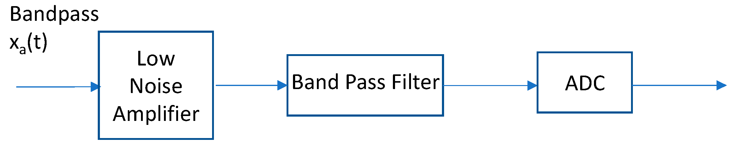
The other approach is to use direct sampling, which can be thought of as a clever and deliberate under-sampling idea [5]. By appropriately selecting the sampling rates, the replicas of the bandpass signals can be down-converted to low frequency regions and recovered there. One key advantage of this direct approach is that mixers and their limitations are all eliminated. However, due to aliasing, background noises in high frequency ranges are all folded into the low-frequency band. As shown in Figure 4, to counteract the noise issue, high-Q bandpass filters are needed to remove out-of-band noises.

2.1.4. Basic Idea of Direct Sampling of Bandpass Signals

Figure 5 shows the definitions of some important parameters in direct bandpass sampling. Here, we briefly summarize the direct sampling idea described in pages 412–415 of [3]. This is for the case where there is no guard band. Referring to Figure 5, in order to avoid aliasing, the sampling frequency should be selected so that the (k − 1)th and the kth shifted replicas of the negative spectral band do not overlap with the positive spectral band. This is achievable if the following conditions are satisfied:

$$2F_H\le k{F}_s$$

(4)

$$\left(k-1\right)F_s\le 2F_L$$

(5)

From (4) and (5), it can be easily seen that

$$\frac{2F_H}{k}\le k{F}_s\le \frac{2F_L}{\left(k-1\right)}$$

(6)

Rewriting (4) and (5) yields

$$\frac{1}{F_s}\le \frac{k}{2F_H}$$

(7)

$$\left(k-1\right)F_s\le 2F_L=2(F_H-B)$$

(8)

Multiplying (7) and (8) gives

$$\left(k-1\right)\le \frac{k\left(2F_H-2B\right)}{2F_H}=k-kB/F_H$$

(9)

Rearranging (8) produces

$$k\le \frac{F_H}{B}$$

(10)

The maximum value for k is the number of bands that we can fit in the range between 0 and $F_H$.

2.2. Problem Statement

When one applies sampling to real applications in communications, radar, and sonar systems, one may face some confusing issues in bandpass sampling. Engineers may have problems in understanding the confusing issues. We will provide details for those issues in Section 2.3.1.

In addition to the above issues, another issue is that there was no explicit formula to compute an integer for determining the allowable sampling frequencies if a specified sampling frequency tolerance is given. Qi et al. [2] proposed a solution for this problem. However, it was not clear how Equation (6) in Qi’s paper was derived. Moreover, the notations in Qi’s paper [2] are quite different from those in [3], making it difficult for engineers to understand.

The purpose of this study is to address the aforementioned issues. Similar to [1,2,3,4], we focus on a single bandpass signal. First, we would like to explain why the issues raised earlier occurred. It is surprising to see that no one has published any papers addressing the above issues since the publication of [1] in 1991. The explanations will help engineers and practitioners avoid some wrong usage of some formulae in bandpass sampling. Second, we address a practical problem in which we are given a specified sampling frequency tolerance and the guard bands in carrier frequency, and we need to determine an appropriate integer for determining the allowable sampling frequencies. We derived a simple and new analytic expression to determine the maximum integer, which plays a critical role in determining the minimum and maximum allowable sampling frequencies. The tolerances in sampling frequency and carrier frequency are important in dealing with oscillator imprecision in analog-to-digital converters (ADC). Explicitly determining the allowable sampling frequencies based on those tolerances will enable fast and easy determination of sampling rates for bandpass applications.

2.3. Root Cause of the Issues and New Results in Bandpass Sampling

2.3.1. Issues

Let us use one example to illustrate the issues. In one example in Chapter 6 of [3], a bandpass signal with a bandwidth of 25 kHz, guard bands of 2.5 kHz, and a carrier frequency of 10,715 kHz needs to be sampled. Following the standard steps in the textbook, one can obtain the minimum and maximum allowable sampling frequencies, which are given as 60.1120 kHz and 60.1124 kHz, respectively. The maximum integer for determining the range of allowable sampling frequencies is 357. It can be seen that the range of allowable sampling frequencies is 0.4 kHz. However, according to Equations (6.4.22) and (6.4.23) in [3], the guard bands can be calculated, which are 35.6 kHz and 35.7 kHz, respectively. These guard band numbers are much larger than the original guard band value of 2.5 kHz in the specification. Engineers and practitioners may be confused and could not understand the root cause of the inconsistencies. These issues or inconsistencies have not been resolved since the publication of [1] in 1991; are unresolved in the 4th edition of [3], which came out in 2007; and still remain unresolved even in the most recent 5th edition that just came out in March 2021 [4].

2.3.2. Root Cause of the Issues

Throughout this paper, we will adopt the notations in Proakis and Manolakis’ book [3], which is one of the most popular textbooks in digital signal processing. Figure 6 shows the various parameters. $F_L$ and $F_H$ denote the lowest and highest frequencies, respectively, of the bandpass signal, which has a bandwidth of B; $∆B_L$ and $∆B_H$ are the guard bands that are used to tolerate some variations in the carrier frequency. Using the above notations, the augmented band locations and bandwidth are given by

$$F_L^{\prime }=F_L-∆B_L,$$

(11)

$$F_H^{\prime }=F_H+∆B_H,$$

(12)

$$B^{\prime }=B+∆B_L+∆B_H.$$

(13)

According to [1,3], the allowable sampling frequency range is given by

$$\frac{2F_H^{\prime }}{k^{\prime }}\le F_s\le \frac{2F_L^{\prime }}{k^{\prime }-1}, \mathrm{where} k^{\prime }=⌊\frac{F_H^{\prime }}{B^{\prime }}⌋.$$

(14)

Here,$k^{\prime }$ in (14) is a critical integer in avoiding aliasing in bandpass sampling, and $⌊\cdot ⌋$ denotes the flooring operation. From (14), the difference between the maximum and minimum allowable frequencies is then given by

$${∆F}_s=\frac{2F_L^{\prime }}{k^{\prime }-1}-\frac{2F_H^{\prime }}{k^{\prime }}$$

(15)

From [1,3], the following relationships were obtained:

$${∆F}_s=\frac{2F_L^{\prime }}{k^{\prime }-1}-\frac{2F_H^{\prime }}{k^{\prime }}={∆F}_{sL}+{∆F}_{sH},$$

(16)

$$∆B_L=\frac{k^{\prime }-1}{2}{∆F}_{sH},$$

(17)

$$∆B_H=\frac{k^{\prime }}{2}{∆F}_{sL}.$$

(18)

We would like to first point out that Equations (16)–(18) are incorrect. The correct expression for $∆F_s$ (Equation (16)) should have been

$$\begin{array}{cc}\hfill {∆F}_s& =\frac{2F_L^{\prime }}{k^{\prime }-1}-\frac{2F_H^{\prime }}{k^{\prime }}\hfill \\ \hfill & =\frac{2F_L}{k^{\prime }-1}-\frac{{2F}_H}{k^{\prime }}-\frac{2∆B_L}{k^{\prime }-1}-\frac{2∆B_H}{k^{\prime }}.\hfill \end{array}$$

(19)

In general, $\frac{2F_L}{k^{\prime }-1}-\frac{{2F}_H}{k^{\prime }}\ne 0$. Hence, it is incorrect to assume ${∆F}_s={∆F}_{sL}+{∆F}_{sH}$ in (16). Because of the above error, (17) and (18) are also incorrect. The above errors were the root cause of the issues raised earlier. In a nutshell, (16)–(18) are incorrect and should not have been used.

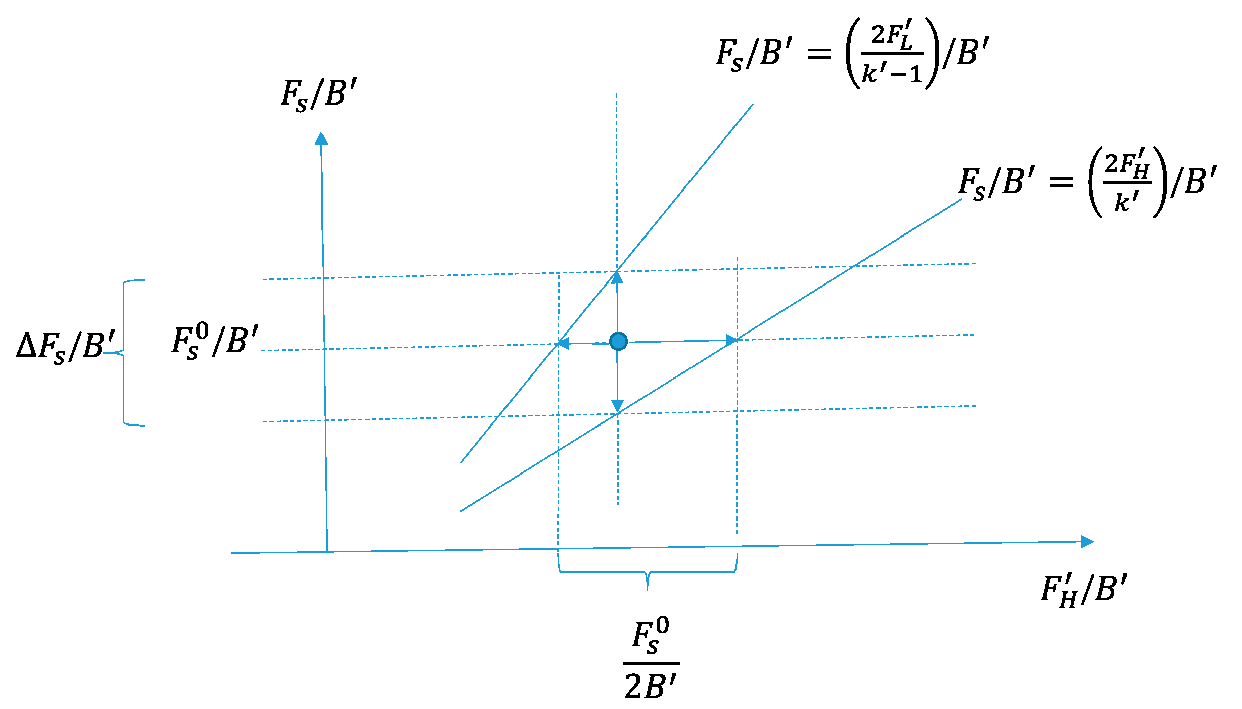
It turns out that the graph in Figure 6.4.4 of [3] is also incorrect. If one chooses the operating sampling frequency to be

$$\begin{array}{cc}\hfill F_s^o& =\frac{\frac{2F_L^{\prime }}{k^{\prime }-1}+\frac{2F_H^{\prime }}{k^{\prime }}}{2}\hfill \\ \hfill & =\frac{F_L^{\prime }}{k^{\prime }-1}+\frac{F_H^{\prime }}{k^{\prime }},\hfill \end{array}$$

(20)

then the correct graphical relationship for the various quantities should be those relations shown in Figure 7. That is, the vertical range in sampling frequency between the two slanted lines at the operating sampling frequency is given by

$$\frac{{∆F}_s}{B^{\prime }}=\left(\frac{2F_L^{\prime }}{k^{\prime }-1}-\frac{2F_H^{\prime }}{k^{\prime }}\right)/B^{\prime }.$$

(21)

The horizontal range between the two slanted lines at the operating sampling frequency is given by

$$\begin{array}{cc}\hfill \frac{∆F}{B^{\prime }}& =\frac{k^{\prime }{F}_s^0}{{2B}^{\prime }}-\frac{{(k}^{\prime }-1)F_s^0}{{2B}^{\prime }}\hfill \\ \hfill & =\frac{F_s^0}{{2B}^{\prime }}.\hfill \end{array}$$

(22)

2.4. New Results

Now, we provide new results for the derivation of $k^{\prime }$ to satisfy a specific sampling frequency tolerance $∆F_s$ and guard bands for tolerating carrier frequency imprecision.

Suppose $∆F_s$ is specified by an engineer to provide tolerance for oscillator errors related to sampling. Moreover, the guard bands are given by those Equations in (11)–(13). Let us denote $∆F_s=2{∆}_s.$ Now, Equation (15) becomes

$${∆F}_s=\frac{2F_L^{\prime }}{k^{\prime }-1}-\frac{2F_H^{\prime }}{k^{\prime }}=2{∆}_s.$$

(23)

Rewriting (13) yields the following quadratic equation;

$$\frac{k^{\prime }{F}_L^{\prime }}{{∆}_s}-\frac{(k^{\prime }-1)F_H^{\prime }}{{∆}_s}=k^{\prime }(k^{\prime }-1).$$

(24)

Solving (24) for $k^{\prime }$, we can easily obtain the solution for a positive $k^{\prime }$, which is given by

$$k^{\prime }=⌊\frac{-b+\sqrt{b^2-4c}}{2}⌋$$

(25)

where

$$\begin{array}{c}b=-1-\frac{F_L^{\prime }}{{∆}_s}+\frac{F_H^{\prime }}{{∆}_s},\hfill \\ c=-\frac{F_H^{\prime }}{{∆}_s}.\hfill \end{array}$$

The other solution of (24) gives a negative number for $k^{\prime }$ and hence is discarded. Using the $k^{\prime }$ from (25), we can then use Equation (24) to determine the range of allowable sampling frequencies that satisfy all the specifications related to the guard bands ($∆B_L and ∆B_H$) and sampling frequency tolerance (${∆F}_s)$.

It is emphasized that the equation in (15) is new and different from that of [2].

3. Examples

In this section, we will include two examples to illustrate the raised issues and the new results.

3.1. Example 1

Let us assume B = 200 kHz, $F_L=103.4 \mathrm{MHz}$, $F_H=103.6 \mathrm{M}\mathrm{H}\mathrm{z}$, $∆B_L$ = $∆B_H$ = 20 kHz, and ${∆}_s=10 \mathrm{k}\mathrm{H}\mathrm{z}$. From (25), we obtain $k^{\prime }=90$. From (14), we then obtain the following range of sampling frequencies:

$${2302.6667 \mathrm{k}\mathrm{H}\mathrm{z}\le F}_s\le 2323.1461 \mathrm{k}\mathrm{H}\mathrm{z}.$$

(26)

From (26), the allowable sampling frequency range is ${∆F}_s=20.4794 \mathrm{k}\mathrm{H}\mathrm{z}.$ Using (20), we can select the operating sampling frequency to be

$$F_s^o=2312.9064 \mathrm{k}\mathrm{H}\mathrm{z}.$$

Using the given parameters mentioned earlier, we can also calculate $\frac{2F_L}{k^{\prime }-1}-\frac{{2F}_H}{k^{\prime }}$, which is nonzero and equals 21.373 kHz. Comparing (16) and (19), one can easily deduce that (16) is incorrect. To demonstrate that the formulae (17) and (18) are also incorrect, we first calculate ${∆F}_{sH}$ and ${∆F}_{sL}$ using (17) and (18), which gives

$${∆F}_{sH}=449.4382 \mathrm{H}\mathrm{z}$$

$${∆F}_{sL}=444.44 \mathrm{H}\mathrm{z}.$$

In this example, one can easily see that ${∆F}_s$ is actually 20.4794 kHz, not (449.4382 + 444.44 Hz). Hence, ${∆F}_s\ne {∆F}_{sH}+{∆F}_{sL}$.

The horizontal frequency range in Figure 7 is calculated as $\frac{F_s^0}{{2B}^{\prime }}=4.8186$. On the other hand, if we use the formulae in the textbook for the range of horizontal frequency, we obtain $\frac{∆B_L}{B^{\prime }}+\frac{∆B_H}{B^{\prime }}=\frac{40 \mathrm{k}\mathrm{H}\mathrm{z}}{240 \mathrm{k}\mathrm{H}\mathrm{z}}=0.1667$, which is clearly incorrect.

From the above calculations, we observe that the allowable operating sampling frequency without causing aliasing is nearly 10 times the bandpass signal bandwidth. This example clearly shows that, for practical applications where there may be oscillator imprecision, bandpass sampling will require a much higher sampling frequency (at least in this example) than that of using the mixer and in-phase and quadrature phase approach, in which only two times the bandwidth of the ELP signal is required. It should be noted that the selected sampling frequency depends on the sampling tolerance. For small sampling tolerance (precise and accurate sampler), the required sampling frequency will be smaller.

3.2. Example 2

Here, we would like to use the same example in [2] for illustration. In terms of the notations of [2], the carrier frequency ($F_c$) is 140 MHz, the bandwidth (B) of the ELP signal is 12.5 MHz, the tolerance for carrier frequency (${∆}_c$) is 900 kHz, and the tolerance for sampling frequency (${∆}_s$) is 14 kHz. To be compatible with the notations in this paper, we first convert the above numbers into the following:

$$F_L=F_c-\frac{B}{2}=133.75 \mathrm{M}\mathrm{H}\mathrm{z},$$

$$F_H=F_c+\frac{B}{2}=146.25 \mathrm{M}\mathrm{H}\mathrm{z},$$

$$∆B_L=∆B_H=\frac{{∆}_c}{2}=450 \mathrm{k}\mathrm{H}\mathrm{z},$$

$${∆}_s=14 \mathrm{k}\mathrm{H}\mathrm{z},$$

$$F_L^{\prime }=F_L-∆B_L=133.3 \mathrm{M}\mathrm{H}\mathrm{z},$$

$$F_H^{\prime }=F_H+∆B_H=146.7 \mathrm{M}\mathrm{H}\mathrm{z},$$

$$B^{\prime }=B+∆B_L+∆B_H=13.4 \mathrm{M}\mathrm{H}\mathrm{z}.$$

Using (25), we obtain $k^{\prime }=10$. Consequently, the range of allowable sampling frequencies is given by

$${29.34 \mathrm{M}\mathrm{H}\mathrm{z}\le F}_s\le 29.62 \mathrm{M}\mathrm{H}\mathrm{z}.$$

(27)

If we choose the operating sampling frequency to be the average of the above frequencies in (27), we obtain $F_s^o=29.48 \mathrm{M}\mathrm{H}\mathrm{z}$, which is very close to the results in [2] (29.43 MHz). The difference between the maximum and minimum sampling frequency is 29.62 − 29.34 = 0.28 MHz, which is much larger than the originally specified value of ${2∆}_s=$ 2 × 14 kHz, meaning that we satisfy the design specification by a big margin. The main reason for this excessive margin is attributed to the floor operation in obtaining $k^{\prime }$. The exact root obtained by solving the quadratic equation is 10.836. The flooring operation gives a larger range than necessary. Actually, the chosen $k^{\prime }$ can tolerate close to 140 kHz of the oscillator error.

In this example, we can also see that (17) and (18) are incorrect because using (17) and (18) yields

$$\begin{gathered} { ∆F}_{sH}=100 \mathrm{k}\mathrm{H}\mathrm{z} \\ {∆F}_{sL}=90 \mathrm{k}\mathrm{H}\mathrm{z}. \end{gathered}$$

We ${∆F}_s=0.28 \mathrm{M}\mathrm{H}\mathrm{z}$ obtained from (27) does not equal ${∆F}_{sH}+{∆F}_{sL}=190 \mathrm{k}\mathrm{H}\mathrm{z}$, indicating that those noted in Equations (16)–(18) are incorrect.

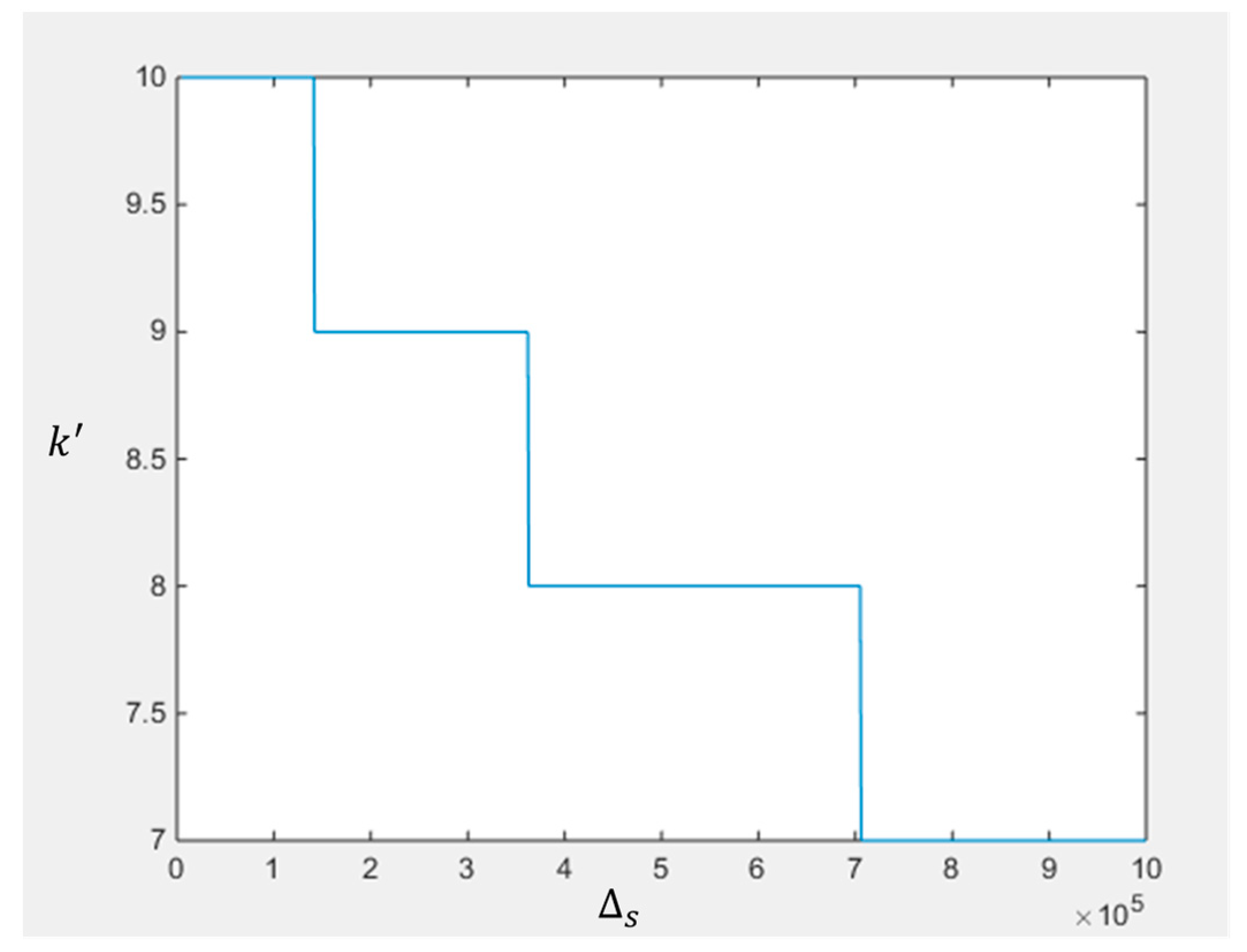
It will be interesting to plot the $k^{\prime }$ values for different tolerance of ${∆}_s$ in this example. Because of the floor operation, it can be seen from Figure 8 that a single $k^{\prime }$ can be used to tolerate a range of ${∆}_s.$ Codes for generating Figure 8 are included in Appendix A.

4. Conclusions and Future Directions

In this study, we first pointed out some errors related to bandpass sampling in [1,3,4]. It is emphasized that these errors went un-noticed since 1991. The root cause for the errors was determined and explained. A correct graphical illustration was then presented. Second, given a sampling frequency tolerance (${∆}_s$) and some guard bands for the bandpass signal, we presented a simple and new analytic formula for determining an integer that is critical in determining the allowed range of sampling frequencies. This is an important contribution to bandpass sampling, as engineers and practitioners can correctly determine the allowable sampling frequencies based on some specified guard bands and sampling frequency tolerance. Examples were provided to illustrate the proposed solutions as well as those raised errors in the literature.

There are two future research directions. First, it will be an important contribution to explicitly incorporate sampling rate uncertainties into those iterative methods in [5,6,7,8,9,10,11]. Second, it will be also important to extend the proposed method in this paper to multiple bandpass signals.

References

- Vaughan, R.G.; Scott, N.L.; White, D.R. The theory of bandpass sampling. IEEE Trans. Signal Process. 1991, 39, 1973–1984. [Google Scholar] [CrossRef]
- Qi, R.; Coakley, F.P.; Evans, B.G. Practical consideration for bandpass sampling. Electron. Lett. 1996, 32, 1861–1862. [Google Scholar] [CrossRef]
- Proakis, J.G.; Manolakis, D.G. Digital Signal Processing: Principles, Algorithms and Applications, 4th ed.; Pearson Prentice Hall: London, UK, 2007. [Google Scholar]
- Proakis, J.G.; Manolakis, D.G. Digital Signal Processing: Principles, Algorithms and Applications, 5th ed.; Pearson Prentice Hall: London, UK, 2021. [Google Scholar]
- Akos, D.M.; Stockmaster, M.; Tsui, B.Y.; Casschera, J. Direct bandpass sampling of multiple distinct RF signals. IEEE Trans. Commun. 1999, 47, 983–987. [Google Scholar] [CrossRef]
- Wong, N.; Ng, T.S. An efficient algorithm for downconverting multiple bandpass signals using bandpass sampling. Proc. IEEE Int. Conf. Commun. Helsinki 2001, 13, 910–914. [Google Scholar]
- Choe, M.; Kim, K. Bandpass sampling algorithm with normal and inverse placements for multiple RF signals. IEICE Trans. Commun. 2005, E88, 754–757. [Google Scholar] [CrossRef]
- Tseng, C.-H.; Chou, S.-C. Direct Downconversion of Multiband RF Signals Using Bandpass Sampling. IEEE Trans. Wirel. Commun. 2006, 5, 72–76. [Google Scholar] [CrossRef]
- Bae, J.; Park, J. An efficient algorithm for bandpass sampling of multiple RF signals. IEEE Signal Process. Lett. 2006, 13, 193–196. [Google Scholar] [CrossRef]
- Bose, S.; Khaitan, V.; Chaturvedi, A. A Low-Cost Algorithm to Find the Minimum Sampling Frequency for Multiple Bandpass Signals. IEEE Signal Process. Lett. 2008, 15, 877–880. [Google Scholar] [CrossRef]
- Liu, J.-C. Bandpass Sampling of Multiple Single Sideband RF Signals. In Proceedings of the ISCCSP 2008, St. Julians, Malta, 12–14 March 2008. [Google Scholar]
- Thombre, S.; Nurmi, J. Bandpass-Sampling Based GNSS Sampled Data Generator—A Design Perspective. In Proceedings of the 2012 International Conference on Localization and GNSS, Starnberg, Germany, 25–27 June 2012; pp. 1–6. [Google Scholar] [CrossRef]
- Lesnikov, V.; Naumovich, T.; Chastikov, A. Dealiasing Technique for Processing of Sub-Nyquist Sampled Bandpass Analytic Signals. In Proceedings of the 2021 International Siberian Conference on Control and Communications (SIBCON), Kazan, Russia, 13–15 May 2021; pp. 1–6. [Google Scholar] [CrossRef]
- Zhang, X.Y.; Xu, X.J.; Zou, Y.X. Sampling jitter mitigation with a cascade multiplier for direct RF bandpass sampling receiver. In Proceedings of the17th International Conference on Advanced Communication Technology (ICACT), PyeongChang, Republic of Korea, 1–3 July 2015; pp. 413–418. [Google Scholar] [CrossRef]
- Lesnikov, V.; Naumovich, T.; Chastikov, A. Aliasing’s Study on Bandpass Sampling. In Proceedings of the 2022 Systems of Signal Synchronization, Generating and Processing in Telecommunications (SYNCHROINFO), Arkhangelsk, Russia, 29 June–1 July 2022; pp. 1–6. [Google Scholar] [CrossRef]
- Lesnikov, V.; Naumovich, T.; Chastikov, A.; Dubovcev, D. Sub-Nyquist Bandpass Sampling. In Proceedings of the 2023 25th International Conference on Digital Signal Processing and Its Applications (DSPA), Moscow, Russia, 29–31 March 2023; pp. 1–6. [Google Scholar] [CrossRef]
- Wahab, M.; Levy, B.C. Quadrature Filter Approximation for Reconstructing the Complex Envelope of a Bandpass Signal Sampled Directly with a Two-Channel TIADC. IEEE Trans. Circuits Syst. II Express Briefs 2022, 69, 3017–3021. [Google Scholar] [CrossRef]
- Liu, Z.; Feng, X.; Chen, S. Time Encoding Sampling of Bandpass Signals. In Proceedings of the 2023 31st European Signal Processing Conference (EUSIPCO), Helsinki, Finland, 4–8 September 2023; pp. 1898–1902. [Google Scholar] [CrossRef]
Figure 1.
Illustration of sampling and aliasing phenomena.
Figure 2.
Bandpass signals.
Figure 3.
Bandpass sampling using mixers and in-phase and quadrature phase signals.
Figure 4.
Direct bandpass sampling without mixers.
Figure 5.
Definition of some parameters in direct bandpass sampling.
Figure 6.
Bandpass signal with guard bands.
Figure 7.
Graphical illustration of the various relationships between the operating sampling frequency and other variables.
Figure 8.
Plot of sampling tolerance vs. .
Disclaimer/Publisher’s Note: The statements, opinions and data contained in all publications are solely those of the individual author(s) and contributor(s) and not of MDPI and/or the editor(s). MDPI and/or the editor(s) disclaim responsibility for any injury to people or property resulting from any ideas, methods, instructions or products referred to in the content. |
© 2024 by the author. Licensee MDPI, Basel, Switzerland. This article is an open access article distributed under the terms and conditions of the Creative Commons Attribution (CC BY) license (https://creativecommons.org/licenses/by/4.0/).
Share and Cite
MDPI and ACS Style
Kwan, C. Issues and New Results on Bandpass Sampling. Electronics 2024, 13, 280. https://doi.org/10.3390/electronics13020280
AMA Style
Kwan C. Issues and New Results on Bandpass Sampling. Electronics. 2024; 13(2):280. https://doi.org/10.3390/electronics13020280
Chicago/Turabian StyleKwan, Chiman. 2024. "Issues and New Results on Bandpass Sampling" Electronics 13, no. 2: 280. https://doi.org/10.3390/electronics13020280
Note that from the first issue of 2016, this journal uses article numbers instead of page numbers. See further details here.