Evaluating Explainable Artificial Intelligence Methods Based on Feature Elimination: A Functionality-Grounded Approach

Abstract

Although predictions based on machine learning are reaching unprecedented levels of accuracy, understanding the underlying mechanisms of a machine learning model is far from trivial. Therefore, explaining machine learning outcomes is gaining more interest with an increasing need to understand, trust, justify, and improve both the predictions and the prediction process. This, in turn, necessitates providing mechanisms to evaluate explainability methods as well as to measure their ability to fulfill their designated tasks. In this paper, we introduce a technique to extract the most important features from a data perspective. We propose metrics to quantify the ability of an explainability method to convey and communicate the underlying concepts available in the data. Furthermore, we evaluate the ability of an eXplainable Artificial Intelligence (XAI) method to reason about the reliance of a Machine Learning (ML) model on the extracted features. Through experiments, we further, prove that our approach enables differentiating explainability methods independent of the underlying experimental settings. The proposed metrics can be used to functionally evaluate the extent to which an explainability method is able to extract the patterns discovered by a machine learning model. Our approach provides a means to quantitatively differentiate global explainability methods in order to deepen user trust not only in the predictions generated but also in their explanations.

1. Introduction

As solutions based on Machine Learning (ML) are used in nearly every business domain, the efficiency of decision-making and related tasks increases. However, the efficiency of ML-based solutions is proportionally related to their complexity. As the accuracy and efficiency of such solutions increase, their complexity increases while reducing human interpretability. To address the need of making ML-based solutions understandable and interpretable to users, ML researchers have suggested a plethora of methods under the umbrella of eXplainable AI (XAI) [1,2,3,4,5].

1.1. Problem Statement

XAI methods are linked with varying goals, scopes, analysis techniques, user groups, and output formats. However, the vast availability of divergent XAI methods raises the challenge of the need to systematically evaluate and compare them. Evaluating XAI methods still constitutes a gap in XAI research gap. In particular, a comprehensive evaluation method, which is neither specific to a particular data type (e.g, tabular, text, or images) nor to an XAI method, is still lacking. Contemporary XAI evaluation methods follow different goals that include: (1) the evaluation of the understandability and clarity of XAI outcomes to humans, (2) the ability of humans to perform further tasks depending on their understanding of the XAI outcomes, and (3) the correctness and precision of an explanation generated by an XAI method. Furthermore, XAI methods are evaluated either quantitatively or qualitatively with respect to the first two evaluation goals. Most proposals that address the third evaluation goal provide quantitative approaches to measure a certain characteristic of the respective XAI method or its outcomes. For example, the stability of explanations is measured by [6] and fidelity by [7,8], whereas the robustness of XAI methods is evaluated by [9].

1.2. Contributions

This article proposes a novel approach to evaluate the explanations generated by XAI methods. This approach deals with the issue of how consistent an explanation is, in terms of its constituting features, with a feature set that influences the dependent variable. Ref. [10] refers to consistency as the similarity of the explanations generated for similar predictions made by two different ML models that are trained on the same task. This paper uses the term consistency to denote the similarity between the ground truth and the explanations generated using different XAI methods that explain the predictions of the same ML model. In our context, similarity expresses the amount of shared knowledge. By ground truth, in turn, we mean extracted knowledge about the features that are expected to drive a prediction. These features drive the prediction process by having a strong relation to the dependent variable and influencing its value. In a nutshell, the proposed approach comprises the following basic stages:

• Analysis of the dataset to identify a set of features, that are considered indispensable for the prediction process (ground truth extraction).
• Extracting the features that are actually used by the ML model, based on the explanations proposed by different XAI methods.
• Computing the consistency value for the feature set suggested by each XAI method.
• Comparing different XAI methods based on their ratios according to the model selection metrics we propose.

Our main contributions can be summarised as follows:

• We develop an approach to extract a representation of the most influencing features in a given dataset. We denote these features as indispensable ones.
• We introduce a consistency value that measures knowledge shared between the feature set obtained with XAI methods and the computed indispensable features.
• We customize two well-known model selection metrics to incorporate three dimensions of the problem space; namely, the feature set highlighted by an XAI method, its relevant consistency value, and the sample size. This sample is the one used in training the ML model and for which explanations are generated by the XAI method under analysis.

The remainder of this paper is structured as follows. In Section 2, we provide backgrounds on approaches and techniques required for understanding this paper. Section 3 deals with the addressed research questions. The approach and the main contributions of this work are presented in Section 4. In Section 5, we define the settings of the experiments we conducted to evaluate the approach. Experimental results are presented in Section 6. Section 7 discusses related work followed by a summary and outlook in Section 8.

2. Backgrounds

The aim of the proposed approach is to quantitatively evaluate explainability outcomes as an integrated part of an ML-based prediction process. In the following, we highlight the most relevant concepts needed to understand our approach.

2.1. Explainable Artificial Intelligence

ML-based models codify the past, whereas they are unable to control the future. Moreover, biases do not only occur due to the malfunctioning pattern learning of the ML model but might be also caused by unobserved biases in the dataset that is used for the learning process. For example, consider a dataset whose entries mostly refer to male employees and are collected only for a segment of male employees with more years of experience. Note that such an imbalance in the collected data might lead to a conclusion that males are gaining more income than their female colleagues even with the same years of experience. An ML model trained on such a dataset might mistakenly infer that the gender feature is highly correlated with high-income rates rather than the expertise level or the organizational section the employees belong to. Therefore, identifying biases or problems in the past reasoning process might enable us to prevent them in the future or at least to be aware of the potential to encounter the same bias.

Ref. [11] discusses numerous cases of black box ML models generating an unjustified prediction based on biased data or unreasonably learned patterns from a human perspective. Such predictions were used to guide the human decision-making process, leading to wrong decisions in many cases [11]. Gaining insights into the learning and reasoning process of an ML model, therefore, becomes crucial, as ML models are increasingly integrated into our daily lives and affect critical decisions made by governmental, medical, and other entities. In response to this need, eXplainable Artificial Intelligence (XAI) emerged as a subfield of AI and ML.

Since the ML community started to emphasize the importance of understanding the behavior of ML models, there has been no agreed-upon definition of explainability. Explainability represents the potential to provide an illustration of the model reasoning process in terms of the features contributing to its outcome [12]. Over the last years, several authors (e.g., Carvalho et al. [10], Guidotti et al. [11], Vilone and Longo [12], Jesus et al. [13] Barredo Arrieta et al. [14]) have tried to determine requirements that, if met, will allow characterizing an explanation and evaluating an XAI method. Most research works agreed upon certain desiderata of an XAI method:

• Robustness, meaning that an explanation can withstand small perturbations of the input that do not change the output prediction [12]. Consequently, robustness expresses a low sensitivity of the XAI method to changes in inputs.
• Fidelity, meaning that the XAI method should preserve the internal concepts and original behavior of the black box ML model whenever there is a need to mimic that model.
• Causality, meaning that the XAI method should maintain causal relationships between inputs and outputs. Note that an ML model is perceived as being more human-like whenever it provides such causal explanations. Therefore, causality is fundamental to achieving a human understanding of the ML model.
• Trust, meaning that the outcomes of an XAI method enable gaining confidence that the ML model acts as intended.
• Fairness, meaning that an explanation has to enable humans to ensure unbiased decisions of the employed ML models.

There are other characteristics such as, for example transferability, informativeness, transparency, privacy, and accessibility. Moreover, characterizing an explanation or XAI method might be case-dependent and shaped by domain requirements. Finally, XAI methods may be grouped into different categories reflecting different perspectives of explainability. In detail, these categories are:

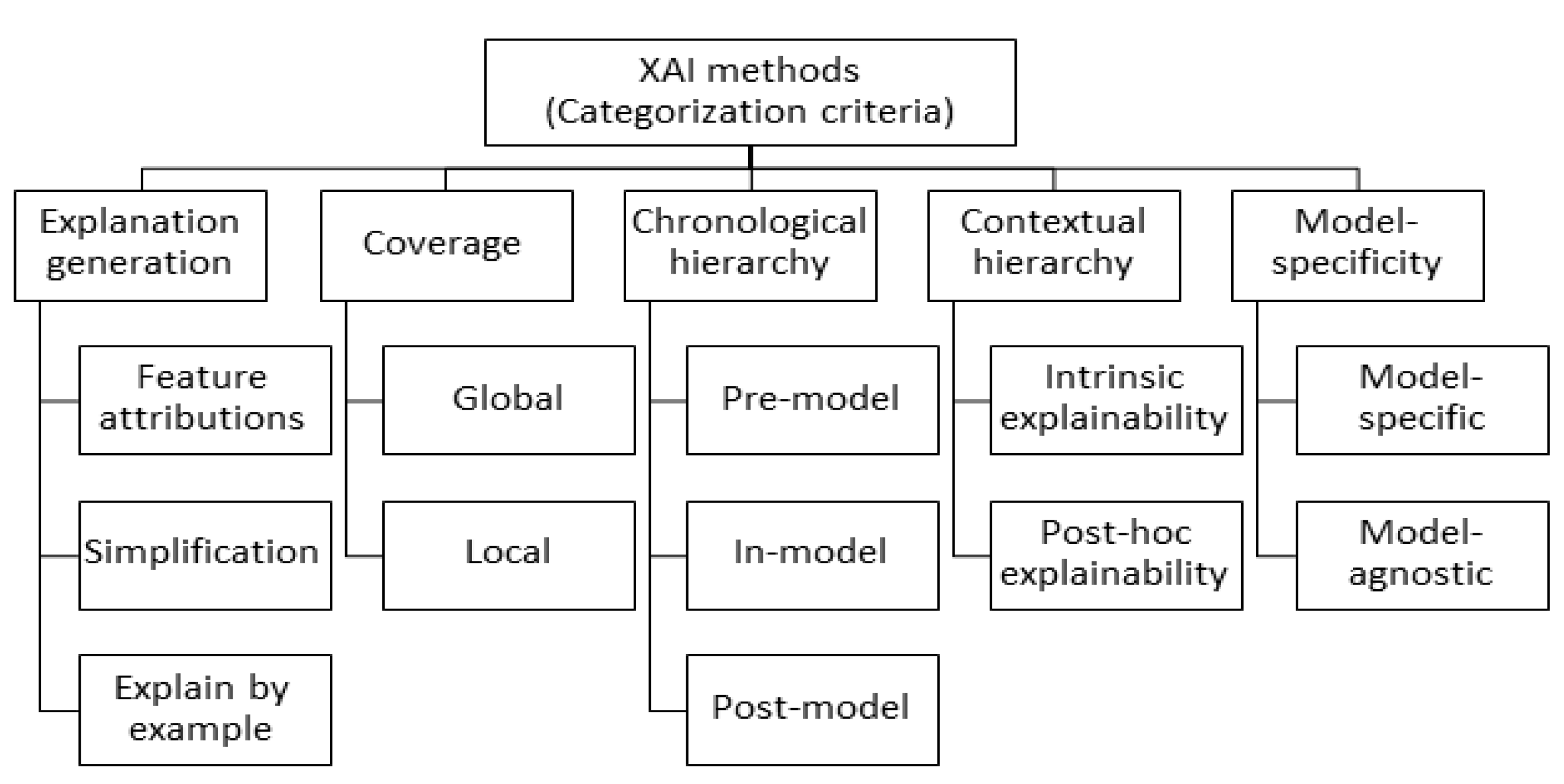
• Explanation generation. The explanation generation approach represents a crucial categorization dimension of XAI methods. The selection of a specific explanation form depends on the level of complexity of the explanation to be conveyed as well as the expertise level of the end user. Refs. [14,15] refer to certain explanation forms. First, feature attributions represents a commonly used explanation form where the relevance or the explanatory power of the features is computed with respect to predictions generated by the original model. Second, Simplification uses an interpretable simpler model to mimic and explain the behavior of the original model. Finally, explain-by-example constitutes another form of explanation where a prediction corresponding to a sample is explained by finding a similar sample with a counterpart prediction or a different sample with a similar prediction.
• Coverage. XAI methods are either global or local. Global explainability methods generate explanations that summarize patterns learned by an ML model over a large number of samples. These methods tend to understand the distribution of the prediction output space in terms of the input features [10]. In turn, local explainability methods study the interactions between patterns to better understand how a specific input led to a certain output in a given sample [16]. Consequently, local explainability methods generate explanations for a single sample or a group of similar samples.
• Chronological hierarchy. [10] groups XAI methods with respect to the point in time an XAI method is applied with respect to the modeling step. First, Pre-Model Explainability means that the XAI method is applied to the dataset itself regardless of the modeling step. Methods falling into this category tend to adopt exploratory and presentation perspectives of the input data. Second, In-Model Explainability means producing explanations as part of the model training process. Finally, Post-Model Explainability means producing explanations for predictions of an ML model as a post-momentum step after training the model on historical data.
• Contextual hierarchy. Another criterion is concerned with the ability of an ML model to provide explanations of the predictions by itself or a separate XAI method is applied. In this context, intrinsic explainability means having models that are interpretable by nature, i.e., models that show a high degree of transparency in terms of being simulatable, algorithmically transparent, and decomposable [14]. Linear models and simple decision trees provide common examples of ML models with inherent explainability. Post-hoc explainability targets complex models, which are not interpretable by design. XAI methods in this category are applied to a trained model to reverse engineer the reasoning process of the analyzed ML model.
• Model specificity. The influence of the executed ML model on the choice of an XAI method. Model-specific explanation methods are limited to specific models, as the XAI methods have been tailored towards specific model internals [10]. For example, Layer-wise Relevance Propagation (LRP) [1] and Saliency Maps [5] are specific XAI methods used in the context of models based on neural networks. In turn, model-agnostic methods are applicable to any ML model independent from its internals [16]. Model-agnostic methods incorporate predictors which untied to a particular type of black box, explanation, or data type [11]. LIME [2] and SHAP [3] are examples of the latter subcategory.

Figure 1 summarizes the categorization criteria for XAI methods. Note that some of these criteria define the relation between the XAI method on one hand and the explained ML model on the other. Other criteria, in turn, define how an XAI method processes its inputs or represents its outputs. The proposed approach is meant to provide an evaluation approach of model-agnostic, global, and post-hoc XAI methods. We advocate evaluating model-agnostic, post-hoc XAI methods in order to offer broad applicability to our proposal. Being limited to a certain category of XAI methods restricts the number of XAI methods our approach is applicable to, for example as in the case of evaluating XAI methods that explain the predictions of deep learning models. The proposed approach evaluates global XAI methods since the core idea of our approach is to measure the consistency with ground truth extracted from the entire dataset. As a result, we need to study the group of XAI methods that examine the reasoning process of an ML model over the entire dataset rather than on single predictions.

2.2. Evaluation of Explainability Methods

The nature and definitions of the XAI methods characteristics presented in Section 2.1 imply that not all of them can be easily quantified. Further, note that an explanation is a subjective matter that is affected by various factors, including user experience and domain knowledge, explanation purpose, techniques to generate the explanation, and explanation scope [15]. Various approaches are proposed to evaluate the quality of an explanation. Ref. [17] assigns these evaluation approaches to three categories:

• Application-grounded evaluations imply the use of the ML-based solution in a real-life application, generate explanations for the users of this application, and evaluate the quality of an explanation in the context of real-life tasks.
• Human-grounded evaluations aim to evaluate general criteria with respect to explanation quality. Corresponding evaluations create simplified tasks that resemble the real-life application subject of the ML system. Humans involved in these experiments are less experienced than the ones involved in application-grounded evaluations.
• Functionally-grounded evaluations. In this category, no humans are involved. Instead, some formal definitions of interpretability are considered to form a proxy of explanation quality. Corresponding evaluations are objective (unlike the former categories) and depend on quantitative metrics [15]. These evaluations are suitable if the cost and time budgets for human-based experiments are limited or the explainability technique to be evaluated is not mature enough and still under iterative development.

Developing means to evaluate explainability techniques allows us to determine the extent to which a particular technique can fulfill explainability goals. Furthermore, evaluating explanation techniques enables us to assess the suitability of specific techniques in a certain context, e.g., if input data is changing over time or computational resources are limited. Our proposed approach is meant to be a functionally-grounded explanation evaluation approach.

2.3. Feature Selection

Generating predictions for highly dimensional datasets mandates finding a compromise between prediction accuracy and computation efficiency. Moreover, for a dataset being both highly dimensional and having only a small number of samples, the ML process itself becomes more complicated. In general, it turns out to be difficult for any ML model to distinguish relevant data from noise as the search space gets sparsely populated with a lower number of samples [18].

Feature set reduction becomes crucial in this context. The ultimate goal of feature reduction is to obtain a minimal feature subset that maximizes the efficiency of the analysis. With analysis, we mean whether the resulting feature subset shall be used in classification, regression, or clustering analysis tasks. With efficiency, we mean the efficient use of computational resources in the analysis of the selected feature set in terms of computation time, storage, and processing. Feature set reduction may be achieved through feature set extraction or feature selection (FS) [19].

In this context, we are interested in feature selection as its related methods provide a minimal feature set without the need for transforming values in this feature set. Consequently, further processing (e.g., explanations of predictions) is based on the original values of the selected features; but neither on transformed nor concluded values. The selected features are supposed to describe the observed phenomena with fewer storage and processing demands. Furthermore, these features contain the maximum discrimination information about the dependent variable.

According to [18], feature selection is the process of detecting the relevant features and discarding the irrelevant ones. Feature relevance is the extent to which a feature contains useful information useful to make predictions and the way this information might be used to decide against or in favor of a certain prediction [20]. Ref. [19] distinguishes between relevance and repetition as two basic characteristics for selecting a feature set. Finally, the selected feature set should maximize relevance and minimize repetition with respect to the analysis goal [19].

Feature selection methods employ four basic steps [19]. First, a method begins with searching for a suitable feature subset from the entire feature set. Second, the selected subset is evaluated according to specific criteria. Third, a stopping criterion is employed to terminate the search for additional features to be included in the selected feature subset. Finally, the selected subset is validated by using it in the analysis task for which the feature set is reduced. Feature selection methods can be categorized into three families:

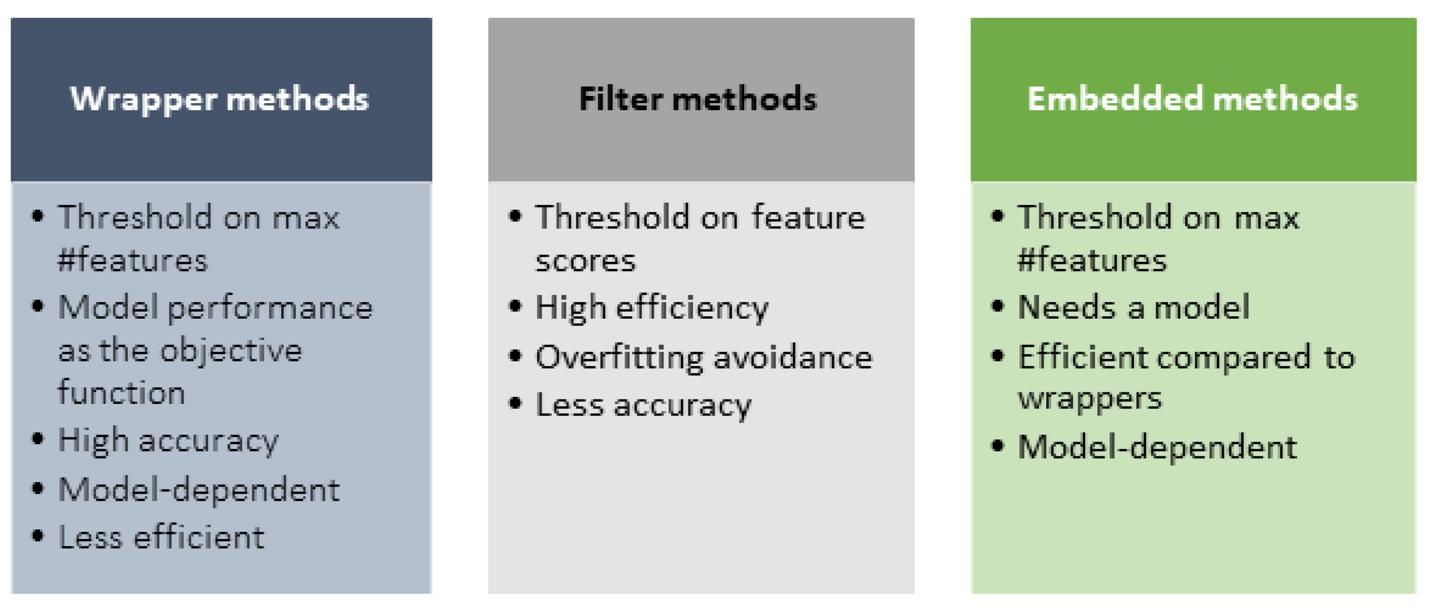
• Wrapper methods. A prediction model is wrapped into the optimal feature subset search step. The selected feature subset is the one that maximizes the performance of the used prediction model [20]. These methods apply a greedy approach for selecting a feature as they consider all possible features with respect to an evaluation criterion [21]. There is one category of methods in this family for which the method begins with an empty feature subset and proceeds forward by adding more features one by one until meeting a stopping criterion. There is another category in which the methods start with the entire feature set and remove features one by one till the predetermined stopping criterion is met. At each step, a new model is trained. Due to the slow computations associated with these methods, wrapper methods have proven to be less efficient despite being more accurate [18].
• Filter methods [20]. Each method belonging to this category utilizes a ranking criterion for ordering the feature set. A selection threshold is used to determine the relevance of a certain feature to the dependent variable. Dependencies between features are not essential to determine whether a particular feature is relevant, i.e., these methods do not take feature interactions into account. However, to be relevant, a feature has to be strongly related to the dependent variable [20]. Note that methods of this category do not rely on any underlying ML model [21].
• Embedded methods. The selection step is an inherent part of the training process when the model assigns some weights or ranks to the features. Common embedded methods include decision tree methods (e.g., CART) and linear models (e.g., linear regression).

Figure 2 summarises the basic properties of each category of feature selection methods. Common to the wrapper and embedded methods is the employment of an ML model at a certain point independent of whether the selection step is part of the model or the model is used as part of the selection process. Filter methods, in turn, study the inherent characteristics of a dataset and the relations between its features to find an optimal or sub-optimal feature subset. Selected features are expected to be more relevant to the analysis goal, and additionally hold minimal information in common with other features (i.e., less redundant).

3. Research Questions

Our goal is to propose an approach that enables differentiating between XAI methods in a functionally-grounded way. We need to distinguish XAI methods with respect to their ability to reflect underlying data facts, under the same prediction settings. For this purpose, we define two research questions.

• RQ1: Given an ML model, how can we identify a feature subset that has the potential to influence the prediction process of this model?

When generating predictions, an ML model depends on the relations and interactions between features on one hand and the dependent variable on the other. If there is a means to obtain features with the highest influence on the dependent variable, this will be a step toward understanding which features are supposed to affect the prediction process. We denote these features as the indispensable features. In this paper, it is out of scope to study whether an ML model has already been used them. However, it should be possible to identify the features that are supposed to guide the prediction process and, hence, may be present in an explanation in an advanced stage. Each ML model has its own sensitivities when concluding relations between features. As a result, we need to introduce a technique that is model-independent. Simultaneously, the proposed technique has to provide insights into the relations between the features and the dependent variable from a data perspective and based on data analysis.

• RQ2: How to use the discovered ground truth as a basis to differentiate global XAI methods?

The proposed approach examines the consistency of an XAI method with respect to the ground truth. To achieve this goal, we address the global XAI methods that investigate how an ML model selects features with a high predictability power for the prediction process. If the indispensable features have the potential to influence the prediction process, they have to be captured by an XAI method and be present in an explanation. To answer RQ2 we need to measure the proximity of the feature set in an explanation to the indispensable features. Furthermore, we need to introduce proper metrics to differentiate XAI methods regarding their proximity in terms of the number of features and, if possible, the magnitude of their importance as indicated by an XAI method.

4. Proposed Approach

We present our approach along four stages that complement each other but differ with respect to the goals they address. Stage 1 is concerned with the data perspective in the context of a prediction generation and explanation pipeline. Stage 2 deals with the analysis of explainability step outcomes. Stage 3 computes a ratio that represents a starting point to qualify the shared knowledge between explanations of an XAI method and the facts extracted in Stage 1. Stage 4 is concerned with comparing multiple XAI methods using facts learned about the data. Figure 3 summarizes the proposed approach and shows the possible outputs of each stage. Note that we add stage (*) in Figure 3, which is “ML model training’’, to keep the approach conformance to the logical sequence of a prediction generation and explanation pipeline. However, we do not propose any additional procedures to the steps held in the respective (*) stage.

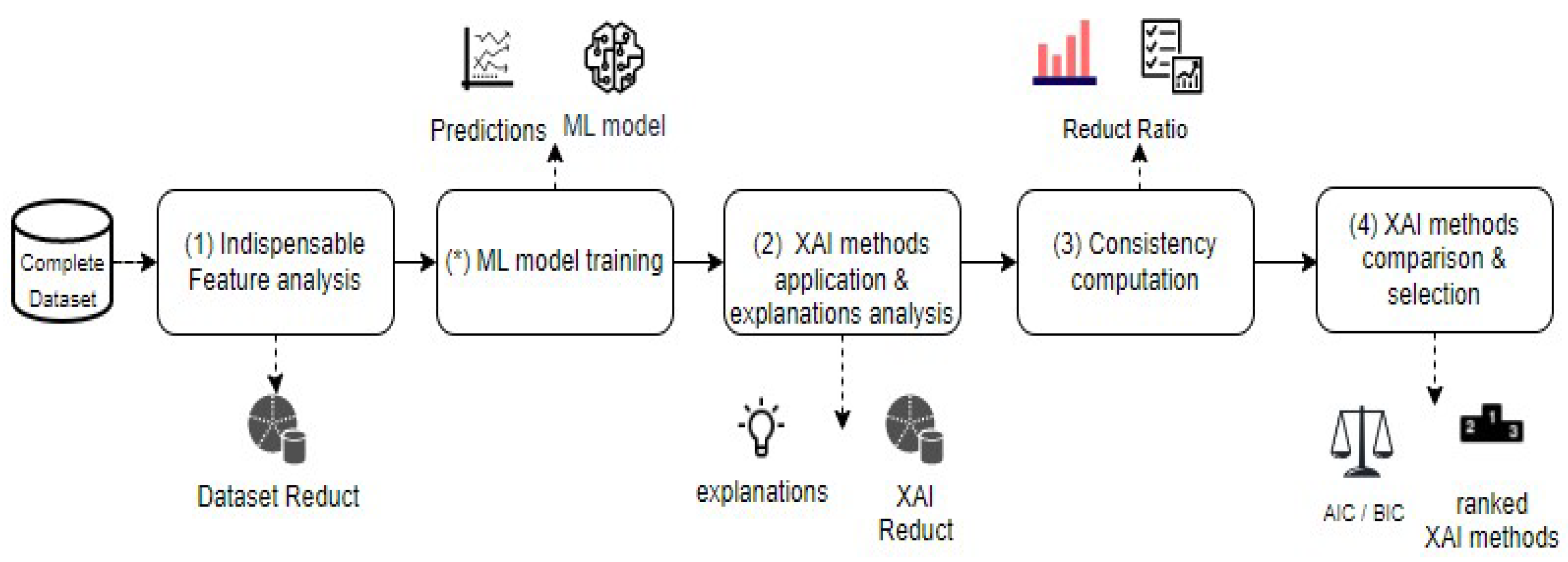
4.1. Stage 1: Indispensable Features Analysis

The goal of Stage 1 is to obtain a ground truth about the data at hand. This ground truth is essential to study the most influencing factors when generating a prediction. Therefore, the steps followed in this Stage are model-independent and aim to extract knowledge from a data perspective. The choice of a specific ML algorithm in the model training phase does not influence the analysis executed in this stage. We pursue a basic understanding of the data apart from the conclusions made by an ML model or obtained after applying an XAI method. Algorithm 1 summarizes the steps executed in Stage 1.

We need to study the relationship between the features and the dependent variable (i.e., the label) from a data perspective. Furthermore, we need to extract a subset of features that are sufficient to drive the prediction process. To analyze the relationship between the features and the dependent variable, we apply a set of feature selection methods that vary in their underlying mechanisms in order to produce different possible subsets of features. By using different feature selection methods, which belong to different categories, we want to mitigate their drawbacks, while taking benefit of their advantages.

Each feature subset obtained with a feature selection method is expected to include features with high predictability power, i.e., a strong statistical relation to the dependent variable. Furthermore, a feature subset, denoted as a reduct in our approach, should be minimal and less redundant. A reduct feature subset provides a representation of the basic concepts and relations in a dataset and comprises features that are essential to generating predictions. The general idea of a reduct has been inspired by the relevant concept from rough sets theory [22].

Definition 1 

(Reduct.). Let F be the set of all features in a dataset D, and T be the dependent variable. Let $g\left(F\right)\Rightarrow T$ where features in F lead to predicting T then R is a reduct of D if $g\left(R\right)\Rightarrow T$ and ∀ $B\subset R,g\left(B\right)\nRightarrow T$. A reduct is a minimal subset of features that drives the prediction of the dependent variable.

There are cases in which two different features may have a similar influence on the dependent variable, e.g., in the case of highly correlated features. As a result, one of the two correlated features may be selected by two different feature elimination and analysis techniques. As a result, a single dataset may have multiple reducts that provide different representations of the underlying concepts of the analyzed dataset.

The ability of a feature selection method to return all features with their respective importance scores constitutes a crucial criterion to choose a feature selection method to be applied in this Stage. As a result, we need to define the length of the reduct or the feature subset obtained using each of the applied feature selection methods. To achieve this goal, we use the scores provided by each feature selection method to set a threshold. The latter is used for selecting the features to reside in the reduct computed for such feature selection method. To set a threshold, we follow two steps. First, we normalize the scores returned by each feature selection method. This normalization step takes place separately for the scores computed by each feature selection method. The normalization of scores is important to ensure the comparability of the obtained scores. In order to mitigate the effect of negative score values (whenever found), we shift the scores before the normalization. With shifting scores, we mean the process of adding the absolute value of the lowest score in the column containing negative values. All values are shifted by a step equal to the lowest score, while preserving distances between numbers, before normalizing all the values.

Second, we compute the mean of these scores. To set the threshold, we pick the minimum mean score as the selection threshold. For each applied feature selection method, we obtain a reduct that contains the top K features whose scores are greater than the threshold. At this point, we obtain a number of reducts equal to the number of applied feature selection methods.

At the end of this stage, we need to obtain one reduct representing the set of indispensable features of the dataset. We pick the shortest reduct as the dataset reduct.

$$Reduct{s}_{Dataset}=shortest\left(Reduc{t}_{\mathcal{FS}}\right),$$

where $Reduc{t}_{\mathcal{FS}}$ is the set of all reducts obtained using the applied feature selection methods. A dataset reduct constitutes features that are supposed to be most relevant to make the predictions for the analyzed dataset.    

Algorithm 1: Compute Dataset Reduct

4.2. Stage 2: Explainability Methods Application and Explanations Analysis

The goal of Stage 2 is to obtain explanations in the form of features that are ranked according to their contribution to the prediction. A fundamental procedure in our approach is to choose the XAI methods that shall be evaluated. The former methods are employed on top of the trained ML model. XAI methods provide insights into features that have the greatest influence on ML predictions. Our approach evaluates XAI methods that explain predictions by calculating feature attributions, i.e., feature contributions to the prediction. The approach addresses global XAI methods applied in a post-hoc manner after training an ML model.

To compute and transform feature attributions, we execute two steps. First, we select a subset with the top K most important features according to the employed XAI method. The size of this subset is the same as the reduct computed in Stage 1. The resulting subset is called $Reduc{t}_{XAI}$. $Reduc{t}_{XAI}$ comprises features with the highest scores computed using the selected XAI method. This subset acts as the starting input for the upcoming stages.

The second step is to transform the scores from the last step into a form that reflects the respective importance of each feature. Note that not all XAI methods directly produce the scores indicating the importance of a feature. Thus, the need for executing this step varies depending on the respective XAI method. For example, consider the SHAP method, which has been designed as a local XAI method. However, Shapely Values can be aggregated to provide a global interpretation [23]. For each feature, SHAP produces a vector of contributions. Each value in this vector reflects the contribution of the respective feature in producing a single prediction. In turn, these contributions need to be aggregated to obtain a score representing the contribution of the feature to the predictions generated for the entire dataset. As a result of executing this step, we obtain the top K features associated with the scores that represent their importance with respect to the entire prediction process. Finally, Stage 2 results in N reducts, where N corresponds to the number of employed XAI methods, i.e., we obtain one reduct for each XAI method.

4.3. Stage 3: Consistency Computation

Stage 3 quantitatively measures the shared knowledge (in terms of features and feature scores) between the reduct computed for each XAI method and the indispensable features, i.e., the dataset reduct obtained in Stage 1. We use the term reduct ratio to denote the numerical value we compute for consistency. Reduct ratio shall enable quantifying the agreement between the reduced subset of the features, and the most important features that an XAI method presented as the most important to the ML model.

The reduct ratio is computed as follows: first, we compute the intersection

($IntersectFeats\left(IFeats\right)$) between the dataset reduct and the reduct returned by the XAI method under inspection. In the following, we refer to the resulting features subset as the intersection set. The latter consists of features whose importance is agreed on by both the XAI method as well as the data analysis. In other words, these features are important from a data perspective, and it is concluded by the XAI method that the ML model used them to make predictions. Second, the reduct ratio is computed according to Equation (1). Equation (1) is based on the recall equation applied to measure the fidelity of explanations in [2]. Applying Equation (1) on the features scores (i.e., not the features themselves) is the difference we introduce here. We believe that applying Equation (1) on the number of features instead of their scores does not enable comparing XAI methods when facing equally-sized reducts. Furthermore, using scores instead of the number of features in the intersection set enables us to preserve the magnitude of features’ influence even if different XAI methods have the same features at the intersection with indispensable features.

$$Reduct\_Rati{o}_{XAI}=\frac{\sum Scores(Reduc{t}_{XAI}\cap Reduc{t}_{DS})}{\sum Scores\left(Reduc{t}_{DS}\right)}$$

(1)

The scores to be summed in the numerator of Equation (1) are the ones of the features in the intersection set and are computed by the XAI method. Scores, as computed by an XAI method, are fractions of 1.0. In the denominator, we use the summation of scores of the features at the dataset reduct. Given that a dataset reduct contains the most relevant and the least redundant features, we assign a value of 1.0 to each feature as its importance. Therefore, by the summation of scores in the denominator, we mean the length of the dataset reduct. Algorithm 2 summarizes the proposed technique to compute the desired ratios.

Through experiments, numerous scholars have confirmed the instability and sensitivity of different XAI methods to small changes in input data even if these changes do not affect the final prediction. This has been confirmed through several runs of the XAI methods on the same datasets and using the same ML models [6,24]. Therefore, we argue that unstable results, whenever they occur, can be traced back to characteristics of the respective XAI method rather than the underlying data. The proposed ratio produced in this stage can be used to get insights into the ability of an XAI method to reflect underlying ground truths, over independent executions of the method. However, we can also argue that the ratio computed in this stage has the potential to provide a broad understanding of an XAI method. This goal can be achieved when the reduct ratio is utilized in the context of other metrics to compare XAI methods. This will be illustrated in Stage 4 of the proposed approach.

Algorithm 2: Calculate Reduct Ratio
Input: $Reduc{t}_{DS}\left(R_{DS}\right),$   $Reduc{t}_{XAI}\left(R_{XAI}\right)$
Output: $Reduct\_Rati{o}_{XAI}$
$IntersectFeats\left(IFeats\right)=\cap \{R_{DS},R_{XAI}\}$
	▷ common features between reduct of the dataset and XAI method
$Score{s}_{IFeats}=IFeatsScore{s}_{R\_XAI}$	▷ scores of intersection sets as calculated by XAI method
$Score{s}_{ReductFeat{s}_{DS}}\left(Score{s}_{RFeat{s}_{DS}}\right)=len\left(ReductFeat{s}_{DS}\right)$
	▷ each feature in the reduct of the dataset scores 1
$Reduct\_Rati{o}_{XAI}=\sum Score{s}_{IFeats}/\sum Score{s}_{RFeat{s}_{DS}}$

4.4. Stage 4: Explainability Methods Comparison and Selection

As explained in Stage 3, for each XAI method a reduct ratio is computed separately. Stage 4 builds upon the results of Stage 3 and introduces two metrics for evaluating XAI methods. The proposed metrics enable the comparison of XAI methods based on their scores with respect to the reduct ratio computed in Stage 3.

The first metric has been inspired by the Akaike Information Criterion (AIC) [25], which was designed to select an ML model that minimizes the prediction error. However, this evaluation aims at selecting an XAI method that reflects the maximum information shared with the ground truth. Therefore, the reduct ratio replaces the likelihood in the original metric, except for the use of the complement value of the ratio. As a second metric, we use the Bayesian Information Criterion (BIC) [26]. BIC is similar to AIC, except that it penalizes complex ML models that have many parameters. As our goal is to maximize the number of features in the intersection set, we use the complement of this number to calculate the BIC value. By the complement we mean the number of features in the dataset reduct that are not part of the intersection set. Note that the XAI method achieving the lowest AIC/BIC values is the one assumed to have the highest consistency. By using both metrics, i.e., AIC and BIC, we want to compare XAI methods in terms of the number of features (in the case of BIC) and the reduct ratios (in the case of AIC). Based on this, we obtain insights into the deterministic factor of comparing XAI methods. This deterministic factor may be either the number of indispensable features captured by an XAI method or the emphasis it places on the captured features in terms of their scores. Note that whenever the indispensable features achieve high importance scores in the context of an XAI method, this is reflected in the respective reduct ratio and, hence, affects the achieved value on the AIC metric. Equations (2) and (3) define the proposed metrics.

$$AI{C}_{Consistency}=-2\ast lo{g}_2\left(\overline{Reduct\_Rati{o}_{XAI}}\right)+2\ast \overline{K}$$

(2)

$Reduct\_Rati{o}_{XAI}$ is the reduct ratio obtained in Stage 3 and K is the number of features of the intersection set.

$$BI{C}_{Consistency}=-2\ast lo{g}_2\left(\overline{Reduct\_Rati{o}_{XAI}}\right)+\overline{K}\ast lo{g}_2\left(N\right)$$

(3)

N corresponds to the sample size of the analyzed dataset. When fixing the underlying settings, e.g., data and ML model, the reduct ratio provides a useful criterion to differentiate XAI methods. By applying a log function to the reduct ratio, a small change in the values of this ratio results in a significant difference in the resulting AIC and BIC values. Note that these two metrics inherit both the characteristics and inconsistencies of the underlying settings.

The potential inconsistencies of the underlying settings can take several forms. For example, when the XAI method to be evaluated is unstable, it is expected to produce different explanations in different execution runs under the same conditions. As another example, consider an XAI method that is not robust to small changes in the data. Note that the latter is expected to not change the ML model prediction significantly. Such inconsistencies might result in different explanations over multiple executions of an XAI method even when the underlying settings are fixed. Consider as an example of fixed settings, the case when using the same ML model with the same parameters and/or the same data. This inconsistency of the XAI method might affect the resulting reduct ratio and the intersection set, as well as the resulting $AI{C}_{consistency}$ and $BI{C}_{consistency}$ values. In this case, the source of outcome change is neither due to malfunction application nor instability as a characteristic of the proposed metric.

5. Experimental Setup

To evaluate the applicability of the proposed approach, we perform a number of experiments on open datasets. The design of these experiments is described in detail in this section. To ensure reproducibility, the code of the proposed approach and the conducted experiments is made available through a GitHub repository https://github.com/GhadaElkhawaga/ConsisXAI (accessed on 27 February 2023). All experiments were run using Python 3.6 and the scikit-learn library [27] on an i5 Intel Core notebook with 12 GB of RAM.

5.1. Datasets

The experiments are based on nine datasets from the UCI Machine learning repository [28]. These datasets are all labeled with a binary classification goal (see

Table 1. Datasets statistics.

Dataset	#Samples	#Features	% Pos Class	Attributes
Diabetic	1151	19	0.52	Numerical
Ionosphere	430	34	0.5	Numerical
Spect	227	22	0.55	Numerical
Kidney disease	400	34	0.61	Categorical & Numerical
Credit	689	21	0.55	Categorical & Numerical
Climate	180	20	0.5	Numerical
Adult	28,533	17	0.5	Categorical & Numerical
Truck failures	17,352	170	0.5	Numerical
Spam	4938	57	0.5	Numerical

for an overview of the considered datasets). They vary in the number of samples and features. This variability provides a space for the results to vary, especially while having one of the metrics (i.e., BIC) taking the sample size as input. We apply appropriate sampling techniques to maintain a balance between the positive and negative classes. In the preprocessing step, we remove data points with missing values, remove duplicate samples if they represent more than 5% of the sample size, and label-encode categorical attributes. Numerical attributes are used as-is.

5.2. ML Predictive Models

For the experiments, we selected four classification ML models. The first one is Logistic Regression (Logit) [29], which is interpretable by nature, the other three are ensemble models. As ensemble ML models we use Gradient Boosting Machines (GBM) [30] and eXtreme Gradient Boosting (XGBoost) [31] as boosting-based models, and Random Forest (RF) [32] as a bagging-based ensemble model. Ensemble-based models are widely used due to their high performance, despite the drawback of being less interpretable. GBM and XGBoost build a better learner taking the errors of a weaker learner that was built in the previous iteration into account. The final iteration result in a strong learner after improving the loss rate obtained by the previous weak learners. By contrast, RF uses parallel learners that were trained on different subsets of the data. Furthermore, a voting scheme is applied to make the prediction based on the majority votes. We selected these four models as they provide built-in functions to access the most important features they relied on when generating the predictions. In Logit [29], the model can be queried for the weights representing the log odds assigned to each feature. The executed ensemble-based models can be queried for the importance of a feature regarding criteria such as gain, cover, and weight [31]. We optimized the parameters of all models by applying the TPE algorithm over 50 iterations. To mitigate the effect of any possible model overfitting, we perform 5-fold cross-validation.

Table 2. Search spaces for hyperparameters of the executed ML models.

ML Model	Hyperparameter	Search Space
Logit	Regularization (c)	$2^x,x\in [-5,5]$
XGBoost	Learning rate	$x\in [0,1]$
	Min child weight	$x\in [1,6]$
	Subsample	$x\in [0.5,1]$
	Max tree depth	$x\in [4,30]$
	Colsample by tree	$x\in [0.5,1]$
	n estimators	500
GBM	Learning rate	$x\in [0,1]$
	n estimators	500
RF	Max features	$x\in [0,1]$
	n estimators	500

presents the search space of each hyperparameter tuned for the four models. To evaluate the performance of the selected models, we used F1 and AUC evaluation metrics, which we imported from the Scikit-learn python library. Performance evaluation results are presented in

Table 3. Performance of ML models.

Dataset	Testing Shape	Logit		XGBoost		GBM		RF
		F1_score	AUC	F1_score	AUC	F1_score	AUC	F1_score	AUC
Diabetic	(231,19)	0.76395	0.76287	0.74286	0.72978	0.71429	0.6917	0.69828	0.69774
Ionosphere	(84,34)	0.88889	0.87896	0.95238	0.93665	0.96078	0.95645	0.95146	0.94174
Spect	(46,22)	0.69767	0.71739	0.66667	0.67391	0.625	0.60869	0.625	0.60869
Kidney disease	(80,34)	1.0	1.0	1.0	1.0	0.9836	0.99	0.98305	0.98333
Credit	(138,21)	0.86667	0.85833	0.8961	0.88397	0.84768	0.83526	0.87898	0.85897
Climate	(36,20)	0.88889	0.76154	0.94545	0.85	0.86792	0.7423	0.90566	0.81154
Adult	(5707,17)	0.7116	0.759	0.79306	0.82322	0.77386	0.80759	0.75693	0.79337
Truck failures	(3471,170)	0.82264	0.89058	0.89681	0.93157	0.8784	0.93468	0.88117	0.93333
Spam	(696,57)	0.91515	0.92134	0.95149	0.95505	0.8826	0.88777	0.89813	0.90396

. Both Logit and XGBoost are achieving high scores in four datasets. Concerning the remaining datasets, acceptable scores are achieved as well.

5.3. Feature Selection Methods

As explained in Stage 1, we want to derive several subsets of the same feature set that may act as the starting point for computing the indispensable feature subset, i.e., the dataset reduct. When choosing the feature selection methods, we considered several criteria:

• The feature selection method provides the feature subset together with a score indicating the rank of each feature. Therefore, we excluded the wrapper-based methods (cf. Section 2.3), as their available implementations only return a subset without any means to order the features or any kind of relevance scores.
• The feature selection method must not be biased towards any ML model. This criterion provides another reason to exclude wrapper-based methods. The latter tend to produce feature subsets that are biased towards the characteristics of the wrapped ML model. The same criterion may affect the results of embedded methods. To remedy this, we used two embedded methods that rely on different underlying ML models.
• The implementation of the feature selection method shall facilitate setting the selection threshold to the minimum or the number of selected features to the maximum. In this way, we can obtain an overview of the importance of the entire feature set or relevance scores.
• Whenever an ML model is an input to a feature selection method, it should be possible to input the model that was trained on the same dataset. Using the same model prevents fitting a new one as part of the feature selection process. Based on this, we try to ensure that the selection conditions are the same as the training conditions in our pipeline.

After applying these criteria to the feature selection methods, we obtain seven methods. These comprise two embedded methods and five filter methods. The embedded methods include lasso and tree as well as their corresponding implementations from the Scikit-learn library [27]. To apply the lasso and tree feature selection methods, it should be possible to query a model for its important features. This requirement is met by the ML models executed in our experiments (cf. Section 5.2). We use lasso and tree, with the corresponding ML models that were pre-trained on the datasets.

Concerning lasso, we used the logit model as input. Similarly, we use the tree feature selection method with the three ensemble-based models, i.e., XGBoost, GBM, and RF. As a result, we obtained three subsets of important features. Following this approach, we can guarantee that the resulting reducts include a share of the most important features according to the four models trained on the datasets. As filter methods, we use information gain [33], gini-index [33], TuRF (as one of the ReliefF versions) [34], Information Value (IV) [35], and Chi-square [36] and ANOVA [37] interchangeably based on the underlying nature of features. Note that Chi-square is more suitable for analyzing the relevance of categorical features with respect to the dependent variable. ANOVA, in turn, is suitable for analyzing the respective relation between continuous features and the dependent variable.

5.4. XAI Methods

We need to generate explanations over the complete dataset to evaluate the consistency of a feature set that includes the most important features according to an applied XAI method. We choose two XAI methods that provide global explanations [24], i.e., Permutation Feature Importance and SHAP. Both methods are model-agnostic [24], i.e., they are not specifically explaining predictions of a certain type of model.

Permutation Feature Importance (Perm) [23] measures the average prediction error before and after shuffling the feature values a predefined number of times. In the context of Perm, feature importance scores are computed in isolation without taking feature interactions into account. SHAP [3], in turn, computes the contributions of each feature to a change in the prediction outcome with respect to a baseline prediction. A shapely value is the average marginal contribution of a feature value across all possible combinations of this value with the rest of the feature set. SHAP explanations tend to be consistent. Consistency of SHAP explanations implies that the SHAP value of a feature changes whenever its marginal contribution changes in response to a change in the model [23].

6. Analysis and Lessons Learned

In Section 4, we proposed an approach for evaluating XAI methods based on their ability to reflect the basic information upon predictions made. In Section 5, we further applied this approach to various datasets to answer the defined research questions. In the following, we present and discuss the major results, observations, and lessons learned from the presented experiments.

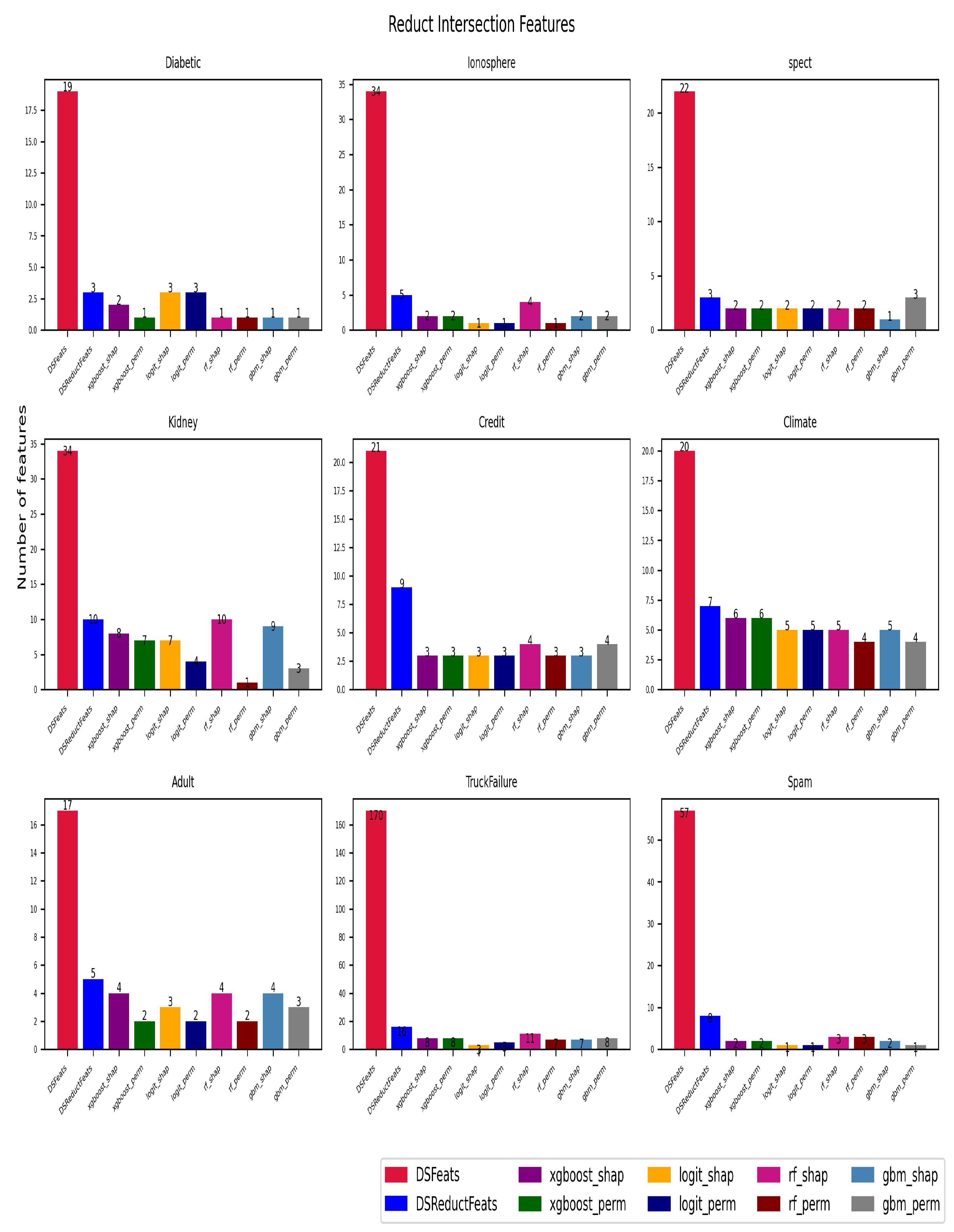
6.1. Experimental Results

The results of the experiments are summarized in

Table 4. Intersection sets.

Dataset	#Features at Dataset Reduct	XGBoost		Logit		RF		GBM
		SHAP	Perm	SHAP	Perm	SHAP	Perm	SHAP	Perm
Diabetic	3	2	1	3	3	1	1	1	1
Ionosphere	5	2	2	1	1	4	1	2	2
Spect	3	2	2	2	2	2	2	1	3
Kidney	10	8	7	7	4	10	1	9	3
Credit	9	3	3	3	3	4	3	3	4
Climate	7	6	6	5	5	5	4	5	4
Adult	5	4	2	3	2	4	2	4	3
Truck Failures	16	8	8	3	5	11	7	7	8
Spam	8	2	2	1	1	3	3	2	1

,

Table 5. Reduct ratios: results (rounded to 4 digits).

Dataset	XGBoost		Logit		RF		GBM
	SHAP	Perm	SHAP	Perm	SHAP	Perm	SHAP	Perm
Diabetic	0.3358	0.3333	0.3665	0.3562	0.3333	0.3333	0.3333	0.3333
Ionosphere	0.3382	0.1599	0.0	0.0	0.4329	0.0	0.3945	0.0552
Spect	0.3736	0.3756	0.6099	0.5652	0.5297	0.6291	0.3333	0.362
Kidney	0.4995	0.1983	0.2889	0.1724	0.5473	0.0	0.3905	0.04149
Credit	0.1341	0.1405	0.149	0.113	0.1357	0.1239	0.1423	0.1283
Climate	0.3761	0.3237	0.3408	0.3278	0.3276	0.2695	0.2995	0.3169
Adult	0.3272	0.0508	0.3217	0.2999	0.3159	0.2831	0.4084	0.3949
Truck Failures	0.1237	0.1896	0.0865	0.0718	0.2572	0.0348	0.0517	0.0202
Spam	0.2012	0.1931	0.0175	0.1047	0.2562	0.1659	0.1294	0.1249

,

Table 6. AIC values: results (rounded to 4 digits).

Dataset	XGBoost		Logit		RF		GBM
	SHAP	Perm	SHAP	Perm	SHAP	Perm	SHAP	Perm
Diabetic	3.1804	5.1699	1.3173	1.2706	5.1699	5.1699	5.1699	5.1699
Ionosphere	7.1912	6.5031	8.0	8.0	3.6365	8.0	7.4475	6.1638
Spect	3.3498	3.3587	4.7162	4.4033	4.1767	4.8619	5.1699	1.2969
Kidney	5.9973	6.6378	6.984	12.5459	2.2866	18.0	3.4284	14.1223
Credit	12.4154	12.4368	12.4656	12.345	10.4208	12.381	12.4427	10.3962
Climate	3.3613	3.1287	5.2023	5.1459	5.1452	6.9059	5.0272	7.0998
Adult	3.1435	6.1503	5.1199	7.0289	3.0958	6.9604	3.5144	5.4496
Truck Failures	16.3809	16.6064	26.2609	22.2149	10.8579	18.1023	18.1531	16.0588
Spam	12.6483	12.6191	14.0508	14.3191	10.8541	10.523	12.3999	14.3853

and

Table 7. BIC values: results (rounded to 4 digits).

Dataset	XGBoost		Logit		RF		GBM
	SHAP	Perm	SHAP	Perm	SHAP	Perm	SHAP	Perm
Diabetic	11.0259	20.8609	1.3173	1.2706	20.8609	20.8609	20.8609	20.8609
Ionosphere	26.4699	25.7819	33.7051	33.7051	10.0627	33.7051	26.7263	25.4426
Spect	8.8497	8.8586	10.216	9.9031	9.6765	10.362	16.1696	1.2969
Kidney	18.6411	25.6035	25.9499	50.4775	2.2866	74.8974	9.7504	58.3758
Credit	55.0508	55.0723	55.101	54.9805	45.9503	55.0169	55.0782	45.9257
Climate	8.5312	8.2986	15.5421	15.4858	15.4851	22.4157	15.367	22.6096
Adult	15.6218	43.5855	30.0767	44.4641	15.5742	44.3956	15.9928	30.4064
Truck Failures	110.4675	110.6929	179.1517	151.584	69.662	123.9498	124.0	110.1454
Spam	68.3225	68.2933	79.004	79.2723	57.2492	56.9189	68.0741	79.3385

. Each table comprises nine rows (one for each dataset) and eight columns. For each ML model, there are two columns: the first column represents the results obtained for SHAP, whereas the second column holds the corresponding results for Perm.

As discussed in Section 4, for an XAI method to be selected, this method has to achieve a high reduct ratio, a high number of features in the intersection set, and low AIC and BIC values. Table 4, Table 5, Table 6 and Table 7 highlight the values meeting these prerequisites for each ML model. If both XAI methods achieve the same score, we do not consider any of them to be the best method for the given ML model.

The starting point of our evaluation is the number of features in the intersection set obtained with each XAI method. Table 4 shows the number of features in the reduct of each dataset. Furthermore, for both XAI methods, the respective number of features at the intersection between the XAI method and the dataset reduct is shown. For each XAI method, it has to achieve a number of features as high as possible compared to the value in the first column (dataset reduct). As can be seen, SHAP is scoring better than Perm for most datasets, ignoring cases in which both XAI methods obtain the same scores. SHAP obtains the best scores for all datasets when using it to explain the predictions provided by the RF model. This might indicate that SHAP is able to cope with the randomness in building the RF trees, whereas Perm can not. When explaining GBM predictions, Perm scores better in three datasets, whereas SHAP scores higher in four datasets. Moreover, SHAP performs better for XGBoost, when not considering datasets for which both explainers score the same. When explaining Logit predictions, the results obtained for SHAP and Perm are indecisive for most datasets. However, the number of features captured at the intersection set represents a large percentage of the dataset reduct in all cases. Furthermore, in these datasets when SHAP is scoring better, it can capture most of the features at the reduct of the dataset. Figure 4 plots the volume of the intersection set achieved by both XAI methods when applying them to each of the executed ML models. Figure 4 also plots the total number of features in the dataset as well as the number of features in the respective reduct.

Observation (1): In most cases, SHAP captures a high percentage of the features in the reduct set.

Despite calculating reduct ratios for the features in the intersection sets, the results of reduct ratios do not provide the same indications as in the intersection feature sets results. Table 5 shows the reduct ratios achieved by both XAI methods. As can be seen in the results, SHAP is superior to Perm in almost all ML models executed on all datasets. Perm only scores better for the reduct ratios computed for Spect dataset for three ML models. When SHAP and Perm have the same size of an intersection set, we observe that SHAP is scoring better with respect to the reduct ratios, i.e., the importance score assigned to an intersection feature is higher in the context of SHAP. This difference in the magnitude enabled SHAP to score higher than Perm even though the features in the intersection sets of both XAI methods are similar. Note that this difference in magnitude persists even when normalizing importance scores to fall into the same range.

Observation (2): The difference in magnitude of the importance scores assigned by both XAI methods to the same features is crucial for the computed values of the reduct ratios.

The results of applying the proposed evaluation metrics, i.e., AIC and BIC, are presented in Table 6 and Table 7. For each dataset, we may conclude that the lowest-scoring XAI method is the same in both metrics. Remember that BIC penalizes methods with a low number of features in the intersection set, whereas AIC penalizes methods with a low reduct ratio. A match between the results of both metrics is expected in cases when there is a match between the number of features in the intersection set and the reduct ratio. However, for datasets for which the difference in the reduct ratios between both XAI methods is indecisive, AIC results fluctuate. Figure 5 plots the AIC values we computed for the reduct ratio of both XAI methods. Both AIC and BIC metrics receive the reduct ratios and the number of indispensable features (dataset reduct) that are not present the intersection set of an XAI method. If the difference between the reduct ratios of both XAI methods is unremarkable, we expect that the number of features excluded from the intersection to have a key role in computing AIC values. For these datasets, we believe that computing BIC metric adds more value to the analysis.

Observation (3): AIC and BIC values agree if an XAI method scores higher in terms of the reduct ratio and the number of features in the intersection set. If the reduct ratios are very close, AIC results fluctuate and the BIC metric provides more distinguishing results.

For the RF and GBM models, there is a match between the number of features and the BIC scores. This has been confirmed after analyzing the BIC values and comparing them with the number of features in the intersection sets in Table 4. The XAI method with the lowest number of features excluded from the intersection set (in other words, the highest number of features in the intersection set) scores lower in the BIC metric. If the sizes of intersection sets differ significantly between both XAI methods, this former observation holds. As an example, consider the results of the two XAI methods explaining the predictions of the RF and GBM models. In BIC scores of XAI methods applied to XGBoost and Logit, this observation is true for the datasets for which the number of features at the intersection is different (e.g., in the case of the Diabetic, Kidney, Truck failures, and Adult datasets). The number of features is not a decisive parameter in the remaining five datasets to distinguish between SHAP and Perm when applying them to XGBoost and Logit. In this case, the similarity in the intersection sets and the inconclusive difference between reduct ratios provides room for fluctuation in BIC results and almost similarity as indicated in the results of Credit, Climate, and Spam datasets.

Observation (4): For different sizes of the intersection sets, the BIC measurement can penalize XAI methods with smaller sets. BIC results fluctuate whenever the number of features in the intersection set is similar and the difference between the reduct ratios is unremarkable.

6.2. Discussion

An intersection set with a high number of features indicates the ability of an XAI method to reflect how the ML model uses the indispensable features. However, achieving a high number of features in the intersection sets might not guarantee achieving a high reduct ratio. In a situation for which the dataset reduct is small compared to the complete set of features, the intersection set does not provide a decisive factor to choose either XAI method. Note that this indicates that the dataset holds a large amount of superfluous data that is of low benefit to the ML model.

When computing the reduct ratios, an XAI method, with a high number of features in the intersection set, scores better than another XAI method with a low number of features. However, whenever both XAI methods have the same sizes of intersection sets, scores of these features play an important role. Regarding the results of the experiments (cf. Section 6.1), the AIC and BIC values used for method selection conform to each other. The latter observation holds whenever the difference in the reduct ratios between the XAI methods is unremarkable.

In future work, we will study the effectiveness of the presented approach when applying it to XAI methods that have been designed to explain the predictions of more complex models, i.e., deep learning ones. This necessitates conucting experiments on larger datasets, as it is not feasible to apply deep learning models on the small datasets under investigation in the course of this study. However, with the current experimental setting, we have provided a proof-of-concept of the proposed approach and obtained insightful observations that demonstrate the applicability of the presented approach. To enable further experimentation, extensions, and improvements of the approach, we make the code of these experiments available through our Github https://github.com/GhadaElkhawaga/ConsisXAI (accessed on 27 February 2023).

7. Related Work

With the surge in introducing XAI methods, suitable evaluation metrics are required. There is a lack of objective approaches to functionally evaluate XAI methods [17]. A crucial step in providing such an objective evaluation means of explainability is not only to define how to quantify explainability but also to know which aspects are quantifiable about an explanation. Ref. [38] proposes an approach in which an explainability method is evaluated based on its ability to minimize three complexity measures, i.e., the number of features in an explainer, the interaction strength, and the main effect complexity.

The available objective approaches can be categorized according to the explanation characteristic they address. The Fidelity, stability, and robustness of an XAI method are examples of explanation characteristics that are gaining dedicated attention. There are two reasons that might have contributed to this increased attention. First, these characteristics can be quantified and, hence, triggered more research efforts in proposing metrics for measuring them. Second, the human-independent nature that is associated with these characteristics compared to other characteristics which are subjective in nature. Consider trust and fairness as examples of human-dependent characteristics.

Ref. [39] breaks down XAI effectiveness into four measures which are concerned with the stability of the explanation, the number of features used to build the explanation, the number of rules used in the explanation, and the differing performance between the proxy or interpretable model and the original one. These measures can be translated into the widely quantified XAI characteristics, i.e., fidelity, robustness, and stability. Another evaluation approach is presented in [40], which evaluates the robustness of the explaining technique with respect to changes in the inputs. Ref. [6] proposes a technique to assess the stability of the set of important features and their coefficients which are generated after several runs of the explanation technique, in this case, LIME.

A technique to evaluate the fidelity of XAI methods with respect to black box ML models is presented in [7]. The proposed technique depends on measuring the difference in the predictions between a local XAI method and the original model using perturbed feature vectors instead of the original dataset. Using this technique, Ref. [7] aims to measure the similarity of the decision-making processes of the black box model and the surrogate model trained in the context of the XAI method. An infidelity objective measurement is introduced in [8] to evaluate the expected effect of introducing significant changes to the input to the explanation method on the resulting explanation. By pursuing optimal explanations that decrease the value of infidelity, the robustness of an explanation may be questioned. However, Ref. [8] argues that explanations being highly sensitive to input perturbations are more vulnerable to adversarial attacks, and those with low sensitivity are trivial and vague. Therefore, Ref. [8] proposes a technique that achieves a reduction of sensitivity accompanied by an increase in fidelity. Ref. [9] introduces a method that bases the robustness analysis of an XAI method on feature relevance. Assuming that small perturbations on irrelevant features are not expected to introduce a big change to the output while having the opposite influence on relevant features, Ref. [9] mitigates the risk of having biased and inaccurate conclusions when applying large perturbations and removes relevant features. Thus, it is two-sided in this method where a robustness analysis is not only used to evaluate the quality of an explanation but to also find an important set of features optimizing this measure.

8. Summary and Outlook

Functionally-grounded evaluations of XAI methods aim to measure to what extent an XAI method reflects the relation between the inputs and outputs of a prediction generation process without human involvement. Contemporary proposals to quantitative measurements in the former category mostly target certain explainability characteristics such as fidelity, robustness, and stability of the resulting explanations. In the presented work, we provide an evaluation technique of XAI methods regarding their consistency with ground truth facts. We propose a technique to automatically extract these facts and concepts without predefined parameters or the inclusion of potentially biased techniques. Using the proposed metrics, we quantify the consistency of XAI methods and compared them based on the number of features they extract as well as the reduct ratios.

We applied our proposal to nine publicly available datasets. Our experiments have shown that SHAP performs better in terms of the achieved ratios. Furthermore, SHAP is able to reflect a larger percentage of the underlying concepts in terms of the size of the intersection sets. Computing BIC provides a clear-cut XAI differentiation mechanism if the number of features in the intersection sets differs significantly. Regarding AIC serves the same purpose if there is a difference between the reduct ratios achieved by the different XAI methods. If the difference between the reduct ratios is small, AIC provides information that is redundant to the one achieved through BIC computation. In future work, we want to demonstrate the broad applicability of our approach using more types of predictive models to enable the evaluation of more types of XAI methods based on the proposed approach.

References

1. Binder, A.; Montavon, G.; Lapuschkin, S.; Müller, K.R.; Samek, W. Layer-Wise Relevance Propagation for Neural Networks with Local Renormalization Layers. In Proceedings of the Artificial Neural Networks and Machine Learning—ICANN 2016, Barcelona, Spain, 6–9 September 2016; Lecture Notes in Computer Science; Villa, A.E., Masulli, P., Pons Rivero, A.J., Eds.; Springer International Publishing: Cham, Switzerland, 2016; Volume 9887, pp. 63–71. [Google Scholar] [CrossRef] [Green Version]
2. Ribeiro, M.T.; Singh, S.; Guestrin, C. Why Should I Trust You? In Proceedings of the 22nd ACM SIGKDD International Conference on Knowledge Discovery and Data Mining, San Francisco, CA, USA, 13–17 August 2016; Krishnapuram, B., Shah, M., Smola, A., Aggarwal, C., Shen, D., Rastogi, R., Eds.; ACM: New York, NY, USA, 2016; pp. 1135–1144. [Google Scholar] [CrossRef]
3. Lundberg, S.; Lee, S. A unified approach to interpreting model predictions. In Proceedings of the 31st International Conference on Neural Information Processing Systems (NIPS’17), Long Beach, CA, USA, 4–9 December 2017; Curran Associates Inc.: New York, NY, USA, 2017; pp. 4768–4777. [Google Scholar]
4. Apley, D.; Zhu, J. Visualizing the effects of predictor variables in black box supervised learning models. J. R. Stat. Soc. B 2020, 82, 1059–1086. [Google Scholar] [CrossRef]
5. Kindermans, P.J.; Hooker, S.; Adebayo, J.; Alber, M.; Schütt, K.T.; Dähne, S.; Erhan, D.; Kim, B. The (Un)reliability of Saliency Methods. In Explainable AI: Interpreting, Explaining and Visualizing Deep Learning; Lecture Notes in Computer Science; Samek, W., Montavon, G., Vedaldi, A., Hansen, L.K., Müller, K.R., Eds.; Springer International Publishing: Cham, Switzerland, 2019; Volume 11700, pp. 267–280. [Google Scholar] [CrossRef] [Green Version]
6. Visani, G.; Bagli, E.; Chesani, F.; Poluzzi, A.; Capuzzo, D. Statistical stability indices for LIME: Obtaining reliable explanations for machine learning models. J. Oper. Res. Soc. 2021, 2, 91–101. [Google Scholar] [CrossRef]
7. Velmurugan, M.; Ouyang, C.; Moreira, C.; Sindhgatta, R. Evaluating Fidelity of Explainable Methods for Predictive Process Analytics. In Intelligent Information Systems; Lecture Notes in Business Information Processing; Nurcan, S., Korthaus, A., Eds.; Springer International Publishing: Cham, Switzerland, 2021; Volume 424, pp. 64–72. [Google Scholar] [CrossRef]
8. Yeh, C.K.; Hsieh, C.Y.; Suggala, A.; Inouye, D.I.; Ravikumar, P.K. On the (In)fidelity and Sensitivity of Explanations. Adv. Neural Inf. Process. Syst. 2019, 32. [Google Scholar]
9. Hsieh, C.; Yeh, C.K.; Liu, X.; Ravikumar, P.; Kim, S.; Kumar, S.; Hsieh, C. Evaluations and Methods for Explanation through Robustness Analysis. In Proceedings of the 9th International Conference on Learning Representations, Virtual, 3–7 May 2021. [Google Scholar]
10. Carvalho, D.V.; Pereira, E.M.; Cardoso, J.S. Machine Learning Interpretability: A Survey on Methods and Metrics. Electronics 2019, 8, 832. [Google Scholar] [CrossRef] [Green Version]
11. Guidotti, R.; Monreale, A.; Ruggieri, S.; Turini, F.; Giannotti, F.; Pedreschi, D. A Survey of Methods for Explaining Black Box Models. ACM Comput. Surv. 2019, 51, 1–42. [Google Scholar] [CrossRef] [Green Version]
12. Vilone, G.; Longo, L. Notions of explainability and evaluation approaches for explainable artificial intelligence. Inf. Fusion 2021, 76, 89–106. [Google Scholar] [CrossRef]
13. Jesus, S.; Belém, C.; Balayan, V.; Bento, J.; Saleiro, P.; Bizarro, P.; Gama, J. How can I choose an explainer? In Proceedings of the 2021 ACM Conference on Fairness, Accountability, and Transparency, Virtual, 3–10 March 2021; ACM: New York, NY, USA, 2021; pp. 805–815. [Google Scholar] [CrossRef]
14. Barredo Arrieta, A.; Díaz-Rodríguez, N.; Del Ser, J.; Bennetot, A.; Tabik, S.; Barbado, A.; Garcia, S.; Gil-Lopez, S.; Molina, D.; Benjamins, R.; et al. Explainable Artificial Intelligence (XAI): Concepts, taxonomies, opportunities and challenges toward responsible AI. Inf. Fusion 2020, 58, 82–115. [Google Scholar] [CrossRef] [Green Version]
15. Zhou, J.; Gandomi, A.H.; Chen, F.; Holzinger, A. Evaluating the Quality of Machine Learning Explanations: A Survey on Methods and Metrics. Electronics 2021, 10, 593. [Google Scholar] [CrossRef]
16. Belle, V.; Papantonis, I. Principles and Practice of Explainable Machine Learning. Front. Big Data 2021, 4, 688969. [Google Scholar] [CrossRef]
17. Doshi-Velez, F.; Kim, B. Towards A Rigorous Science of Interpretable Machine Learning. arXiv 2017, arXiv:1702.08608. [Google Scholar] [CrossRef]
18. Bolón-Canedo, V.; Sánchez-Maroño, N.; Alonso-Betanzos, A. A review of feature selection methods on synthetic data. Knowl. Inf. Syst. 2013, 34, 483–519. [Google Scholar] [CrossRef]
19. Jovic, A.; Brkic, K.; Bogunovic, N. A review of feature selection methods with applications. In Proceedings of the 2015 38th International Convention on Information and Communication Technology, Electronics and Microelectronics (MIPRO), Opatija, Croatia, 25–29 May 2015; pp. 1200–1205. [Google Scholar] [CrossRef]
20. Chandrashekar, G.; Sahin, F. A survey on feature selection methods. Comput. Electr. Eng. 2014, 40, 16–28. [Google Scholar] [CrossRef]
21. Balogun, A.O.; Basri, S.; Mahamad, S.; Abdulkadir, S.J.; Almomani, M.A.; Adeyemo, V.E.; Al-Tashi, Q.; Mojeed, H.A.; Imam, A.A.; Bajeh, A.O. Impact of Feature Selection Methods on the Predictive Performance of Software Defect Prediction Models: An Extensive Empirical Study. Symmetry 2020, 12, 1147. [Google Scholar] [CrossRef]
22. Pawlak, Z. Rough Sets: Theoretical Aspects of Reasoning about Data; Theory and Decision Library D; Springer: Dordrecht, The Netherlands, 1991; Volume v.9. [Google Scholar]
23. Molnar, C. Interpretable Machine Learning: A Guide for Making Black Box Models Explainable. 2020. Available online: https://christophm.github.io/interpretable-ml-book/ (accessed on 27 February 2023).
24. Elkhawaga, G.; Abuelkheir, M.; Reichert, M. XAI in the Context of Predictive Process Monitoring: An Empirical Analysis Framework. Algorithms 2022, 15, 199. [Google Scholar] [CrossRef]
25. Akaike, H. A new look at the statistical model identification. IEEE Trans. Autom. Control 1974, 19, 716–723. [Google Scholar] [CrossRef]
26. Vrieze, S.I. Model selection and psychological theory: A discussion of the differences between the Akaike information criterion (AIC) and the Bayesian information criterion (BIC). Psychol. Methods 2012, 17, 228–243. [Google Scholar] [CrossRef] [Green Version]
27. Pedregosa, F.; Varoquaux, G.; Gramfort, A.; Michel, V.; Thirion, B.; Grisel, O.; Blondel, M.; Prettenhofer, P.; Weiss, R.; Dubourg, V.; et al. Scikit-learn: Machine Learning in Python. J. Mach. Learn. Res. 2011, 12, 2825–2830. [Google Scholar]
28. Dua, D.; Graff, C. UCI Machine Learning Repository. 2019. Available online: http://archive.ics.uci.edu/ml (accessed on 27 February 2023).
29. Maalouf, M. Logistic regression in data analysis: An overview. Int. J. Data Anal. Tech. Strateg. 2011, 3, 281–299. [Google Scholar] [CrossRef]
30. Friedman, J.H. Greedy Function Approximation: A Gradient Boosting Machine. Ann. Stat. 2001, 29, 1189–1232. [Google Scholar] [CrossRef]
31. Chen, T.; Guestrin, C. XGBoost: A Scalable Tree Boosting System. In Proceedings of the 22nd ACM SIGKDD International Conference on Knowledge Discovery and Data Mining, San Francisco, CA, USA, 13–17 August 2016; ACM: New York, NY, USA, 2016; pp. 785–794. [Google Scholar] [CrossRef] [Green Version]
32. Breiman, L. Random Forests. Mach. Learn. 2001, 45, 5–32. [Google Scholar] [CrossRef] [Green Version]
33. Raileanu, L.E.; Stoffel, K. Theoretical Comparison between the Gini Index and Information Gain Criteria. Ann. Math. Artif. Intell. 2004, 41, 77–93. [Google Scholar] [CrossRef]
34. Urbanowicz, R.J.; Meeker, M.; La Cava, W.; Olson, R.S.; Moore, J.H. Relief-based feature selection: Introduction and review. J. Biomed. Inform. 2018, 85, 189–203. [Google Scholar] [CrossRef] [PubMed]
35. Zdravevski, E.; Lameski, P.; Kulakov, A. Weight of evidence as a tool for attribute transformation in the preprocessing stage of supervised learning algorithms. In Proceedings of the 2011 International Joint Conference on Neural Networks, San Jose, CA, USA, 31 July–5 August 2011; pp. 181–188. [Google Scholar] [CrossRef]
36. Cao, R.; González Manteiga, W.; Romo, J. Nonparametric Statistics; Springer International Publishing: Cham, Switzerland, 2016; Volume 175. [Google Scholar] [CrossRef] [Green Version]
37. Lindman, H.R. Analysis of Variance in Experimental Design; Springer Texts in Statistics; Springer: New York, NY, USA, 1992. [Google Scholar] [CrossRef]
38. Molnar, C.; Casalicchio, G.; Bischl, B. Quantifying Model Complexity via Functional Decomposition for Better Post-hoc Interpretability. In Communications in Computer and Information Science. Machine Learning and Knowledge Discovery in Databases; Cellier, P., Driessens, K., Eds.; Springer: Cham, Switzerland, 2020; Volume 1167, pp. 193–204. [Google Scholar] [CrossRef] [Green Version]
39. Rosenfeld, A. Better Metrics for Evaluating Explainable Artificial Intelligence. In Proceedings of the AAMAS ’21: Proceedings of the 20th International Conference on Autonomous Agents and MultiAgent Systems, Online, 3–7 May 2021; pp. 45–50. [Google Scholar]
40. Alvarez-Melis, D.; Jaakkola, T.S. On the Robustness of Interpretability Methods. arXiv 2018, arXiv:1806.08049. [Google Scholar]
Figure 1. Categorisation of XAI methods.
Electronics 12 01670 g001
Figure 2. Categories of feature selection methods.
Electronics 12 01670 g002
Figure 3. Proposed approach.
Electronics 12 01670 g003
Figure 4. Number of features in the intersection sets obtained by each XAI method.
Electronics 12 01670 g004
Figure 5. AIC values obtained at each reduct ratio.
Electronics 12 01670 g005