1. Introduction
Cold-rolled strips are widely used in the fields of automobile manufacturing, aerospace, household appliance panels, and so on [
1], because of their high geometric accuracy and great mechanical properties. With the development of technology, cold-rolled strips have become thinner and thinner, and the geometric shape and dimensional accuracy requirements are becoming higher and higher [
2,
3]. In order to improve the quality of the strips, modern rolling mills adopt an automatic gauge control system (AGC) to solve the gauge problem, and an automatic flatness control system (AFC) to solve the flatness problem. At present, the gauge control basically meets the requirements, but the flatness problem is becoming more and more complicated [
4]. Due to the large number of actuators required for flatness control, and the strong coupling and hysteresis between the actuators [
5], flatness control is still a great challenge in practice. The cold tandem rolling mill contains multi-stand flatness controls, and the final stand is a closed-loop feedback control. The control efficiency reflects the adjustment ability of the actuators to the flatness in a closed-loop feedback control. Distributing the flatness deviation to each actuator reasonably can improve the flatness control accuracy [
6]. In actual production, the control efficiency of each actuator varies with different process parameters, especially, when the ratio of the width to thickness is larger, it is more unstable. The control efficiency is often obtained by an empirical method which has been used since setting up the factory. However, there are errors, inevitably, for specific working conditions, and the update speed is slow. Therefore, obtaining an accurate control efficiency is significant in the research on flatness control.
To the best of our knowledge, there are two main methods used to obtain the control efficiency: the experimental method and the finite element method [
7]. The experimental method obtains the control efficiency by changing the setting value of the actuator one by one to obtain the change of the flatness. Although it is more accurate, the high cost and the limited working conditions make it infeasible. Compared with the experimental method, the finite element simulation has the advantage of being more economical, having a wider application, and more flexible simulation of various rolling conditions [
8]. However, the finite element method needs many assumptions in the analysis of the rolling process, which leads to errors between the calculation results and the actual situations. Meanwhile, the calculation process is slow, so it is not suitable for the requirements of online real-time control [
9]. Thanks to a large amount of rolling process data stored by steel companies, a lot of information related to the production process can be revealed with the development of big data and sensor technology [
10]. However, the use of the rolling process data is not sufficient. Therefore, based on the rolling process data, mining the information with the goal of analyzing the relationship between the flatness and the process, provides not only a new way to improve the flatness control accuracy but also a new approach for the intelligent recognition of the flatness control efficiency.
The actual rolling production data has the characteristics of noise, outliers, deviations, and so on. In order to calculate the control efficiency, it is necessary to analyze and process the data. Thus, it is extremely important to reduce the noise of the production data. Wavelet transform, a key noise reduction method at home and abroad, has the advantages of multi-resolution, fast operation speed and small storage space. In addition, it has been widely used in the fields of image compression, data denoising, and edge detection.
Y. Kim et al. proposed cepstrum-assisted empirical wavelet transform (CEWT) to decompose the signal in the fault diagnosis of planetary gear trains. The CEWT solved the problem of empirical wavelet transform (EWT), which required physical understanding to isolate fault-related signals and improve performance of fault diagnosis [
11]. F. Dengand et al. proposed a new peak detection algorithm based on continuous wavelet transform and image segmentation, which has made progress in identifying weak peaks, overlapping peaks, and removing false peaks [
12].
M. Zolfaghari found that the electricity production data in the prediction is non-stationary and non-linear, and traditional forecasting methods display a poor robustness. Therefore, they proposed an AWT-LSTM-RF hybrid model, combining adaptive wavelet transform (AWT), long short-term memory network (LSTM), and random forest (RF) algorithms for the prediction. The results showed that the hybrid model of AWT-LSTM-RF is better than the benchmark model. At the same time, the wavelet transform algorithm for the treatment of the input data can improve the predictive ability of RF [
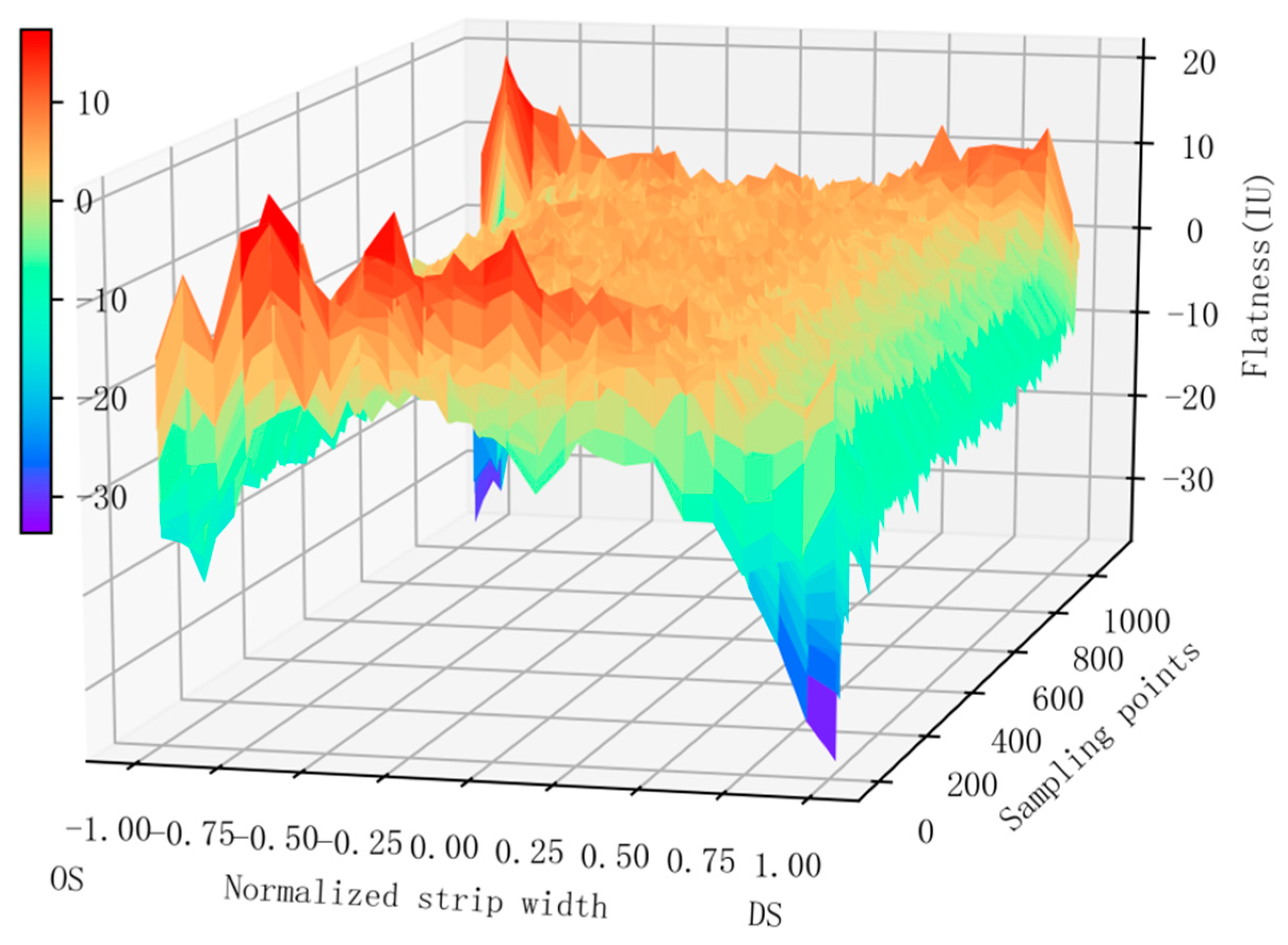
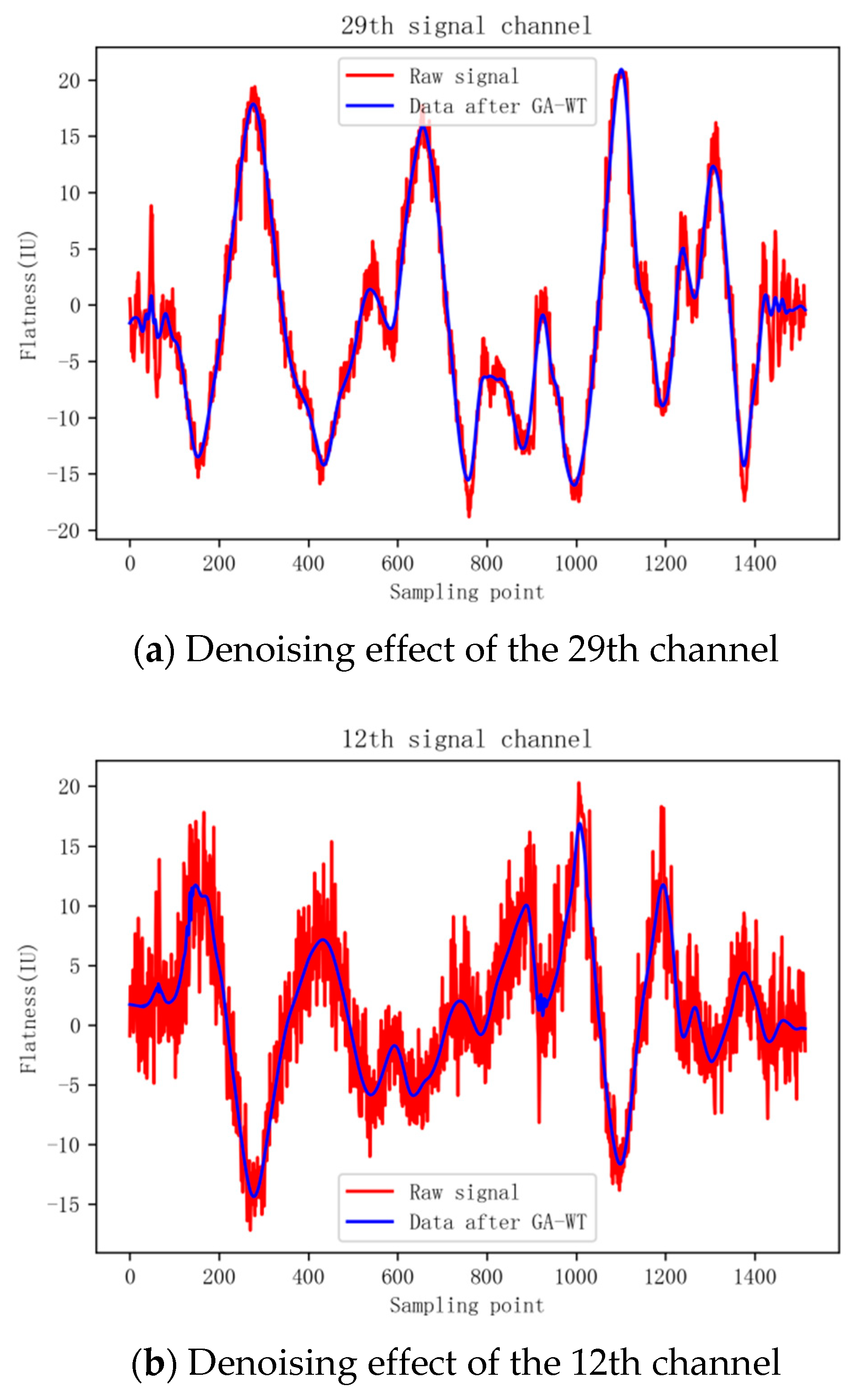
13]. Denoising the actual data under the wavelet transform alone leads to signal distortion, therefore, the threshold of wavelet coefficients can be optimized in combination with the genetic algorithm, to remove noise as much as possible while retaining the characteristics of the signal. The flatness meter has dozens of sensor channels and these sensor channels can measure the flatness along the width direction at the same time.
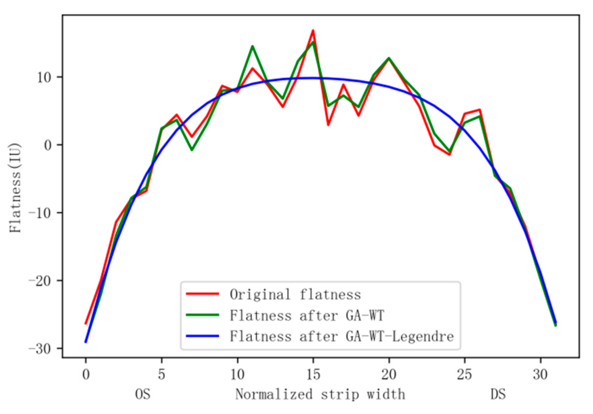
Figure 1 shows the measurement signal of the strip flatness coil. Because of the noise interference in the actual signal, the characteristics of the flatness cannot be expressed directly. Therefore, data processing is required. Simply denoising each signal channel can only solve the noise problem of a single sensor channel, and the strip flatness represented by the width direction sensor still has no obvious strip flatness features. So it is necessary to fit in the width direction with a Legendre orthogonal polynomial to obtain the strip flatness represented by the width direction sensor signal. Based on the strip flatness features extracted after denoising, Legendre fitting, and the corresponding actual production process data, an optimized algorithm is used to intelligently identify the strip flatness control effect. The Adam optimization algorithm is an extension of the stochastic gradient descent method. It has the advantages of simplicity, directness, high efficiency, small memory, and handling sparse gradients in solving non-convex optimization problems.
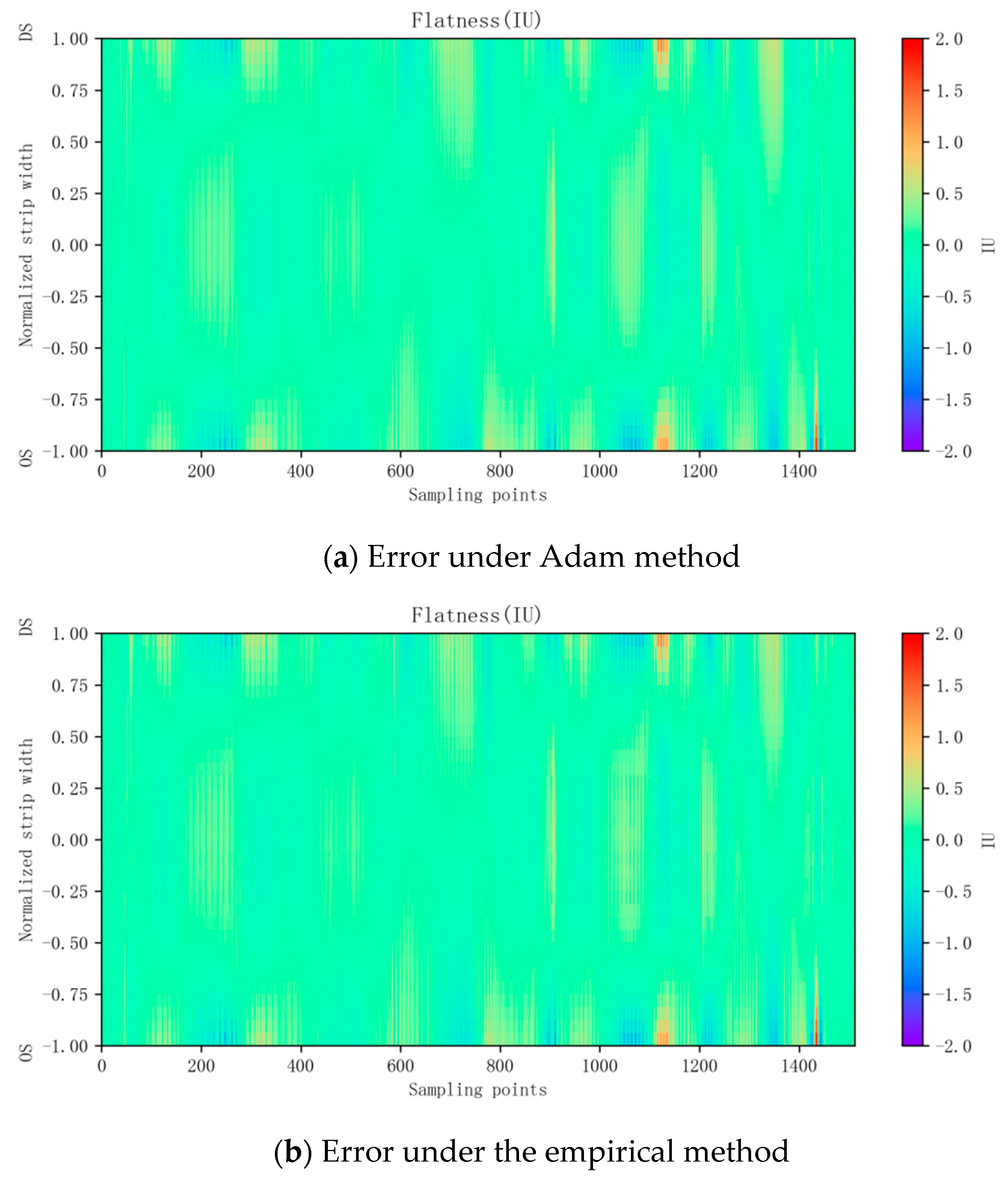
This work chooses the Adam optimization method to identify the flatness control efficiency. Based on the actual production process data of a tandem cold rolling mill, the influence of the different actuators on the flatness is analyzed. The GA-WT-Legendre-Adam intelligent identification method for flatness adjustment and control effects is proposed and compared with the control efficiency determined by the empirical method. The analysis results show that the method proposed in this paper can effectively reduce the influence of noise, and the flatness residual MSE calculated by the recognized flatness control efficiency is reduced by 5.4% compared with the empirical method. This noise reduction method can use the industrial data of online production to realize the online identification of the flatness control efficiency.
2. Flatness Closed-Loop Control System
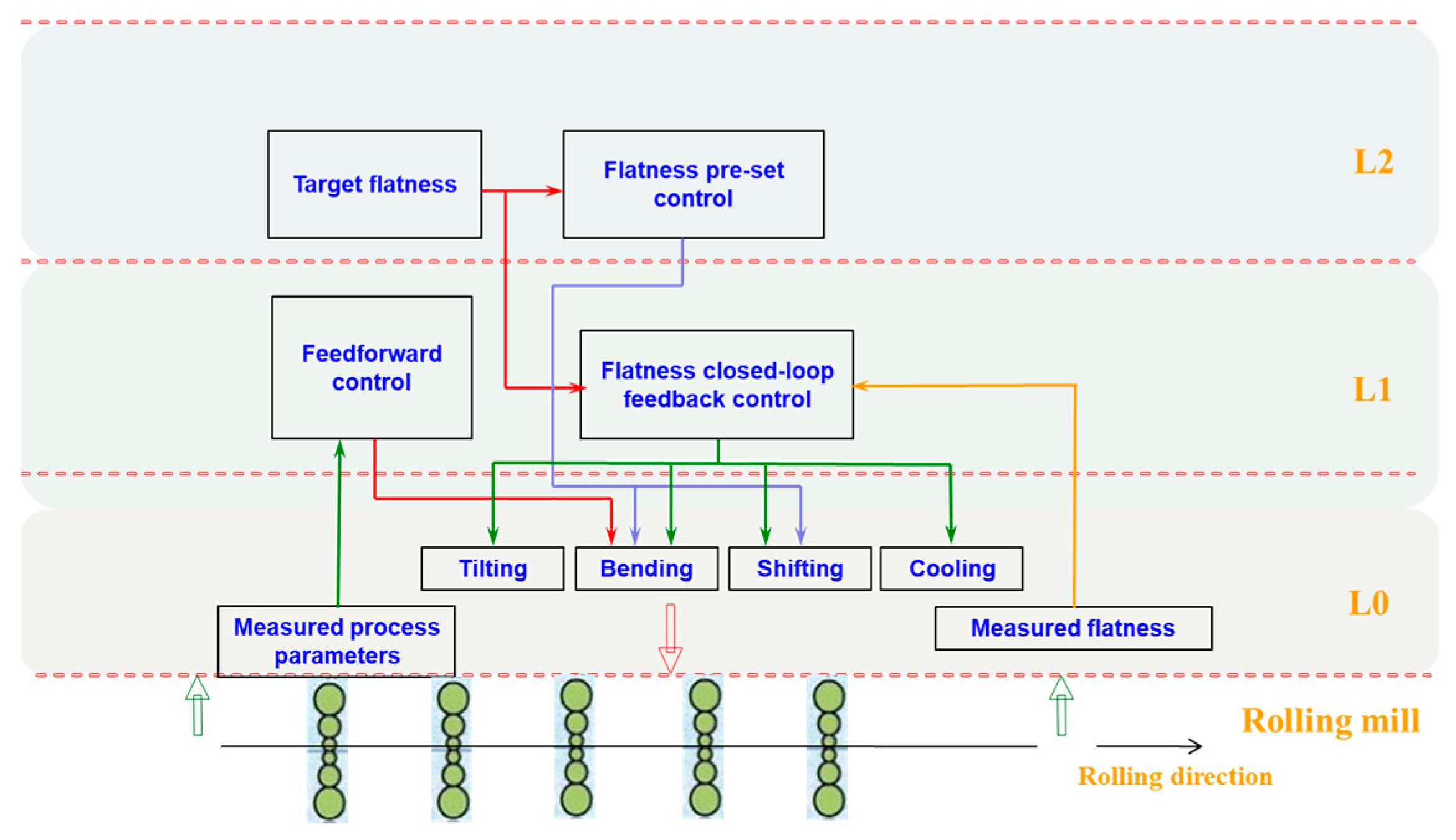
A cold tandem rolling mill consists of a five-stands six-high UCM (Universal Crown Mill). Among them, the first four stands use a preset model to make preliminary adjustments to the thickness and flatness of the strip. The fifth stand uses a closed-loop feedback control strategy to adjust the flatness, which is the most critical part in the flatness control system. The flatness control system is shown in
Figure 2. The flatness closed-loop feedback control system is established in the rolling stabilization stage. The closed-loop feedback control model calculates the adjustment of the actuator through the deviation between the measured flatness and the target flatness. Then a control signal is sent to the actuator and the new flatness deviation is detected at the same time. Continuous dynamic adjustments for the actuator in real time are essential for obtaining a stable and good flatness [
14,
15]. At present, the five-stands cold tandem rolling mill includes intermediate roll bending (IRB), intermediate roll shifting (IRS), work roll bending (WRB), tilting and segment cooling, and other actuators [
16,
17]. Among them, tilting can eliminate the first order flatness deviation. WRB, IRB, and IRS can eliminate the secondary and the fourth order flatness deviations. Elimination of the higher order flatness deviation requires segmented cooling [
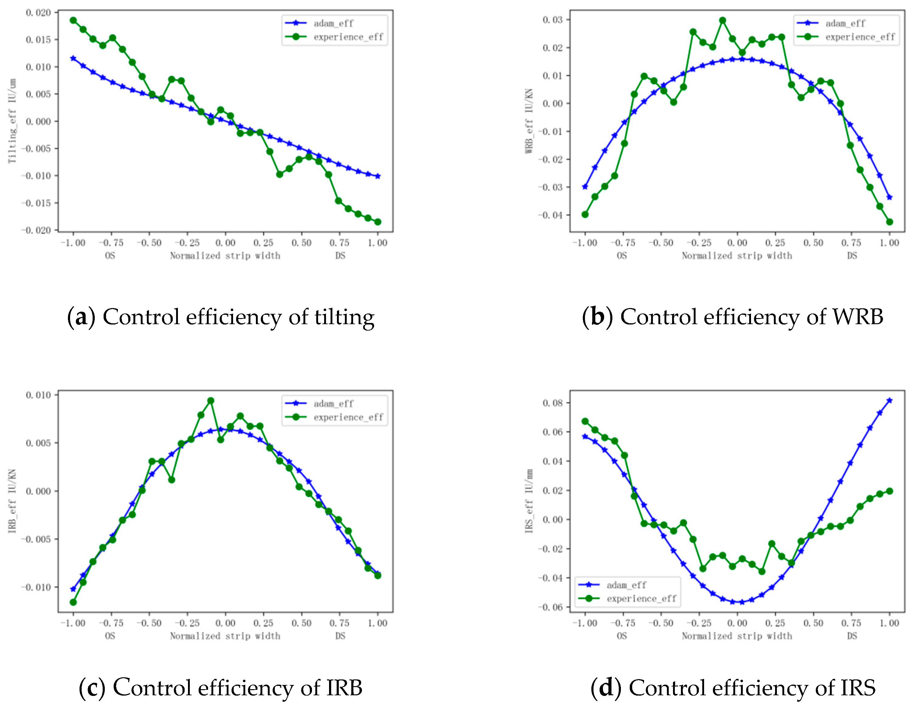
18]. The control performance of each type of actuator can be reflected on the control efficiency curve. The general segmented cooling of work rolls cannot be solved by formulas, and the response speed is slow. It is often used to eliminate the remaining flatness deviation after the adjustment of other actuators. Therefore, this paper only takes the influence of tilting, WRB, IRB, and IRS into account.
The basis of the flatness control is the control efficiency, which can effectively reflect the control performance of the actuators on the flatness. Because of its simplicity and fast calculation process, it can play a key role in a unit with a variety of control methods. The control efficiency can be optimized by making full use of the rolling production process data to obtain a more precise flatness control [
19]. The control efficiency, described by the following Formula (1), means the change of the flatness deviation caused by the change of each unit of the actuator:
where
is the actuator efficiency of the
th actuator in the
th segment of the width direction,
is the adjustment of the
jth actuator and
is the flatness change caused by the
th actuator in the
th segment of the width direction.
The multi-variable optimal flatness control algorithm, based on control efficiency, studies the effect of the actuator on the flatness deviation of each measurement section in the width direction. The control amount of each actuator can be solved in connection with the flatness deviation of each measurement section to get the optimal control for the entire system. Therefore, as long as the control efficiency of the flatness is obtained, the adjustment of each actuator under the optimal flatness control can be calculated using Formula (2), to guarantee the minimum value of the performance index
J.
is the target flatness deviation in the th segment of the width direction, is the number of flatness control technologies, and is the number of flatness measurement channels in the width direction.
Among the required actuators, the response speed of the tilting is the fastest, which mainly eliminates the asymmetric flatness deviation, so the control strategy mainly refers to the control of the roll bending and roll shifting. Due to the large number of different control methods, various control goals and the coupling effects of them, choosing either the sequential or parallel calculation needs to be considered for adjustment in the flatness control. The cold tandem rolling mill that provides the data source for this paper adopts a sequential solution strategy, also known as a relay solution, which is based on the least squares principle of the priority sequence table. The execution mechanism is calculated hierarchically based on the sequence in the priority sequence table. The objective function of an executive agency can be expressed as
where
is the objective function of the
jth actuator;
is the remaining flatness deviation after the adjustment of the first
actuators.
In order to minimize the objective function
, the partial derivative of the objective function is calculated, as in Equation (4), to obtain the adjustment of the
jth actuator.
The priority is determined by the sensitivity of the actuator. Generally, it has the sequence of WRB, IRB, and IRS. The sequential solution strategy makes the best use of the actuators to eliminate the flatness deviation. When the front actuator cannot completely eliminate the flatness deviation, the remaining flatness deviation is eliminated by the latter actuator. Because this kind of control strategy calculates the control quantity of each actuator in sequence, according to the artificially prescribed sequence, there is no unsolvable situation. It successfully avoids the matrix solving process and the limit problem of the actuator, which are not suitable for online and real-time use. From the above calculation formula, it is obvious that accurate control efficiency is the core content of the flatness closed-loop control system, which is different from the empirical method that has a long update cycle and is not suitable for specific working conditions. The data-driven method can dynamically obtain the flatness control functions of different steel specifications from the data more accurately and with a greater flexibility, thereby the accuracy of the closed-loop feedback control of the current steel specifications can be improved.
3. Establishment and Test of Noise Reduction Model
Using actual production data to establish a data-driven model for the intelligent recognition of the flatness control efficiency can reflect the real performance of the flatness control mechanism, and realize the adjustment of the control efficiency with the change of working conditions. However, the data actually collected at the production site contains noise, has a wide range of fluctuations, and thus the true situation of the data is obscured. It is necessary first to extract meaningful flatness features to establish a data-driven intelligent identification model of flatness control efficiency.
Wavelet transform is a time-frequency localization analysis method, in which the wavelet window area is constant and the time and frequency domain window ranges are variable. It solves the shortcoming of the short-time Fourier transform, which adopts a fixed sliding window function and cannot change the time resolution. Wavelet transform uses a short-time window when analyzing high-frequency signals and a long-time window when analyzing low-frequency signals. This achieves the adaptive change of the time-frequency window and has the abilities of local analysis and refinement.
The wavelet of continuous wavelet transform is a short-duration time function. Suppose that
is an integrable function and
.
is a basic wavelet or wavelet mother function, if the Fourier transform satisfies:
By shifting and scaling the wavelet
, a set of wavelet basis functions
can be obtained:
where
and
.
b is the translation factor indicating the position where the function is translated along the
t axis and
a is the scale factor of a wavelet basis function.
For a signal
, its continuous wavelet transform is:
where
is the coefficient after wavelet transform of the signal
. Through the inverse transform of
, we can obtain:
In practical applications, the wavelet transform needs to be discretized. Generally, the scale factor and translation factor of the continuous wavelet transform are discretized. The scale factor is
and the translation factor is
,
. The step value is a fixed value other than 1, and usually
, then the function can be written as
The corresponding discrete wavelet transform can be written as
Because the wavelet transform has the characteristics of multi-resolution, it can effectively remove the noise while preserving the characteristic information of the original signal as much as possible. The formula for wavelet denoising is as follows:
where
is the actual noisy signal,
is the effective signal,
is the sampling time,
is the noise intensity and
is the noise component.
Wavelet denoising requires processes such as multi-layer decomposition of noisy signals, threshold processing of wavelet coefficients, and reconstruction of the wavelet inverse transform. The more decomposition layers of a noisy signal there are, the easier it is to eliminate the noise signal, but the error is greater after reconstruction. So it is very important to choose an appropriate number of decomposition layers. The appropriate number of decomposition layers can be calculated using Formula (12):
where
is the number of decomposition levels,
is the length of the data, and
is the length of the filter.
The processing of the wavelet coefficient threshold is a key factor to improve the effect of wavelet denoising. Common threshold functions include the hard threshold and the soft threshold. Since the soft threshold function can shrink large coefficients, it can reduce the discontinuity problems in the hard threshold noise reduction process. At the same time, it has a good adaptability and an excellent noise reduction effect. Therefore, the soft threshold function is selected in this paper as follows:
where
is the wavelet coefficient,
is the threshold, and
is the wavelet coefficient after threshold processing.
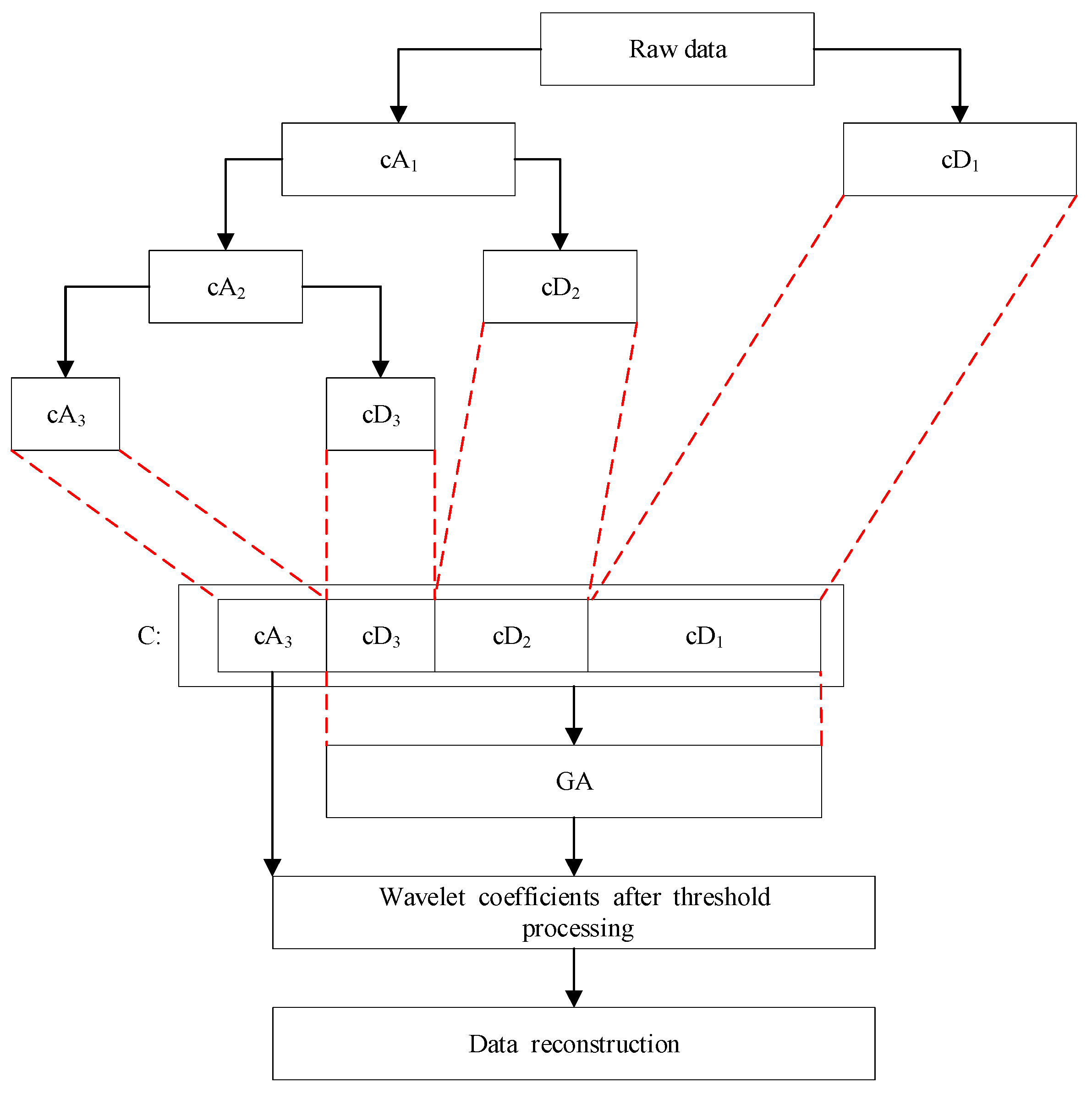
From (13), it can be found that, how to choose an appropriate threshold is the key to wavelet denoising. In order to obtain the optimal wavelet coefficients, this paper combines a genetic algorithm to optimize the threshold. After the wavelet coefficients are decomposed by the wavelet transform, the genetic algorithm is used to select an appropriate threshold, remove the noise in the high frequency, and retain the useful information. Then the wavelet inverse transform is reconstructed to obtain the noise-reduced data.
Figure 3 shows the noise reduction process of GA-WT (Genetic Algorithm-Wavelet).
To establish the GA-WT model, it is necessary to select an appropriate wavelet basis function. In this paper, the db8 basis function is selected, and the number of decomposition layers calculated by Formula (12) is six. The low-frequency wavelet coefficients are reserved, and the optimal threshold is selected by the genetic algorithm for high-frequency wavelet coefficients. The initial population of the genetic algorithm is 200, the crossover probability is 0.8, the number of iterations is 50, and the mutation probability is 0.003.
In order to verify the performance of the model, a standard data set is established. White noise is added to obtain simulation data. The commonly used EEMD (Ensemble Empirical Mode Decomposition) noise reduction method, and the wavelet transform method without genetic algorithm optimization, are compared with the GA-WT method proposed in this paper. The Signal to Noise Ratio (SNR) and Root Mean Square Error (RMSE) are used to measure the noise reduction performances of these three methods. The SNR is defined as the ratio of the effective component of the reconstructed signal to the noise. A larger ratio indicates a better noise reduction performance. The calculation formula is:
where
is the original signal,
is the signal after denoising, and
is the signal length.
The RMSE reflects the similarity between the reconstructed signal and the original signal. A smaller value of RMSE indicates that the reconstructed signal is closer to the original signal. It is defined as:
According to the GA-WT model, the appropriate wavelet basis function needs to be selected firstly. This paper chooses the db8 basis function, and the number of decomposition layers is 6, from Formula (12). The low frequency part is retained, and the genetic algorithm is used to select the optimal soft threshold for the high frequency part.
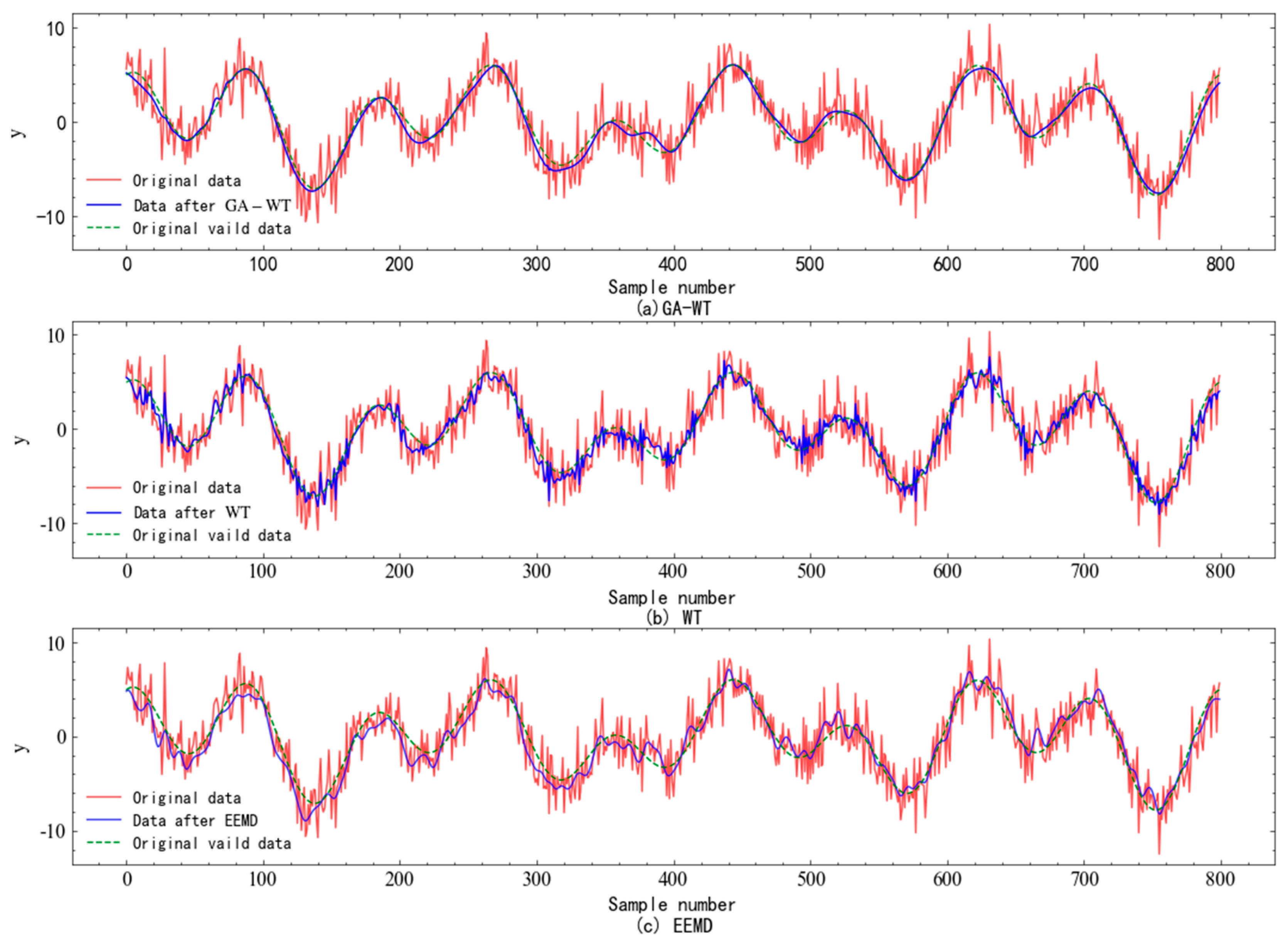
Figure 4 shows the comparison of these three methods before and after denoising. It is obvious that these three methods can basically restore the signal trend. In detail, the wavelet transform based on the genetic algorithm performs better and reconstructs the original data more precisely. The unoptimized wavelet transform and EEMD fluctuate greatly, and the noise is not removed as much as possible. Even some valid information is deleted at the same time.
The SNR comparison of these three methods is shown in
Table 1. The SNR of GA-WT is 18.98 db, which is higher than the 14.41 db of the unoptimized wavelet transform and 12.42 db of EEMD. At the same time, the RMSE of GA-WT is 0.39 IU. This is lower than 0.67 IU of the wavelet transform without optimization and 0.87 IU of EEMD. It shows that the noise reduction performance of GA-WT is the best, so the GA-WT method is chosen in this paper to reduce the noise of the measured flatness data.
5. Conclusions
(1) This paper employs a GA-WT denoising method to deal with the large measurement noise in each signal channel of the flatness meter. Compared with the unprocessed wavelet transform, the SNR of GA-WT is increased by 31.7% and the RMSE is reduced by 41.8%. Compared with EEMD, the SNR of GA-WT is increased by 52.8% and the RMSE is reduced by 55.2%.
(2) GA-WT is used to perform longitudinal denoising in the strip length direction for each signal channel of the flatness meter. Legendre orthogonal polynomial fitting is used on all the flatness signal channels in the width direction, after longitudinal denoising. The method proposed can extract the flatness features, and reflect the real flatness, which can be controlled by the flatness control actuators.
(3) Based on the processed flatness data and the adjustment of the actuator, compared with the empirical method, the control efficiency calculated by the Adam algorithm is 0.035. This is 5.4% lower than the empirical method, which indicates that the GA-WT-Legendre-Adam method can effectively extract flatness features and obtain a more accurate control efficiency.
(4) Production data is characterized by high noise and low quality. In the future, noise reduction and calculation accuracies will be improved further by improving the quality of the actual production data.


