Chattering Free Sliding Mode Control and State Dependent Kalman Filter Design for Underground Gasification Energy Conversion Process

Abstract

The fluctuations in the heating value of an underground coal gasification (UCG) process limit its application in electricity generation, where a desired composition of the combustible gases is required to operate gas turbines efficiently. This shortcoming can be addressed by designing a robust control scheme for the process. In the current research work, a model-based, chattering-free sliding mode control (CFSMC) algorithm is developed to maintain a desired heating value trajectory of the syngas mixture. Besides robustness, CFSMC yields reduced chattering due to continuous control law, and the tracking error also converges in finite time. To estimate the unmeasurable states required for the controller synthesis, a state-dependent Kalman filter (SDKF) based on the quasi-linear decomposition of the nonlinear model is employed. The simulation results demonstrate that despite the external disturbance and measurement noise, the control methodology yields good tracking performance. A comparative analysis is also made between CFSMC, a conventional SMC, and an already designed dynamic integral SMC (DISMC), which shows that CFSMC yields $71.2\%$ and $69.9\%$ improvement in the root mean squared tracking error with respect to SMC and DISMC, respectively. Moreover, CFSMC consumes $97\%$ and $23.2\%$ less control energy as compared to SMC and DISMC, respectively.

1. Introduction

Coal plays a pivotal role in global power generation owing to its affordability and ubiquitous presence worldwide. However, the greenhouse gas emissions due to the combustion of fossil fuels negatively impact the environment and contribute significantly to global warming [1]. These environmental concerns are addressed by employing various clean coal energy technologies, for example, the underground coal gasification (UCG) process, that allows the removal of harmful elements at various stages of the UCG process [2]. UCG process involves drilling two wells from the surface of the earth to the coal beds. The injection well is utilized to inject the oxidants like air and steam into the coal bed. These oxidants then react with the ignited coal, and syngas is produced at the production well [3]. Syngas is a flammable gas comprising of higher hydrocarbons, $\mathrm{CO}$, ${\mathrm{H}}_2$, and ${\mathrm{CH}}_4$, that can be utilized in many applications such as the production of liquid fuel and electric power generation. In comparison to conventional mining and surface gasifiers, UCG provides an efficient and cost-effective solution to produce decarbonized gas without putting human labor in danger underground [4].

Industrial applications like integrated gasification combined cycle turbines (IGCC) efficiently operate on a constant heating value/calorific value of syngas. The desired heating value can be achieved by controlling the flow rate or molar flux of the injected oxidants [5]. The presence of parametric uncertainties, modeling inaccuracies, and external disturbances constitutes a challenging control problem that has recently become an emerging field of research [4].

1.1. Related Work

Both model-free and model-based controllers are designed for a UCG system in the literature, to achieve the desired syngas properties. In [6,7], a conventional Proportional Integral (PI) controller is designed to control the temperature, concentration, and heating value of syngas for a lab scale setup for UCG. This model-free controller solely relies on the output measurements. The authors extended their research work to include the effect of uncertainties in the measurements in [8]. Later, in [9], an experimental study is investigated to solve a real-time optimization problem for the UCG process. The optimal control design technique is used to maximize the $\mathrm{CO}$ concentration in syngas. The authors in [10] conducted an experimental study to achieve the desired calorific value of the syngas by employing an adaptive model predictive control (MPC). In [11], an Internet-of-Things (IoT) based monitoring system is utilized to assist a deep learning-based optimal control technique. In [12], the authors conducted an experimental study to optimize oxygen flow, airflow, and syngas exhaust to maximize the heating value of syngas.

The controllers designed in the literature presented above are either model-free or utilize data-driven modeling techniques. However, model-based control strategies are proven to be more accurate. In this regard, a multitude of research is conducted on various model-based control approaches for the UCG process. In [5], the authors developed a 1-D control-oriented mathematical model of the Thar coal gasifier, which is utilized to design various sliding mode control (SMC) techniques for maintaining a desired level of the heating value. In [13], a time domain UCG process model is developed. The authors also design a conventional SMC for heating value regulation with the assumption that all the state variables are measurable. To remove this discrepancy, [14] employs a gain-scheduled modified Utkin observer (GSMUO) to estimate the unmeasurable states required for designing dynamic SMC. Moreover, a time-varying reference is used to test the performance of the control techniques. Considering the required computational complexity and implementation resources for nonlinear techniques, several linear control techniques are also investigated for the UCG system.

1.2. Gap Analysis

The controllers based on linear models can only work near a particular operating point. To cover the whole operating range between no-load and full load, a robust nonlinear controller is required. The tracking error of the heating value does not converge in finite time for all the aforementioned SMC techniques. However, to cater for the abrupt changes in the demand for electric power, the calorific value of the UCG process also needs to change quickly. Therefore, in an IGCC power plant, a robust and finite time convergent SMC, cf. [15] is required to meet the sudden changes in the electricity demand.

1.3. Major Contributions

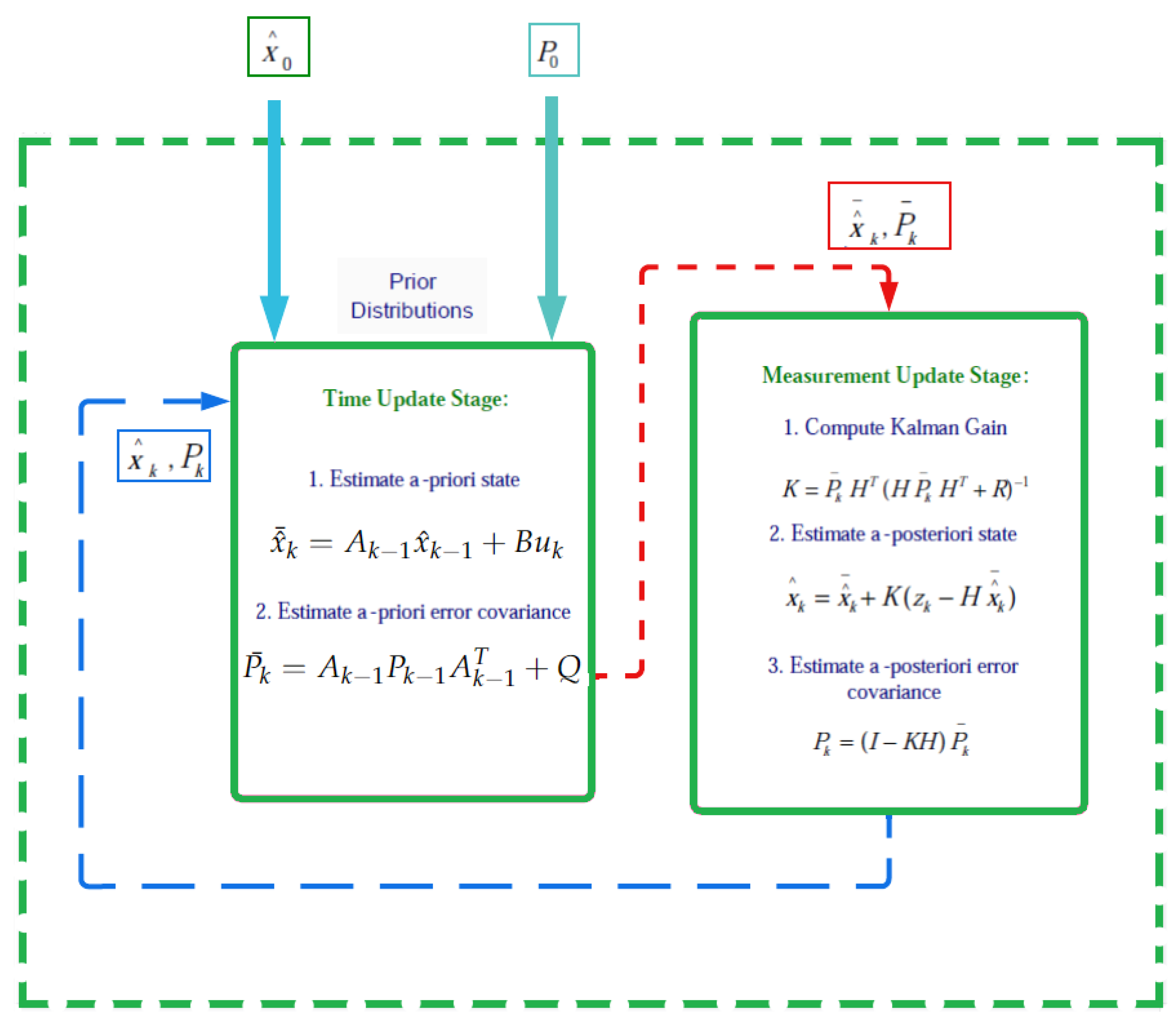
In the current research article, a model-based, chattering-free SMC (CFSMC), cf. [16], is developed for the UCG process model given in [13]. Apart from robustness, CFSMC exhibits less chattering due to continuous control law, and by the virtue of nonlinearity in the sliding surface, the tracking error also converges in finite time. To reconstruct the unmeasurable states necessary for controller design, a state-dependent Kalman filter (SDKF) is designed, which is a linear discrete-time Kalman filter based on the quasilinear model of [13]. The water influx from the surrounding aquifers is considered as the input disturbance, cf. [14], to evaluate the robustness of the control scheme. Furthermore, the performance of the SDKF is evaluated by introducing a measurement noise. Simulation results indicate that the designed methodology quickly and accurately tracks the desired heating value trajectory, outperforming conventional SMC and DISMC (cf. [14]). For brevity, the contributions of the paper are listed below:

• A finite-time CFSMC is designed for the UCG process to track the desired heating value trajectory.
• The unmeasured states used to synthesize the model-based controller are reconstructed using SDKF.
• A thorough quantitative and qualitative comparison is made between the designed technique and already developed techniques for tracking the heating value for the UCG process.

The remaining paper is organized as follows: Section 2 outlines the control-oriented mathematical model of the UCG plant. Section 3 and Section 4 respectively discuss the synthesis of CFSMC and SDKF for the UCG plant. The simulation results are presented in Section 5, followed by the conclusion in Section 6 of the manuscript.

2. Mathematical Model of UCG Process

The current study utilizes a nonlinear control-oriented mathematical model of the UCG process, derived in one of our earlier works [14], for the control design. The mathematical model consists of two solid components: char and coal, and eight gaseous components: ${\mathrm{CO}}_2$, ${\mathrm{O}}_2$, $\mathrm{CO}$, ${\mathrm{H}}_2$, ${\mathrm{CH}}_4$, ${\mathrm{N}}_2$, ${\mathrm{H}}_2\mathrm{O}$, and tar. Moreover, the model incorporates the effect of water influx from the nearby aquifers as the disturbance. The following mathematical equations describe the nonlinear control-oriented UCG model

$$\left.\begin{array}{cc}\hfill {\dot{\rho }}_{Coal}& =-M_1{R}_1,\hfill \\ \hfill {\dot{\rho }}_{Char}& =M_2(0.766R_1-R_2-R_3),\hfill \\ \hfill {\dot{T}}_S& =\frac{1}{C_s}(h_t(T-T_s)-\Delta q_2{R}_2-\Delta q_3{R}_3),\hfill \\ \hfill {\dot{C}}_{CO}& =0.008R_1+R_3-\beta C_{CO},\hfill \\ \hfill {\dot{C}}_{C{O}_2}& =0.058R_1+R_2-\beta C_{C{O}_2},\hfill \\ \hfill {\dot{C}}_{H_2}& =0.083R_1+R_3-\beta C_{H_2},\hfill \\ \hfill {\dot{C}}_{C{H}_4}& =0.044R_1-\beta C_{C{H}_4},\hfill \\ \hfill {\dot{C}}_{Tar}& =0.0138R_1-\beta C_{Tar},\hfill \\ \hfill {\dot{C}}_{H_{2}O}& =0.055R_1+0.075R_2-0.925R_3-\beta C_{H_{2}O}+\frac{\alpha }{L}u+\frac{1}{L}\varphi ,\hfill \\ \hfill {\dot{C}}_{O_2}& =-1.02R_2-\beta C_{O_2}+\frac{\delta }{L}u,\hfill \\ \hfill {\dot{C}}_{N_2}& =-\beta C_{N_2}+\frac{\gamma }{L}u.\hfill \end{array}\right\}$$

(1)

The UCG model includes a number of parameters and variables that are listed in

Table 1. Parameters and states.

Symbol	Description	Unit
$M_i$	Molecular Weight of solids	mol${}^{-1}$ g
T	Temperature of gas	K
$h_t$	Transfer coefficient of heat	cal s${}^{-1}$ K${}^{-1}$ cm${}^{-3}$
$C_s$	Solids specific heat capacity	cal K${}^{-1}$ g${}^{-1}$
R	Chemical reaction rate	mol cm${}^{-3}$ s${}^{-1}$
$\Delta q_i$	Char oxidation heat and steam gasification heat	cal mol${}^{-1}$
L	Reactor’s length	cm
$\beta C_i$	Spatial derivative’s approximation [13]	mol cm${}^{-3}$ s${}^{-1}$
u	Injected gases flow rate	mol cm${}^{-2}$ s${}^{-1}$
$\alpha$, $\delta$, $\gamma$	Amount (%) of $H_{2}O$, $O_2$ and $N_2$ in u	-
$\varphi$	Input disturbance: steam’s flow rate, generated from water influx from nearby aquifers	mol cm${}^{-2}$ s${}^{-1}$

and

Table 2. Nominal parameters value.

${\mathit{C}}_{\mathit{s}}$	$\mathit{\beta }$	P	$h_t$	L	$\Delta q_2$	$\Delta q_3$
7.3920	7 × ${10}^{-6}$	4.83	0.001	100	− 93,929	31,309.7

provides the nominal values of the parameters.

Pyrolysis of coal, oxidation of char, and gasification of steam are dominant chemical reactions of the current model of the UCG process and are expressed in

Table 3. Chemical reactions in UCG.

Sr.	Chemical Equations
$1.$	Coal pyrolysis:
	$C{H}_{0.912}{O}_{0.194}$$\stackrel{R_1}{\to }$$0.766C{H}_{0.15}{O}_{0.02}+0.008CO+0.055H_{2}O+0.083H_2+0.044C{H}_4$ + $0.058C{O}_2+0.0138{\left(C{H}_{2.782}\right)}_9$
$2.$	Char oxidation:
	$C{H}_{0.15}{O}_{0.02}+1.02O_2$$\stackrel{R_2}{\to }$$C{O}_2+0.075H_{2}O$
$3.$	Steam gasification:
	$C{H}_{0.15}{O}_{0.02}+1.02O_2\stackrel{R_3}{\to }CO+H_2$

. Molecular formulas of coal, char and tar are respectively $C{H}_{0.912}{O}_{0.194}$, $C{H}_{0.15}{O}_{0.02}$, and ${\left(C{H}_{2.782}\right)}_9$. The reaction rates of chemical reactions: $R_1$, $R_2$ and $R_3$ are expressed in (2).

$$\left.\begin{array}{cc}\hfill R_1& =5\frac{{\rho }_{coal}}{M_1}exp\left(\frac{-6039}{T_s}\right),\hfill \\ \hfill R_2& =\frac{1}{{\displaystyle \frac{1}{R_{c_2}}}+{\displaystyle \frac{1}{R_{m_2}}}},\hfill \\ \hfill R_3& =\frac{1}{{\displaystyle \frac{1}{R_{c_3}}}+{\displaystyle \frac{1}{R_{m_3}}}},\hfill \end{array}\right\}$$

(2)

where,

$$\begin{array}{cc}\hfill R_{m_2}& =\frac{1}{10}{h}_t{m}_{O_2},\hfill \\ \hfill R_{c_2}& ={\displaystyle \frac{1}{M_2}}\left(9.55\times {10}^8{\rho }_{char}{m}_{O_2}Pexp\left({\displaystyle \frac{-22142}{T_s}}\right)T_s^{-0.5}\right),\hfill \\ \hfill R_{c_3}& ={\displaystyle \frac{{\rho }_{char}{m}_{H_{2}O}^2{P}^{2}exp(5.052-{\displaystyle \frac{12908}{T_s}})}{M_2{\left(m_{H_{2}O}P+exp\left(-22.216+{\displaystyle \frac{24880}{T_s}}\right)\right)}^2}},\hfill \\ \hfill R_{m_3}& =\frac{1}{10}{h}_t{m}_{H_{2}O},\hfill \end{array}$$

the molar fractions $m_{O_2}$ and $m_{H_{2}O}$ are expressed as,

$$\begin{array}{cc}\hfill m_{O_2}& ={\displaystyle \frac{C_{O_2}}{C_T+C_{H_{2}O}}},\hfill \\ \hfill m_{H_{2}O}& ={\displaystyle \frac{C_{H_{2}O}}{C_T+C_{H_{2}O}}},\hfill \end{array}$$

where

$$\begin{array}{cc}\hfill C_T& =C_{CO}+C_{C{O}_2}+C_{H_2}+C_{C{H}_4}+C_{Tar}+C_{O_2}+C_{N_2}.\hfill \end{array}$$

(3)

The nonlinear control-oriented model (1) can be expressed in a control-affine form as

$$\begin{array}{c}\hfill \dot{x}=f\left(x\right)+g_{1}u+g_2\varphi ,\end{array}$$

(4)

where $x\in R^{11}$ is the state vector, u is the control input, $f,g_1,g_2\in R^{11}$ are smooth vector fields, and $\varphi$ is considered as the external disturbance. The vector of states x is chosen as

$$\begin{array}{c}\hfill x={\left[{\rho }_{coal}{\rho }_{char}{T}_s{C}_{CO}{C}_{C{O}_2}{C}_{H_2}{C}_{C{H}_4}{C}_{Tar}{C}_{H_{2}O}{C}_{O_2}{C}_{N_2}\right]}^T.\end{array}$$

(5)

Vector fields $f\left(x\right)$, $g_1$, and $g_2$ are given by (6)–(8), respectively

$$\begin{array}{c}\hfill f\left(x\right)=\left[\begin{array}{c}-M_1{R}_1\left(x\right),\\ M_2(0.766R_1\left(x\right)-R_2\left(x\right)-R_3\left(x\right)),\\ \frac{1}{C_s}(h_t(T-x_3)-\Delta q_2{R}_2\left(x\right)-\Delta q_3{R}_3\left(x\right))\\ 0.008R_1\left(x\right)+R_3\left(x\right)-\beta x_4,\\ 0.058R_1\left(x\right)+R_2\left(x\right)-\beta x_5,\\ 0.083R_1\left(x\right)+R_3\left(x\right)-\beta x_6\\ 0.044R_1\left(x\right)-\beta x_7\\ 0.0138R_1\left(x\right)-\beta x_8\\ 0.055R_1\left(x\right)+0.075R_2\left(x\right)-0.925R_3\left(x\right)-\beta x_9\\ -1.02R_2\left(x\right)-\beta x_{10}\\ -\beta x_{11}\end{array}\right],\end{array}$$

(6)

$$\begin{array}{c}\hfill g_1={\left[\begin{array}{c}00000000\frac{\alpha }{L}\frac{\delta }{L}\frac{\gamma }{L}\end{array}\right]}^T,\end{array}$$

(7)

$$\begin{array}{c}\hfill g_2={\left[\begin{array}{c}00000000\frac{1}{L}00\end{array}\right]}^T.\end{array}$$

(8)

The measurement vector $y_m$ represents the concentration of the gases measured from the gas analyzer

$$\begin{array}{cc}\hfill y_m& ={\left[x_4{x}_5{x}_6{x}_7{x}_8{x}_{10}{x}_{11}\right]}^T,\hfill \end{array}$$

(9)

The heating value $H_v$ of the syngas is the variable to be controlled, characterized as

$$\begin{array}{cc}\hfill H_v& ={\displaystyle \frac{H_4{x}_4+H_6{x}_6+H_7{x}_7}{C_T}},\hfill \end{array}$$

(10)

where $C_T=x_4+x_5+x_6+x_7+x_8+x_{10}+x_{11}$, and $H_4$, $H_6$, and $H_7$ represent heat of combustion (kJ/mol) of $\mathrm{CO}$, ${\mathrm{H}}_2$ and ${\mathrm{CH}}_4$ respectively.

The objective of the control design is to keep the heating value at the desired level based on the operating conditions, such as the usage of char and coal in the UCG bed. Hence, the next section will focus on the design of the controller.

3. Chattering Free Sliding Mode Control Design

This section presents the design of a CFSMC with the aim of following the desired syngas heating value ($H_{vd}$). Despite being a promising solution, the implementation of the sliding mode-based control law may result in high-frequency oscillations, known as chattering, because of modeling errors, external disturbances, and discretization. Chattering is a common issue with sliding mode controllers; however, by the virtue of smoothening terms in the control law and the sliding surface, CFSMC can effectively resolve the issue of chattering [17]. Moreover, a carefully designed sliding surface ensures the finite time convergence of the tracking error. Furthermore, conventional SMC often has the disadvantage of producing discontinuous control inputs that do not meet the requirement of the current system. Therefore, the above-mentioned issues associated with the conventional SMC are addressed in this paper by a systematic design of CFSMC [16].

The output to be controlled is the difference between the actual $H_v$ and its desired trajectory $H_{vd}$, $e=H_v-H_{vd}$. The control input u appears after differentiating e once, which inferred that the relative degree of the tracking error e is 1 with respect to the control input u. Therefore, differentiating the error e with respect to time results in the following error dynamics

$$\begin{array}{c}\hfill \dot{e}=\psi (x,t)+d(x,\varphi ,t)+b(x,t)u,\end{array}$$

(11)

where $\psi (x,t)$, $b(x,t)$, and $d(x,t)$ are smooth and nonlinear functions of states.

It is pertinent to mention here that $\psi (x,t)$ and $b(x,t)$ are the nominal parts of the system, whereas $d(x,\varphi ,t)$ includes the perturbed part of the system influenced by a smooth and bounded input disturbance $\varphi \left(t\right):\left|\varphi \left(t\right)\right|\le {\varphi }_0$. Considering the control-oriented model given in (4) and reaction rate expressions in (2), it can be observed that the input disturbance affects $R_2$ and $R_3$ by changing the concentration of steam. The functions $\psi (x,t)$, $b(x,t)$ and $d(x,t)$ are defined as

$$\begin{array}{cc}\hfill & \psi (x,t)={\displaystyle \frac{C_T(H_4{\dot{x}}_4+H_6{\dot{x}}_6+H_7{\dot{x}}_7)-N(\beta (x_{10}+x_{11})+{\dot{x}}_4+{\dot{x}}_5+{\dot{x}}_6+{\dot{x}}_7+{\dot{x}}_8)}{{C_T}^2}}-{\dot{H}}_{vd},\hfill \\ \hfill & d(x,\varphi ,t)={\displaystyle \frac{(C_T{H}_4+C_T{H}_6-2N){\tilde{R}}_3(x,\varphi )-(1+1.02)N{\tilde{R}}_2(x,\varphi )}{{C_T}^2}},\hfill \\ \hfill & b(x,t)={\displaystyle \frac{-N(\delta +\gamma )}{L{C_T}^2}},\hfill \end{array}$$

(12)

where ${\tilde{R}}_2$ and ${\tilde{R}}_3$ are errors between perturbed and nominal reaction rates, and $N=H_4{x}_4+H_6{x}_6+H_7{x}_7$.

Now, to mitigate error within a finite time, a terminal sliding manifold is chosen for the system in (11) as

$$\begin{array}{c}\hfill S=\dot{e}+csgn\left(e\right){\left|e\right|}^{\lambda },\end{array}$$

(13)

where c and $\lambda$ are design parameters. The value of c is selected such that the polynomial $\rho +c$, which corresponds to the system (13), is Hurwitz, meaning its eigenvalues are in the open left half of the complex plane, with $\rho$ as a Laplace operator. By selecting appropriate values of c and $\lambda$, the ideal sliding mode $S=0$ for the error dynamics (11) can be achieved, resulting in the system converging to its equilibrium point, $e=0$, from any initial condition along the sliding surface $S=0$ in a finite amount of time [16]. Hence, the control law is chosen as

$$\begin{array}{c}\hfill u=-{\displaystyle \frac{1}{b(x,t)}}(u_{eq}+u_{dis}),\end{array}$$

(14)

where

$$\begin{array}{cc}\hfill u_{eq}& =-\psi (x,t)-csgn\left(e\right){\left|e\right|}^{\lambda },\hfill \\ \hfill {\dot{u}}_{dis}& =-(k_d+k_T+\eta )sgn\left(S\right)-T{u}_{dis},\hfill \end{array}$$

where $T,k_T,\eta \in {\Re }^{+}$ are gains of the controller. The constants T and $k_T$ are selected such that $k_T\ge T{d}_0$, where $\left|\right|d(x,\varphi ,t)\left|\right|\le d_0\in {\Re }^{+}$.

The validity of the sliding mode, i.e., whether the trajectories converge to the manifold $S=0$ is proved in the subsequent subsection.

Existence of Sliding Mode

By using (11) and (14), Equation (13) can be re-expressed as

$$\begin{array}{cc}\hfill S& =d(x,\varphi ,t)+u_{dis}.\hfill \end{array}$$

(15)

Now, to prove that the above surface is attractive, a positive definite candidate Lyapunov function is chosen

$$\begin{array}{c}\hfill V(x,t)={\displaystyle \frac{1}{2}}{S}^2>0,\end{array}$$

(16)

whose time derivative determined as

$$\begin{array}{cc}\hfill \dot{V}(x,t)& =S\dot{S},\hfill \\ \hfill & =S(\dot{d}(x,\varphi ,t)+{\dot{u}}_{dis}),\hfill \\ \hfill & =S(\dot{d}(x,\varphi ,t)-(k_d+k_T+\eta )sgn\left(S\right)-T{u}_{dis}),\hfill \\ \hfill & \le (D_0-k_d)\left|S\right|-\eta \left|S\right|-\left|S\right|(k_T+T{u}_{dis}),\hfill \end{array}$$

(17)

where $\dot{d}(x,\varphi ,t)$ is the time derivative of $d(x,\varphi ,t)$, and it is smooth and bounded: $\left|\right|\dot{d}(x,\varphi ,t)\left|\right|\le D_0\in {\Re }^{+}$.

Now by selecting $k_d>D_0$ and $k_T\ge T\left|u_{dis}\right|$ we can write (17) as

$$\begin{array}{cc}\hfill \dot{V}(x,t)& \le -\eta \left|S\right|,\hfill \end{array}$$

(18)

which shows that the system in (11) will reach $S=0$ in finite time [16].

4. State Dependent Kalman Filter Design

This section focuses on designing a state-dependent Kalman filter (SDKF) for the UCG plant to estimate the unmeasurable states needed for the CFSMC controller synthesis. The design of SDKF is based upon the quasi-linear approximation of the UCG mathematical model (1), which is discussed in the following subsection.

4.1. Quasi-Linear Decomposition

SDKF design is based upon the quasi-linear decomposition, cf. [18] of the UCG model (1). The conventional Taylor series expansion method can be inadequate in case of arbitrary operating points. To overcome the limitation, a constrained minimization problem is introduced to develop a quasi-linear model that accurately approximates the behavior of the nonlinear model (1) close to any operating point. This decomposition portrays the actual nonlinear dynamics of (1), i.e.,

$$\begin{array}{c}\hfill \dot{x}=f\left(x\right)+g_{1}u+g_2\varphi =F\left(x\right)x+g_{1}u+g_2\varphi .\end{array}$$

(19)

The expressions for $g_1$ and $g_2$ are already defined in (7) and (8), respectively. The matrix $F\left(x\right)\in {\Re }^{11\times 11}$ can be expressed as

$$\begin{array}{c}\hfill F\left(x\right)=\left[\begin{array}{cccccc}|& |& |& |& & |\\ a_1& a_2& a_3& a_4& \cdots & a_{11}\\ |& |& |& |& & |\end{array}\right],\end{array}$$

(20)

where $a_i$ represents ith column of $F\left(x\right)$, given as

$$a_i=\nabla f_i\left(x\right)+\frac{f_i\left(x\right)-x^T\nabla f_i\left(x\right)}{{∥x∥}^2}x,x\ne 0,$$

(21)

where $\nabla f_i\left(x\right)$ represents the gradient of $i^{th}$ element of the vector field $f\left(x\right)$ in the direction of x.

4.2. SDKF Design Procedure

SDKF employs the algorithm of the discrete-time linear Kalman filter; however, due to the state-dependent matrices obtained using the quasi-linear decomposition of the nonlinear system, SDKF can estimate the states of a nonlinear system. The Kalman filter holds a prominent place in stochastic estimation theory as it involves filtering of both process (dynamic modeling noise) and measurement noise (sensor noise) and also estimates the states by minimizing the estimated error covariance [19]. To employ SDKF, the quasi-linear UCG model is discretized with sampling time $\Delta t$ to obtain

$$\begin{array}{c}\hfill x_k=A_{k-1}{x}_{k-1}+B_{k-1}{u}_{k-1}+w_{k-1},\end{array}$$

(22)

where $x_k$ is the state vector defined in (5), $A_{k-1}=F_{k-1}\Delta t+I_{11}$, $B=g_1\Delta t$, and $w_{k-1}$ is the zero-mean Gaussian process noise, with known covariance matrix Q defined by [20]

$$\begin{array}{c}\hfill Q=E\left(w_k{w_k}^T\right).\end{array}$$

(23)

The measurement Equation (9) can be expressed in discrete form as

$$\begin{array}{cc}\hfill z_k& =H{x}_k+v_k,\hfill \end{array}$$

(24)

where $z_k$ is the measurement vector defined in (9), $H\in {\Re }^{7\times 11}$ is the output matrix defined by

$$\begin{array}{c}\hfill H=\left[\begin{array}{ccccccccccc}0& 0& 0& 1& 0& 0& 0& 0& 0& 0& 0\\ 0& 0& 0& 0& 1& 0& 0& 0& 0& 0& 0\\ 0& 0& 0& 0& 0& 1& 0& 0& 0& 0& 0\\ 0& 0& 0& 0& 0& 0& 1& 0& 0& 0& 0\\ 0& 0& 0& 0& 0& 0& 0& 1& 0& 0& 0\\ 0& 0& 0& 0& 0& 0& 0& 0& 0& 1& 0\\ 0& 0& 0& 0& 0& 0& 0& 0& 0& 0& 1\end{array}\right],\end{array}$$

(25)

and $v_k$ is the zero-mean Gaussian measurement noise, with known covariance matrix R defined by

$$\begin{array}{c}\hfill R=E\left(v_k{v_k}^T\right).\end{array}$$

(26)

The system’s dynamic model uncertainty and measurement imprecision are used to choose the $\mathrm{Q}$ and $\mathrm{R}$ matrices. Selection of R is relatively easy as it considers the consequences of unmodeled dynamics, while choosing Q is typically challenging. Given this, Q and R are often viewed as design parameters and are calculated by using the trial-and-error method [21].

The objective of SDKF is to make $E\left({\widehat{x}}_k\right)=E\left(x_k\right)$, where ${\widehat{x}}_k$ is the a-posteriori estimated error, and also to make a-posteriori estimated error covariance $P_k$ as small as possible. SDKF is designed in two stages; (i) the predictor stage and (ii) the corrector stage. The predictor stage forecasts a state based on the previous state and is defined as

$$\begin{array}{cc}\hfill {\overline{\widehat{x}}}_k& =A_{k-1}{\widehat{x}}_{k-1}+B{u}_k,\hfill \end{array}$$

(27)

$$\begin{array}{cc}\hfill \overline{P_k}& =A_{k-1}{P}_{k-1}{A}_{k-1}^T+Q,\hfill \end{array}$$

(28)

where $\overline{\widehat{x_k}}$ is the a-priori estimated state and ${\overline{P}}_k$ is the a-priori estimated error covariance. The estimated state and associated error covariance are then carried forward to the step of the measurement update. Whereas the corrector stage adjusts the anticipated state depending on the most recent output measurements, i.e.,

$$\begin{array}{cc}\hfill K& ={\overline{P}}_k{H}^T{(H{\overline{P}}_k{H}^T+R)}^{-1}\hfill \end{array}$$

(29)

$$\begin{array}{cc}\hfill {\widehat{x}}_k& =\overline{\widehat{x_k}}+K(z_k-H\overline{\widehat{x_k}})\hfill \end{array}$$

(30)

$$\begin{array}{cc}\hfill P_k& =(I-KH)\overline{P_k}\hfill \end{array}$$

(31)

where K is the Kalman gain, $\widehat{x_k}$ is the a-posteriori estimated state and $P_k$ is the a-posteriori estimated error covariance. Figure 1 describes the complete working scheme of SDKF.

5. Results and Discussions

This section presents simulation results of the UCG process along with CFSMC and SDKF. MATLAB/Simulink (Version: R2018a, running on Laptop: Lenovo i3, 3rd generation with 4GB Ram ) is utilized to perform the simulations. A qualitative and quantitative comparison is carried out between the conventional SMC, dynamic integral SMC (DISMC) [14], and the proposed CFSMC for desired trajectory tracking of the calorific value. A modified gain-scheduled Utkin observer (GSMUO) estimates the unmeasurable states for DISMC; however, SDKF is used to reconstruct states for SMC and CFSMC. To replicate the real-time conditions, a comprehensive simulation study is performed, taking into account the practical considerations listed below:

• A white Gaussian noise with a zero mean and a variance of $0.{02}^2$ is added to $y_m$. This variance is selected based on the typical accuracy of the gas analyzer used for taking measurements in the UCG process [5].
• The values of $\alpha$, $\delta$, and $\gamma$ are chosen to be $0.77$, $0.154$, and $0.076$, respectively in (1).
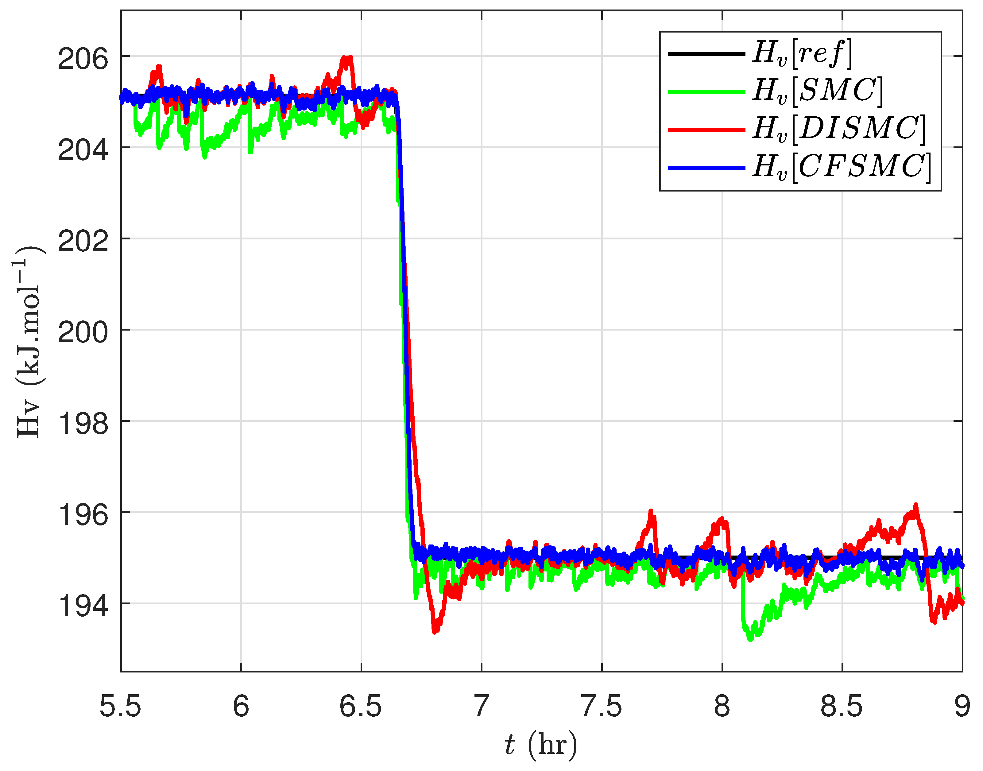
• The desired heating value trajectory is expressed in Figure 2, which represents a sudden change in the demand for electricity generation.
• The total simulation time is 9 h. To ensure that the heating value reaches the appropriate set point, the UCG system is run in an open loop for initial $5.5$ h. The flow rate of gases is maintained at $2\times {10}^{-4}$ moles $\mathrm{c}{\mathrm{m}}^{-2}{\mathrm{s}}^{-1}$ during this time. Afterward, the UCG system is run in a close loop configuration for $5.5\le t\le 9$ h. Therefore, for better visualization, the simulation results for evaluating the performance of the controllers are only shown for the closed-loop operation.
• SDKF works for the complete simulation, i.e., $0\le t\le 9$ h.
• The gains of CFSMC in (13) and (14) are: $c=69$, $\lambda =0.1$, $T=0.1$, $k_d=0.5$, $k_T=-2$, and $\eta =1$.

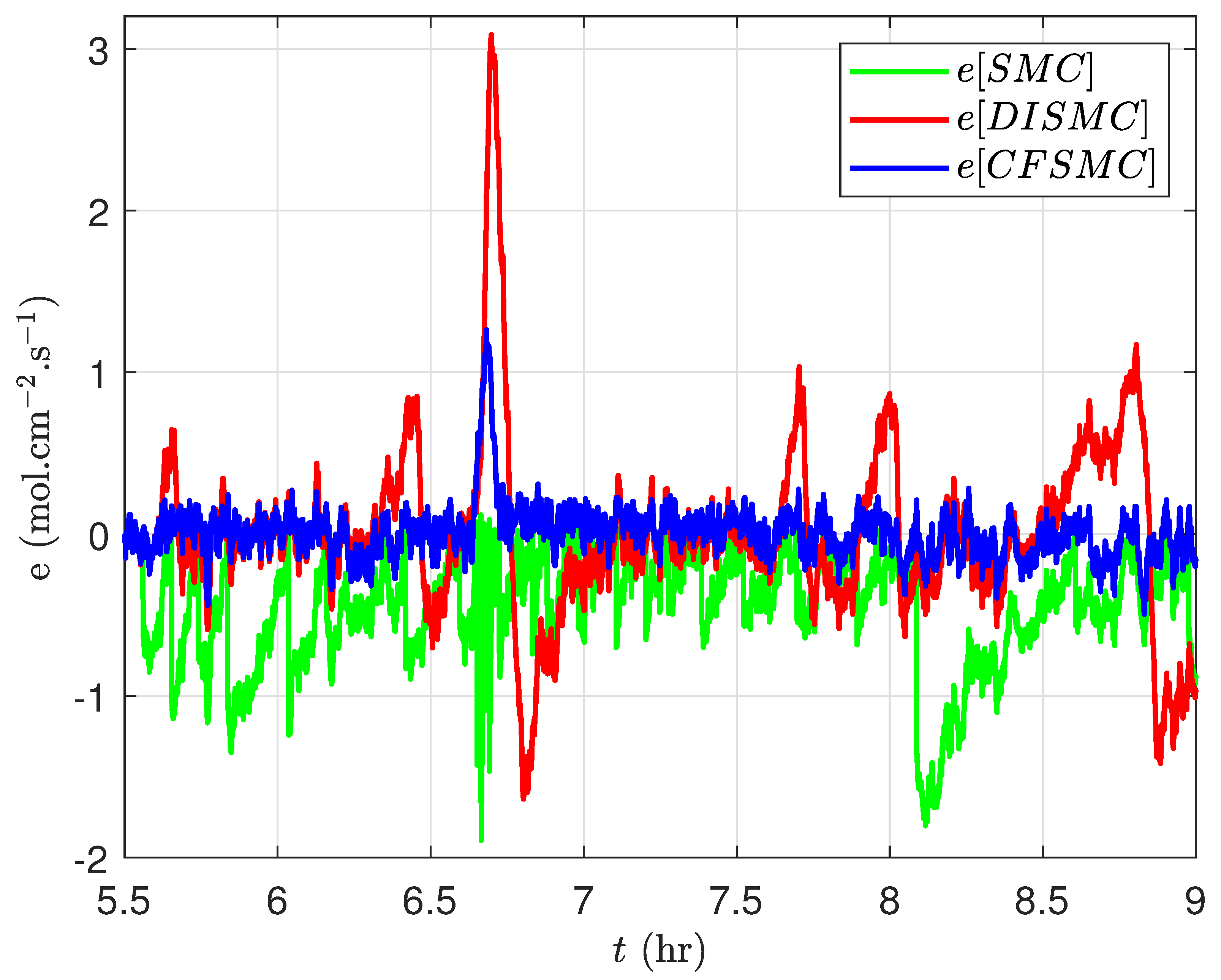
The tracking performance of the selected controllers is shown in Figure 2. The reference trajectory shows a sudden change from a higher to a lower level of the heating value. To track the abrupt change in the reference trajectory, the gains of the controllers are kept on the higher side, which results in poor performance of SMC and DISMC as compared to CFSMC. Figure 3 depicts the tracking error of different control schemes.

The manipulated flow rate of the inlet gases for different control schemes is presented in Figure 4. It is evident from the figure that the tracking performance of CFSMC is the most superior as compared to DISMC and SMC.

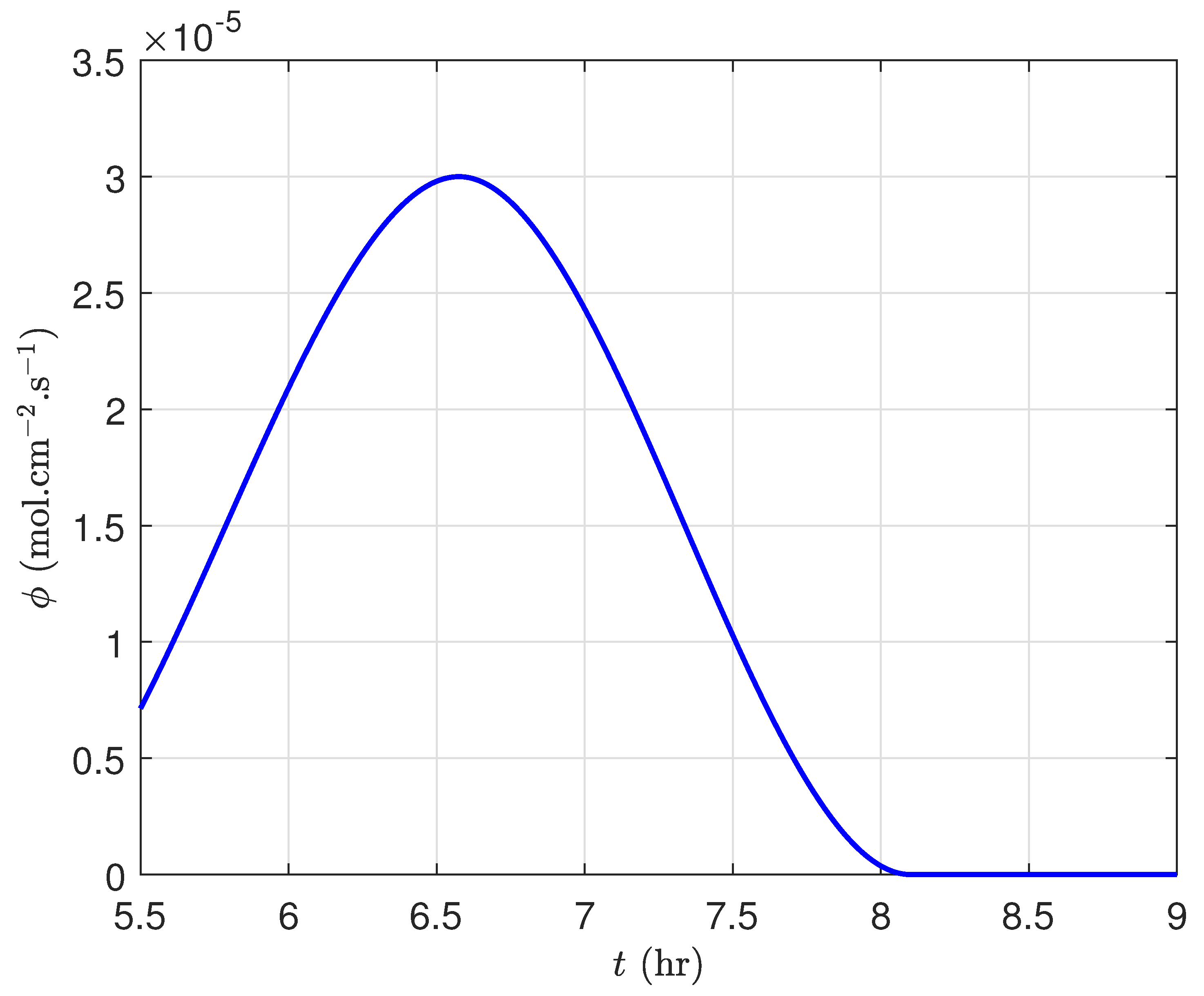
A sufficient amount of steam is necessary to ensure the smooth operation of the UCG reactor. Generally, there are two sources of steam: a mixture of the inlet gas (which in the current case contains $77\%$ steam) and water ingress from surrounding aquifers, which is considered as an external disturbance, and its time profile is depicted in Figure 5. It is evident from Figure 4 that all the controllers manipulate u to mitigate the effect of $\varphi$. However, the results in Figure 2 and Figure 3 demonstrate that CFSMC exhibits more robustness to compensate $\varphi$ as compared to DISMC and SMC.

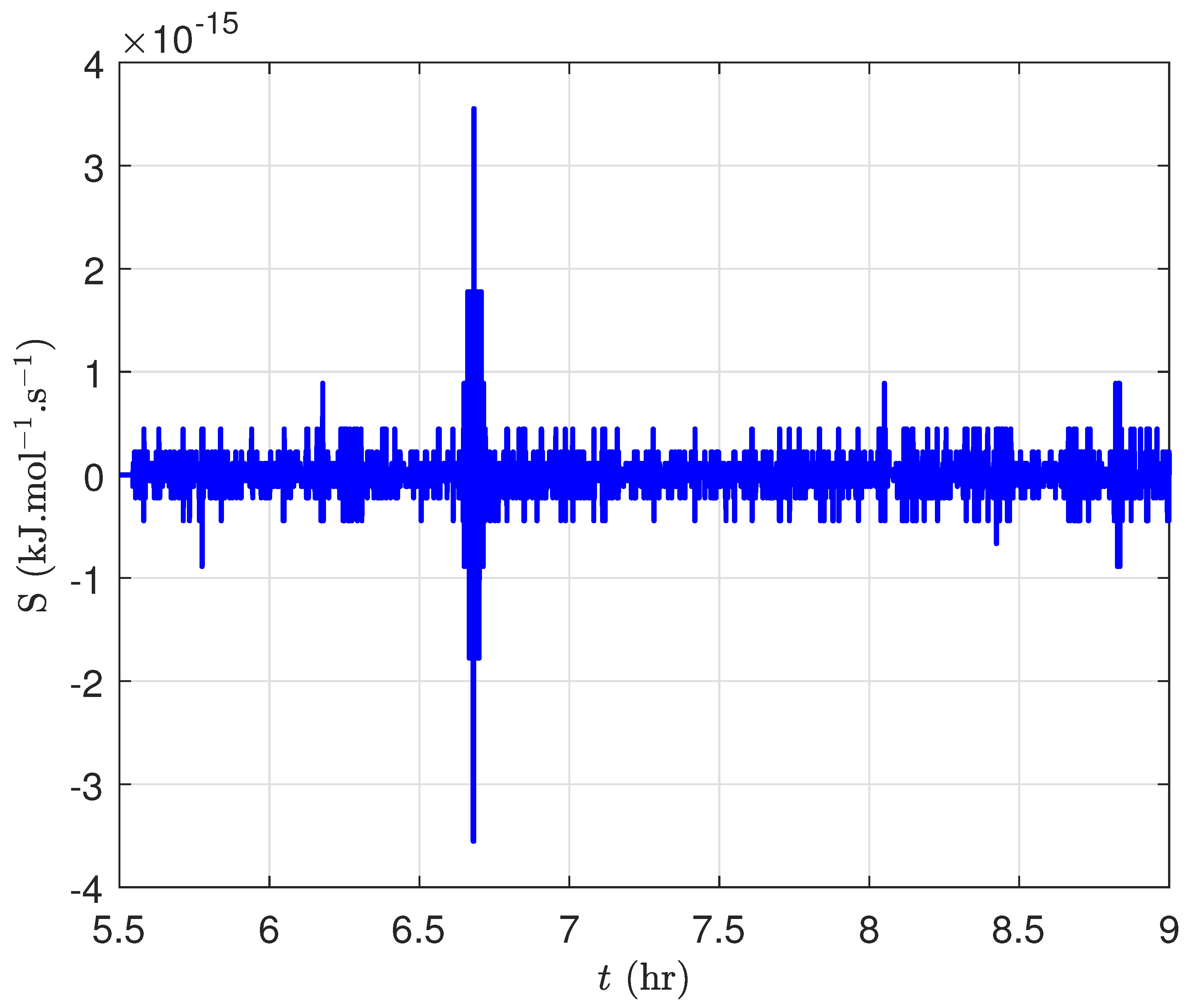
Figure 6 shows the sliding variable designed for CFSMC, which is given by (13). Despite the disturbance and measurement noise, the system trajectories are confined to the manifold $S=0$.

A comprehensive quantitative analysis has been performed to assess the performance of CFSMC, DISMC, and SMC. The attributes considered for performance evaluation are root mean squared error $e_{rms}$ and the average power $P_{avg}$ of the control input u. These performance indices are characterized as

$$\begin{array}{cc}\hfill e_{rms}& =\sqrt{{\displaystyle \frac{1}{N}}\sum _{i=1}^N{(H_v\left[i\right]-H_{vd}\left[i\right])}^2},\hfill \\ \hfill P_{avg}& ={\displaystyle \frac{1}{N}}\sum _{i=1}^N{\left(u_i\right)}^2,\hfill \end{array}$$

(32)

where N represents the number of samples.

The values of the performance indices for CFSMC, DISMC, and SMC are provided in

Table 4. Comparison of SMC, DISMC, and CFSMC.

Controller	${\mathrm{e}}_{\mathbf{rms}}$	${\mathrm{P}}_{\mathbf{avg}}$
SMC	$0.5736$	$5.0364\times {10}^{-6}$
DISMC	$0.5479$	$1.9422\times {10}^{-7}$
CFSMC	$0.1653$	$1.4981\times {10}^{-7}$

. Here, it can be seen that all the controllers consume the same control energy; however, the performance of CFSMC is superior to its counterparts. In fact, CFSMC shows $57.1\%$ and $58.9\%$ better tracking performance than SMC and DISMC, respectively.

The remaining part of the section discusses the performance of SDKF. To evaluate the estimation performance of SDKF; it is essential to start the UCG plant and GSMUO with contrasting initial conditions. The initial state vectors for the UCG process model and SDKF are selected as

$$\begin{array}{cc}\hfill x^T\left(0\right)& =\left[\begin{array}{ccccccccccc}0.5& 0& 497& 0& 0& 0& 0& 0& 0& 4.2\times {10}^{-4}& 1.6\times {10}^{-3}\end{array}\right],\hfill \\ \hfill {\widehat{x}}^T\left(0\right)& =\left[\begin{array}{ccccccccccc}0.48& 0& 480& 0& 0& 0& 0& 0& 0& 4.2\times {10}^{-4}& 1.6\times {10}^{-3}\end{array}\right].\hfill \end{array}$$

It is pertinent to mention that some values in $x\left(0\right)$ and $\widehat{x}\left(0\right)$ are equal or very close to each other; this is because the initial values of some states are known.

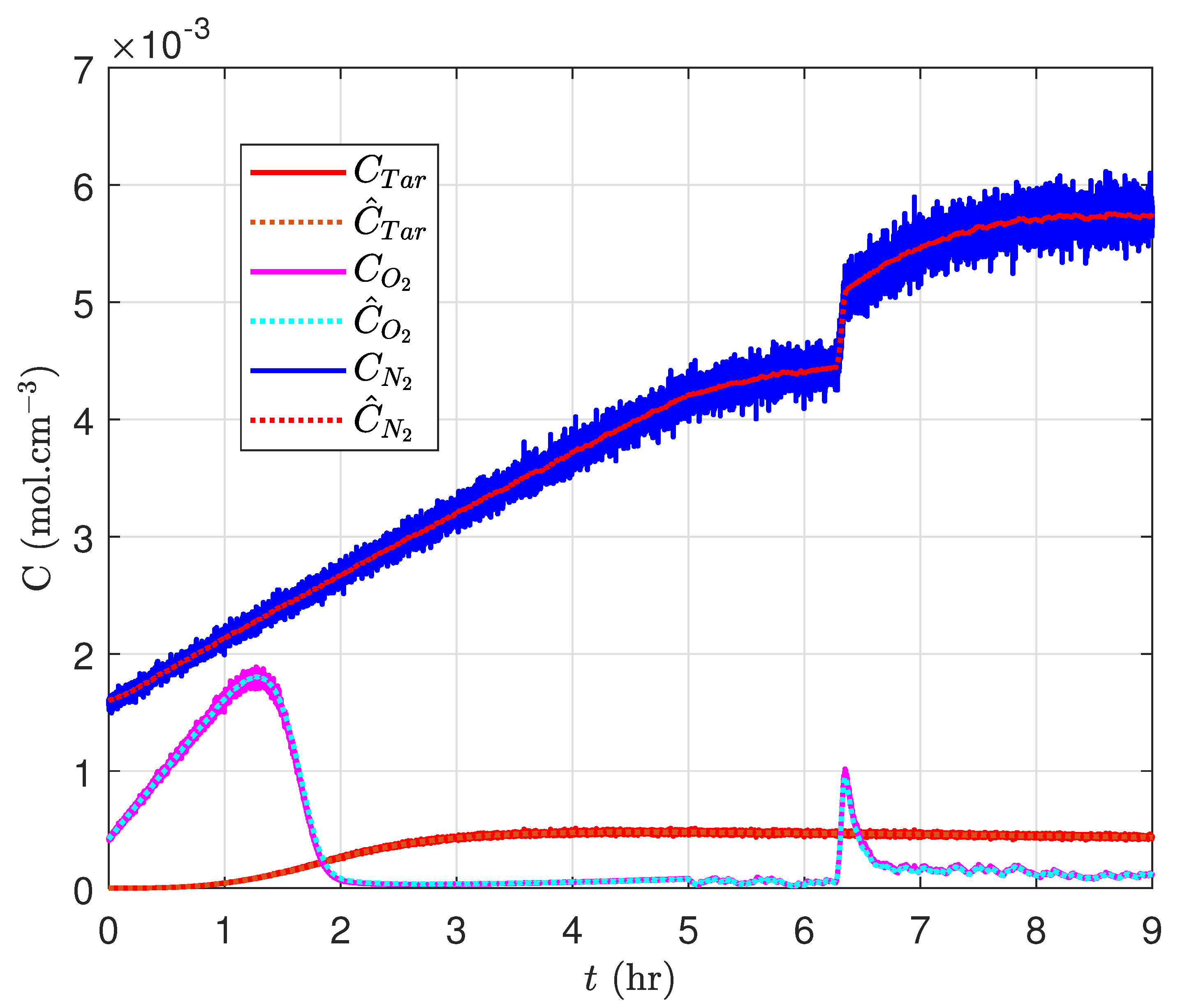
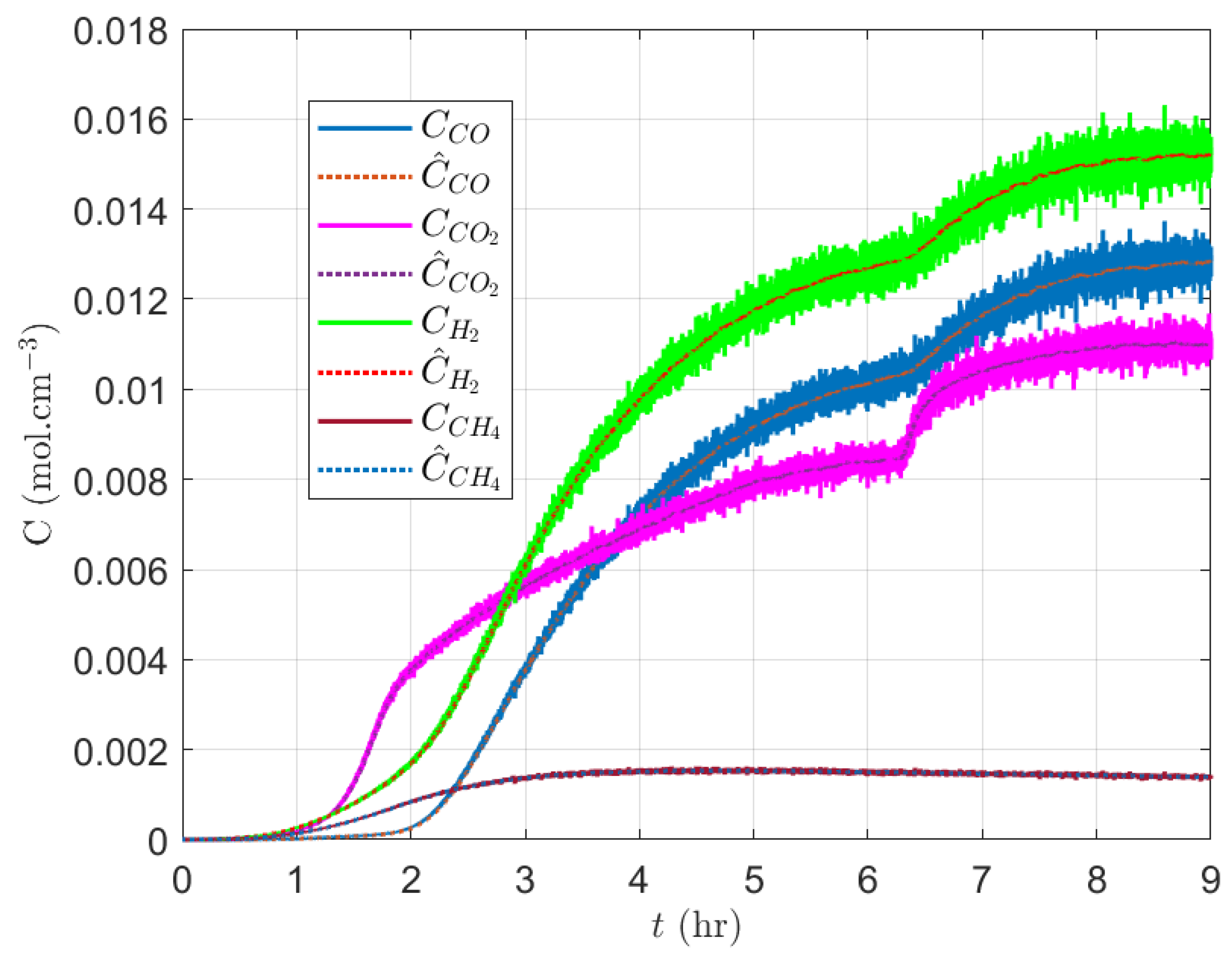
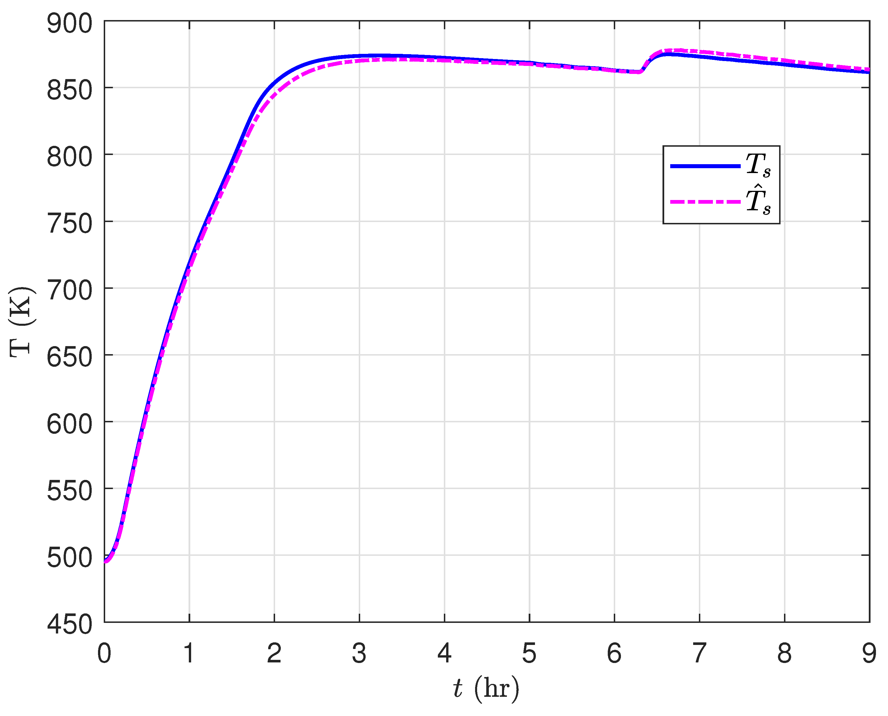
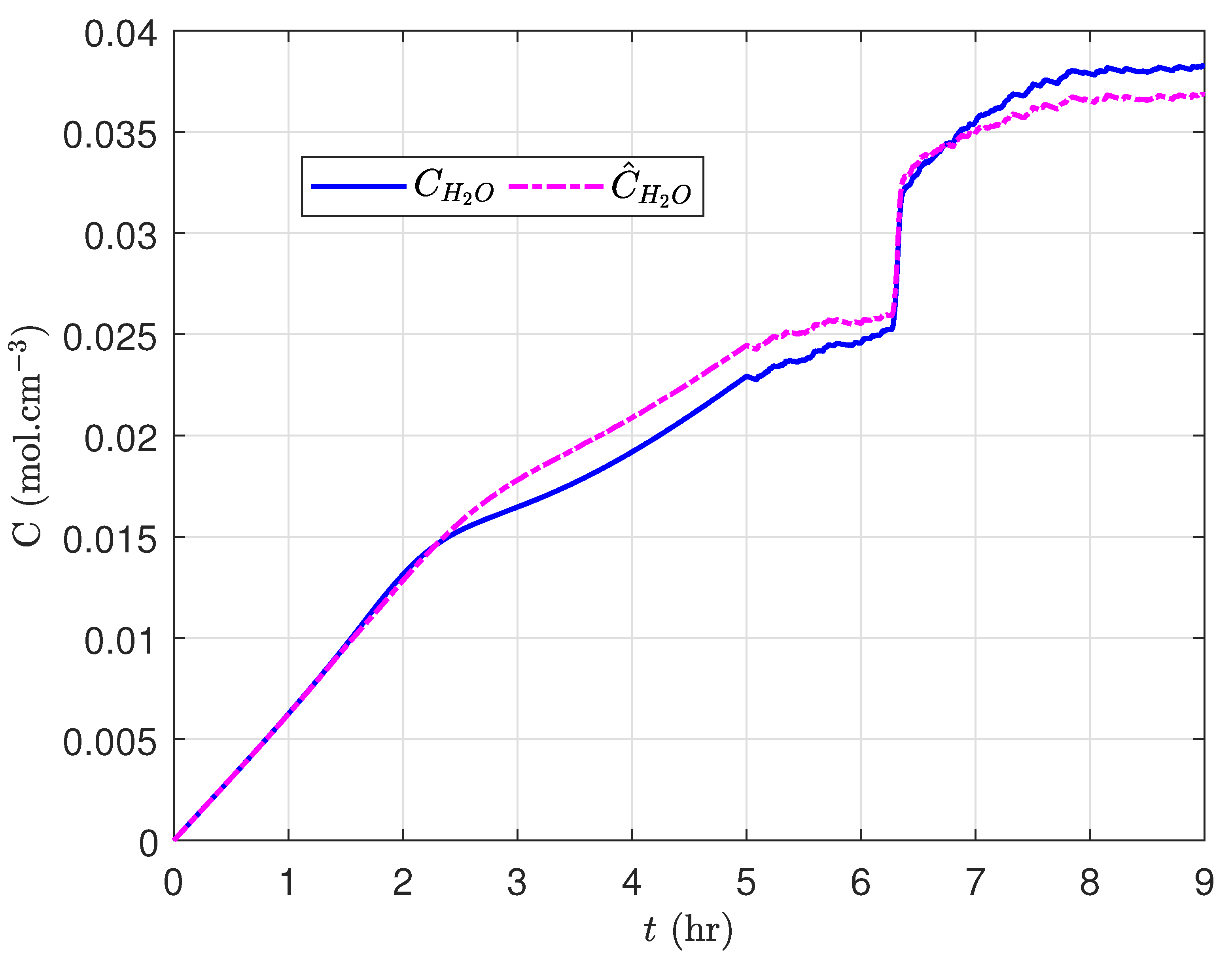
Seven out of eleven states are measurable, but a full state SDKF is designed so that the measurement noise can be filtered. The results in Figure 7 and Figure 8 demonstrate how SDKF filters out the measurement noise from the measured states. The estimated states are then used for the synthesis of the controller.

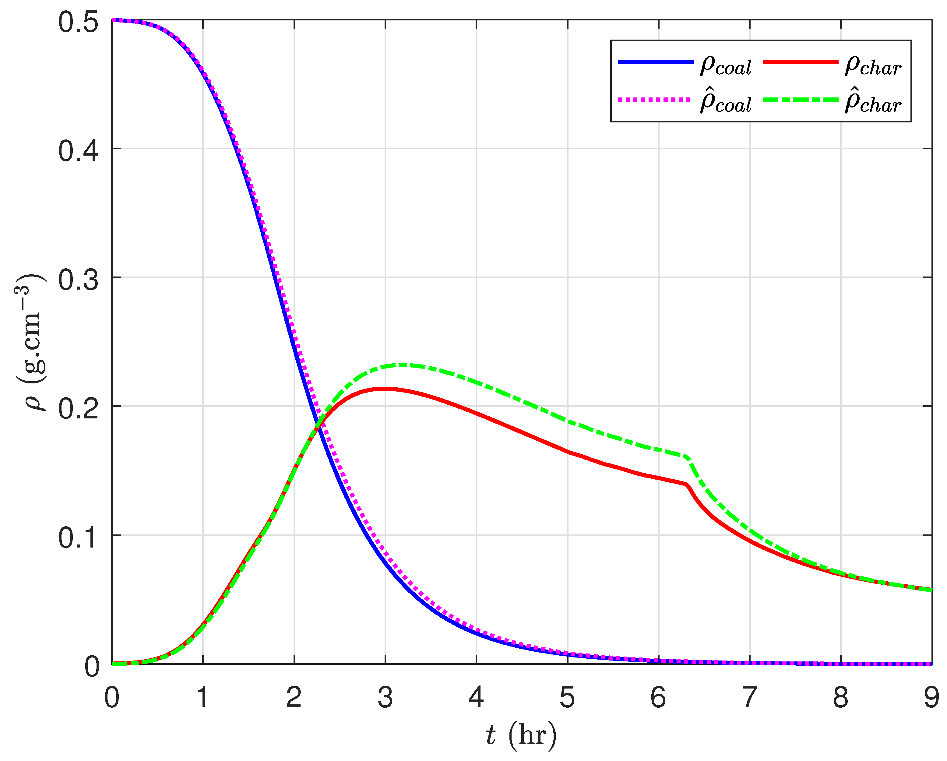
Figure 9, Figure 10 and Figure 11 depict the estimation of the unmeasurable states of the UCG model. It is evident from the simulation results that the estimated and actual states are well aligned. The difference in the true and estimated values of the steam concentration is due to the disturbance $\varphi$.

From the simulation results and comparative analysis of different control techniques, it can be seen that the performance of SDKF is slightly better than GSMUO designed in [14]. However, the design of GSMUO is quite complex as compared to SDKF, which is simply a linear discrete-time Kalman filter implemented using the quasi-linear UCG model.

6. Conclusions

In this study, a model-based CFSMC is proposed for tracking the desired heating value trajectory of the UCG process in the presence of external disturbance and measurement noise. A formal analysis of the stability of the controller is also presented. To enable the feedback control design, the unmeasurable UCG process states are estimated by utilizing SDKF, which is based on the quasi-linearization of the nonlinear UCG model. A detailed qualitative and quantitative comparison is also made between CFSMC-SDKF, SMC-SDKF, and DISMC-GSMUO techniques. The comparison demonstrates that the CFSMC-SDKF technique outperforms its counterparts for a rapidly changing reference trajectory.

A possible future extension of this work is the cascade control of the IGCC power plant, which is comprised of the UCG plant and a combined cycle turbine. The efficacy of this technique can be analyzed for tracking the sudden variations in the demand for electrical power.

References

1. Blinderman, M.; Klimenko, A. Underground Coal Gasification and Combustion; Woodhead Publishing: Sawston, UK, 2017; pp. 1–650. [Google Scholar] [CrossRef]
2. Perkins, G. Underground coal gasification—Part II: Fundamental phenomena and modeling. Prog. Energy Combust. Sci. 2018, 67, 234–274. [Google Scholar] [CrossRef]
3. Perkins, G. Underground coal gasification—Part I: Field demonstrations and process performance. Prog. Energy Combust. Sci. 2018, 67, 158–187. [Google Scholar] [CrossRef]
4. Green, M. Recent developments and current position of underground coal gasification. Proc. Inst. Mech. Eng. Part A J. Power Energy 2017, 232, 095765091771877. [Google Scholar] [CrossRef]
5. Uppal, A.A.; Bhatti, A.; Aamir, E.; Samar, R.; Khan, S. Control oriented modeling and optimization of one dimensional packed bed model of underground coal gasification. J. Process Control 2014, 24, 269–277. [Google Scholar] [CrossRef]
6. Karol, K.; Ján, K. The monitoring and control of underground coal gasification in laboratory conditions. Acta Montan. Slovaca 2008, 13, 111–117. [Google Scholar]
7. Karol, K.; Ján, K. Development of control and monitoring system of UCG by Promotic. In Proceedings of the 12th International Carpathian Control Conference (ICCC), Velke Karlovice, Czech Republic, 25–28 May 2011; pp. 215–219. [Google Scholar] [CrossRef]
8. Kačur, J.; Durdán, M.; Laciak, M.; Flegner, P. A Comparative Study of Data-Driven Modeling Methods for Soft-Sensing in Underground Coal Gasification. Acta Polytech. 2019, 59. [Google Scholar]
9. Karol, K.; Ján, K. Extremum Seeking Control of Carbon Monoxide Concentration in Underground Coal Gasification. IFAC-PapersOnLine 2017, 50, 13772–13777. [Google Scholar] [CrossRef]
10. Kacur, J.; Flegner, P.; Durdán, M.; Laciak, M. Model predictive control of UCG: An experiment and simulation study. Inf. Technol. Control 2019, 48, 557–578. [Google Scholar] [CrossRef]
11. Xiao, Y.; Yin, J.; Hu, Y.; Wang, J.; Yin, H.; Qi, H. Monitoring and control in underground coal gasification: Current research status and future perspective. Sustainability 2019, 11, 217. [Google Scholar]
12. Kačur, J.; Laciak, M.; Durdán, M.; Flegner, P. Model-free control of UCG based on continual optimization of operating variables: An experimental study. Energies 2021, 14, 4323. [Google Scholar]
13. Uppal, A.A.; Bhatti, A.I.; Samar, R.; Ahmed, Q.; Aamir, E. Model development of UCG and calorific value maintenance via sliding mode control. In Proceedings of the 2012 International Conference on Emerging Technologies, Islamabad, Pakistan, 8–9 October 2012; pp. 1–6. [Google Scholar] [CrossRef]
14. Uppal, A.A.; Butt, S.S.; Khan, Q.; Aschemann, H. Robust tracking of the heating value in an underground coal gasification process using dynamic integral sliding mode control and a gain-scheduled modified Utkin observer. J. Process Control 2019, 73, 113–122. [Google Scholar] [CrossRef]
15. YU, X.; MAN, Z. Model reference adaptive control systems with terminal sliding modes. Int. J. Control 1996, 64, 1165–1176. [Google Scholar] [CrossRef]
16. Feng, Y.; Fengling, H.; Yu, X. Chattering free full-order sliding-mode control. Automatica 2014, 50, 1310–1314. [Google Scholar] [CrossRef]
17. Yu, X.; Kaynak, O. Sliding-Mode Control With Soft Computing: A Survey. IEEE Trans. Ind. Electron. 2009, 56, 3275–3285. [Google Scholar] [CrossRef]
18. Teixeira, M.; Zak, S. Stabilizing Controller Design for Uncertain Nonlinear Systems Using Fuzzy Models. IEEE Trans. Fuzzy Syst. 1999, 7, 133–142. [Google Scholar] [CrossRef]
19. Li, Q.; Li, R.; Ji, K.; Dai, W. Kalman Filter and Its Application. In Proceedings of the 8th International Conference on Intelligent Networks and Intelligent Systems (ICINIS), Tianjin, China, 1–3 November 2015; pp. 74–77. [Google Scholar] [CrossRef]
20. Kim, Y.; Bang, H. Introduction to Kalman Filter and Its Applications; IntechOpen: London, UK, 2018; pp. 1–16. [Google Scholar] [CrossRef]
21. Chaudhry, A.M.; Uppal, A.A.; Bram, S. Model Predictive Control and Adaptive Kalman Filter Design for an Underground Coal Gasification Process. IEEE Access 2021, 9, 130737–130750. [Google Scholar] [CrossRef]
Figure 1. SDKF algorithm implementation.
Electronics 12 00876 g001
Figure 2. Syngas Heating value in the closed-loop operation with time.
Electronics 12 00876 g002
Figure 3. Tracking -error with various controllers during closed-loop operation with time.
Electronics 12 00876 g003
Figure 4. Control input for different controllers with time.
Electronics 12 00876 g004
Figure 5. Steam flow rate generated by water influx from nearby aquifers with time.
Electronics 12 00876 g005
Figure 6. Sliding manifold for CFSMC with time.
Electronics 12 00876 g006
Figure 7. Measured and estimated concentrations of gases with time.
Electronics 12 00876 g007
Figure 8. Measured and estimated concentrations of gases with time.
Electronics 12 00876 g008
Figure 9. True and reconstructed solid densities with time.
Electronics 12 00876 g009
Figure 10. True and reconstructed solid temperature with time.
Electronics 12 00876 g010
Figure 11. True and estimated steam concentration with time.
Electronics 12 00876 g011