FLRAM: Robust Aggregation Technique for Defense against Byzantine Poisoning Attacks in Federated Learning

Abstract

In response to the susceptibility of federated learning, which is based on a distributed training structure, to byzantine poisoning attacks from malicious clients, resulting in issues such as slowed or disrupted model convergence and reduced model accuracy, we propose a robust aggregation technique for defending against byzantine poisoning attacks in federated learning, known as FLRAM. First, we employ isolation forest and an improved density-based clustering algorithm to detect anomalies in the amplitudes and symbols of client local gradients, effectively filtering out gradients with large magnitude and angular deviation variations. Subsequently, we construct a credibility matrix based on the filtered subset of gradients to evaluate the trustworthiness of each local gradient. Using this credibility score, we further select gradients with higher trustworthiness. Finally, we aggregate the filtered gradients to obtain the global gradient, which is then used to update the global model. The experimental findings show that our proposed approach achieves strong defense performance without compromising FedAvg accuracy. Furthermore, it exhibits superior robustness compared to existing solutions.

1. Introduction

In recent years, with the advancement of machine learning technology, a quantum leap in computational capabilities, and the deepening of research in big data, artificial intelligence has entered its third era of research renaissance. Machine learning has not only witnessed rapid progress, but has also permeated different sectors, playing an important role. However, in order to build exceptional machine learning models, it is necessary to extract critical information from a large amount of meaningful data. This undoubtedly amplifies the complexities associated with data sharing and integration, imposing novel demands on the facets of data sharing and fusion. Simultaneously, as societies progressively emphasize individual privacy, governments worldwide intensify regulatory efforts to ensure the rightful protection of user privacy. Consequently, aversion of privacy breaches during data integration and sharing has emerged as a current focal point of research.

Federated learning [1] as an emerging distributed machine learning approach exhibits outstanding privacy protection capabilities, effectively addressing numerous issues arising from data integration. Unlike traditional machine learning, federated learning can construct a global model without the need for data to leave the local environment and subsequently distribute the constructed model to participating parties. This approach circumvents the leakage of raw data and greatly ensures the data security of each participating party [2]. However, existing research indicates that federated learning still faces certain security vulnerabilities. Attackers can exploit the distributed nature of federated learning to launch byzantine poisoning attacks [3] on local data or models involved in training. By uploading tampered local model gradients, they can contaminate the global model, not only undermining the convergence performance of the global model, but also potentially causing a significant drop in model accuracy. This byzantine poisoning attack threatens model integrity, undermines the interests of participants, and poses challenges to the overall reliability of federated learning.

To address this issue, we propose a robust aggregation technique for defending against byzantine poisoning attacks in federated learning named FLRAM. Existing robust aggregation methods in federated learning typically employ a set of strategies during the client model gradient uploading phase, such as gradient median estimation, distance detection, and clipping transformations [4], to filter out benign clients that positively influence the convergence of the global model. However, our approach differs in that it employs isolation forests and improved DBSCAN techniques for anomaly detection, specifically targeting the magnitudes and signs of the gradients uploaded by clients, to identify and exclude malicious clients that may detrimentally impact the convergence performance of the global model or affect model accuracy. Subsequently, a credibility matrix is constructed, and benign clients with higher credibility scores are selected to participate in model training. It is worth noting that whether it is model poisoning or data poisoning, both can directly or indirectly result in changes in model gradients. Therefore, if a client’s model gradient exhibits anomalies, it implies that the client is either an abnormal client or has already been subjected to a poisoning attack.

The main contributions of this paper are as follows:

• This paper proposes a federated learning robust aggregation method, FLRAM, designed to counter byzantine poisoning attacks. FLRAM employs anomaly gradient detection to filter out abnormal clients and selectively aggregates models from clients with higher credibility scores, enhancing model aggregation robustness.
• This paper introduces an improved DBSCAN algorithm for clustering gradient signs to enhance the accuracy of abnormal gradient identification. Additionally, by constructing a credibility matrix, we effectively assess the trustworthiness of each client, further bolstering the model’s robustness.
• We theoretically prove the convergence properties of the proposed method and conduct experimental validations. The experimental results demonstrate that the proposed approach not only ensures model accuracy, but also exhibits outstanding defense performance, effectively enhancing the robustness of the federated learning system.

2. Related Work

As federated learning gains widespread adoption in practical applications, its training security garners significant attention [5,6]. In federated learning, byzantine poisoning attacks refer to malicious participants tampering with model parameters or injecting harmful data to undermine the integrity and credibility of federated learning, thereby compromising its security. Given the substantial disruptive potential of byzantine poisoning attacks in federated learning, they have emerged as a focal point of current research efforts [7]. In addition, throughout this paper, subsequent references to poisoning attacks are denoted as Byzantine poisoning attacks.

In response to poisoning attacks, researchers have actively explored and proposed various defense strategies and techniques, and these defense schemes can be summarized into two broad categories: passive and active defense. Active defense aims at detecting and mitigating the risk in advance before the FL framework is affected, while passive defense aims at remediating and mitigating the impact when the attack has already occurred [8]. More specifically, the passive defense strategy usually involves the central server performing a statistical characterization of the uploaded local models after an attack has occurred and designing the appropriate aggregation method. During the aggregation process, the central server eliminates model parameters that may be subject to poisoning attacks to improve the performance of the global model [9,10,11,12,13]. For instance, Yin et al. [9] introduced the Trimmed Mean, which accomplishes model aggregation by excluding the maximum and minimum values from a specified number of model parameters and computing the mean of the remaining ones. Blanchard et al. [10] proposed Multi-Krum, which selects multiple most similar model parameters based on Euclidean distance and calculates their mean for model aggregation. Guerraoui et al. [11] presented Bulyan, which identifies and eliminates outlier clients significantly affecting the outcome by comparing the contributions of each client to the aggregation process, followed by aggregating the model parameters of the remaining clients. Luis et al. [12] proposed AFA, which calculates the weighted average of collected model parameters, computes the cosine similarity between this weighted average and the model parameters of each participant, and then combines the mean, median, and standard deviation of cosine similarities to eliminate exceptional poisoned models. Tolpegin et al. [13] extracted model parameters related to specific data labels and employed principal component analysis to reduce the dimensionality of high-dimensional model parameters. This approach is used to exclude malicious model updates and effectively aggregate normal model updates. However, in passive defense, the use of traditional statistical feature analysis may introduce potential biases, as some poisoned models may be skillfully designed to exhibit statistical features similar to those of normal models, aiming to circumvent detection by aggregation methods and thereby pollute the global model.

In contrast to passive defense, active defense methods employ proactive strategies to address poisoning attacks in federated learning in advance. Their key focus lies in the ability to detect potential malicious models promptly and exclude them to ensure the security and reliability of the global model [14,15,16,17,18]. In this approach, the performance of the local model is detected to exclude the malicious poison model, which has become a new trend of poisoning attack defense in federated learning. For instance, Bilgin et al. [14] directly calculated the similarity between model parameters of different participants, thereby assessing local model performance through the comparison of similarities and differences in local model parameters to detect potential malicious models. Liu et al. [15] proposed CoLA, which constructs a contrastive self-supervised learning task to learn model representations. They utilized the learned embeddings to compute anomaly scores for each local model. Subsequently, by analyzing these anomaly scores, they assessed model performance and eliminated exceptional models. Zhang et al. [16] introduced FLDetector, which predicts each client’s local model updates using Cauchy’s mean value theorem and the L-BFGS method. When a model update received from a client is inconsistent with the predicted local model update, it is considered an exceptional update and is removed. Zhao et al. [17] utilized generative adversarial networks to create an audit dataset on the server to evaluate the accuracy of participants’ models. If a participant’s local model accuracy falls below a preset threshold, it is considered an exceptional model. Zhu et al. [18] proposed MANDERA, which transforms local model updates from numerical gradient values to the ranking space, evaluating model performance within the ranking space. This process results in a credibility matrix that conforms to the ranking distribution. Subsequently, the method then detects clients with low credibility rankings and excludes them. However, most of the aforementioned active defense methods rely on the assumption of identically distributed data (IID) distribution. Additionally, during anomaly detection, some benign clients may be mistakenly identified as anomalies and excluded, thereby impacting the accuracy of the global model. Therefore, this paper employs effective active defense methods for detecting abnormal models and introduces reputation statistical analysis to screen participants, aiming to minimize the inadvertent exclusion of benign clients due to their characteristics or external factors. Furthermore, the proposed method is adaptable to scenarios where real-world data distributions deviate from the IID assumption, allowing for greater applicability across various settings.

3. Basic Theory

3.1. Federated Learning Aggregation Mechanism

The aggregation mechanism in federated learning is a method used to combine participant model updates and generate a global model. In federated learning, where participants protect the privacy of their local data and do not directly share model parameters, this aggregation mechanism becomes crucial for effectively integrating model updates scattered across different participants. FedAvg is the most commonly used aggregation mechanism in federated learning; however, it lacks sufficient robustness and has limited defense capabilities against external attacks. Therefore, federated learning urgently needs a robust aggregation strategy to enhance its security defenses. Below are several common gradient-based federated learning robust aggregation mechanisms.

Krum [10]: Select one gradient from the input gradient set that is closest to the squared Euclidean norm space of n-m-2 neighboring gradients as the global gradient. It can be expressed as $\overline{g}={\displaystyle \underset{g_i}{\arg \min }}{\displaystyle \sum _{g_j\in {\Omega }_{j,n-m-2}}}\left|\right|g_i-g_j{\left|\right|}_2^2$, where ${\Omega }_{j,n-m-2}$ represents a set of n-m-2 gradients closest to gradient $g_j$, n is the total number of gradients, and m is the number of malicious gradients.

Trimmed Mean [9]: Sort the values along the jth dimension of all input gradients, then remove the m largest and smallest values, and calculate the average of the remaining values as the aggregation for dimension j. The aggregated value for dimension j of the gradient is expressed as $\overline{v}=\frac{1}{n-2m}{\displaystyle \sum _{i\in U_j}}{\left(g_i\right)}_j$, where $j\in \left[d\right]$, $U_j$ represents the indices of the closest n-$2m$ values to the median, and d is the dimensionality of the gradient.

RSA [19]: Perturb all input gradients along their directions, meaning each gradient value is augmented by a perturbation equal to the sign of the difference between the gradient itself and the global gradient. It can be expressed as $g_i=g_i+\lambda sign(g_i-\overline{g})$, where $\lambda$ represents the regularization term, and then the perturbed gradients are averaged to obtain the global gradient.

FLTrust [20]: Calculate the directional similarity between all input gradients and the global gradient using cosine similarity and obtain trust scores through ReLU function clipping. It can be expressed as $TS({\mathrm{g}}_i)=ReLU\left(\frac{〈{\mathrm{g}}_i,{\mathrm{g}}_0〉}{\left|\right|{\mathrm{g}}_i\left|\right|·\left|\right|{\mathrm{g}}_0\left|\right|}\right)$. Subsequently, normalize each local gradient to maintain a certain magnitude relative to the global gradient. Finally, employ trust scores to weigh and aggregate the normalized local gradients to obtain the global gradient. It can be expressed as $\overline{g}=\frac{1}{{\sum }_{i=1}^{n}TS\left(g_i\right)}{\sum }_{i=1}^{n}TS\left(g_i\right)·\frac{\left|\right|g_0\left|\right|}{\left|\right|g_i\left|\right|}{g}_i$, where $g_0$ denotes the global gradient from the previous iteration.

3.2. Isolated Forest

Isolated Forest (iForest) is an unsupervised learning technique for detecting anomalies [21]. Its central concept is to analyze the degree of isolation of samples in the feature space in order to establish their anomalous status. Specifically, it employs a binary tree structure to isolate samples. Given that anomalous samples often exhibit sparse distributions and are distant from regions of higher data density, this enables the swift identification and isolation of anomalous samples within the tree structure.

The process of anomaly detection using Isolated Forest consists of two phases. The first phase is the training phase, where we construct a forest composed of t isolation trees. Initially, a random sample of $\phi$ data points from the given dataset $X=x_1,x_2,\dots ,x_n$ is placed at the root node. Then, a random dimension is chosen, and a splitting point p is randomly generated within the current data range, such that min<p<max, where min and max represent the minimum and maximum values in the current data. Subsequently, the current data space is divided into two subspaces using the splitting point p. Data points with values less than p in the specified dimension are placed in the left subspace, while those greater than or equal to p are placed in the right subspace. This process is repeated recursively until $\left|X\right|=1$ or the height of the isolation tree reaches a predefined limit, at which point a single isolation tree is fully constructed. This entire process is iterated until a total of t isolation trees are successfully constructed.

The second phase, known as the prediction phase, involves iterating over each data point $x_i$. For each data point, we traverse each isolation tree in the Isolated Forest. We calculate the average path length $E\left[h\left(x_i\right)\right]$ of the data point within the Isolated Forest. Subsequently, we normalize the average path lengths of all points and compute the anomaly score for each point using the following formula:

$$s(x,\phi )=2^{-\frac{E\left[h\right(x\left)\right]}{c\left(\phi \right)},}$$

(1)

where

$$c\left(\phi \right)=2H(\phi -1)-2(\phi -1)/\phi ,$$

(2)

$H\left(\phi \right)=ln\left(\phi \right)+\zeta$, where $\zeta$ is the Euler constant. Regarding anomaly scores, the higher their values, the more likely a data point is to be isolated. Therefore, data points with higher anomaly scores are considered anomalies, completing the anomaly detection process using the Isolated Forest.

3.3. DBSCAN

DBSCAN is an unsupervised density-based clustering algorithm [22] capable of discovering clusters of arbitrary shapes in feature spaces that may contain noisy samples. This algorithm employs parameters $(\epsilon ,MinPts)$ to characterize the distribution of samples within neighborhoods, where $\epsilon$ represents the neighborhood radius and MinPts denotes the threshold for the number of samples in the neighborhood of a given sample, which are at a distance of $\epsilon$ or less. For any sample point $x_j\in D$ (where D is the sample set), if its neighborhood $N_{\epsilon }\left(x_j\right)=dis(x_i,x_j)\le \epsilon$ ($x_i\in D$) contains at least MinPts samples, then $x_j$ is considered a core point. Here, $dis\left({\displaystyle \blacksquare }\right)$ represents the Euclidean distance. If $x_j$ is not a core point but lies within the neighborhood of some core point, it is classified as a border point. Any point that is neither a core point nor a border point is regarded as a noise point.

The distance relationships between data points can be categorized as density-reachable, density-reachable, density-connected, and non-density-connected. If a sample point $x_i$ is within the $\epsilon$-neighborhood of $x_j$, and $x_j$ is a core object, then $x_i$ is said to be density-reachable from $x_j$. If there exists a sequence of sample points $x_i,x_{i+1},\dots ,x_{j-1},x_j$ such that $x_{i+1}$ is density-reachable from $x_i$, …, and $x_j$ is density-reachable from $x_{j-1}$, then $x_j$ is considered density-reachable from $x_i$. If there exists a core sample point $x_k$ such that both $x_i$ and $x_j$ are density-reachable from $x_k$, then $x_i$ and $x_j$ are considered density-connected. If sample points $x_i$ and $x_j$ do not share a density-connected relationship, they are termed non-density-connected.

4. Problem Description

4.1. Problem Definition

The federated learning system consists of a centssral server and K clients, where each client possesses a local training dataset $D_i,i=1,2,\dots ,K$. $D={\bigcup }_{i=1}^K{D}_i$ represents the data involved in the training. The collective objective of all clients is to collaboratively train a shared global model $w^{*}$ under the coordination of the central server. The optimal global model is denoted as

$$w^{*}=\underset{w}{argmin}\{F(w,D)\triangleq \frac{1}{K}\sum _{i=1}^{K}F(w_i,D_i)\}.$$

(3)

Each client conducts local training to address the following optimization problem:

$$\underset{w_i}{min}F(w_i,D_i)=\underset{w_i}{min}\frac{1}{|D_i|}\sum _{j=1}^{|D_i|}\xi (w_i,D_i),$$

(4)

where $|D_i|$ denotes the training data quantity for client i, and $\xi \left({\displaystyle \blacksquare }\right)$ represents the loss function. After completing local training, clients send their local gradients to the central server, considering the presence of a certain number of anomalous (malicious) clients who may send arbitrary gradient information $g_m$ to the central server. Therefore, the local gradient can be expressed as

$$g_i=\left\{\begin{array}{c}\nabla F_i\begin{array}{cc}(w;D)& \mathrm{Benign}\mathrm{client}\end{array}\hfill \\ g_m\begin{array}{cc}& \begin{array}{cccc}& & & \end{array}\mathrm{Malicious}\mathrm{client}\end{array}\hfill \end{array}\right.,$$

(5)

where $\nabla F_i(w;D)$ represents the local gradient sent by normal (benign) clients. Subsequently, the server aggregates the collected gradient information to obtain the global gradient, which is then utilized to update the global model.

$$w_{t+1}=w_t-{\eta }_{t}GAR\left\{g_{i,t}\right\},$$

(6)

where ${\eta }_t$ represents the learning rate for the tth iteration, GAR stands for the Gradient-based aggregation rules. The objective of the paper is to formulate an appropriate GAR to defend against poisoning attacks by malicious clients.

4.2. Attack Model

During the training process in federated learning, malicious clients can tamper with local model parameters or inject malicious samples into local data to corrupt model parameters. These malicious clients can exert control over other clients and compromise the models and data within the clients. They can freely send their local gradients to the central server and selectively participate in each round of global gradient update iterations. These malicious clients may collaborate to undermine the integrity of the model. However, it is assumed that the number of malicious clients, denoted as C, does not exceed half of the total number of clients participating in training, i.e., $C<K/2$. These malicious clients may or may not be aware of the aggregation rules employed by the central server; those who know the aggregation rules are considered strong adversaries, while others are considered weak adversaries.

4.3. Defensive Target

In federated learning, to effectively defend against poisoning attacks, robust aggregation methods should fulfill the following key objectives:

(1)

Fidelity: Ensure that the accuracy of the globally aggregated model after aggregation remains close to the accuracy of the model obtained through FedAvg in the absence of attacks.

(2)

Robustness: The globally aggregated model should maintain a high level of accuracy even when multiple malicious clients engage in poisoning attacks simultaneously, or when certain malicious clients conduct strong poisoning attacks.

(3)

Reliability: The defense performance against different datasets and various poisoning attacks should exhibit stability. The aggregation method should apply to a general attack model and not be susceptible to a specific type of attack that causes a rapid deterioration in model performance.

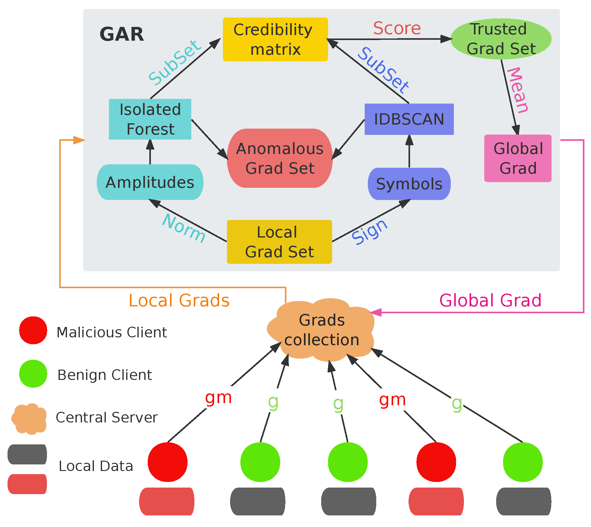
5. FLRAM Frame

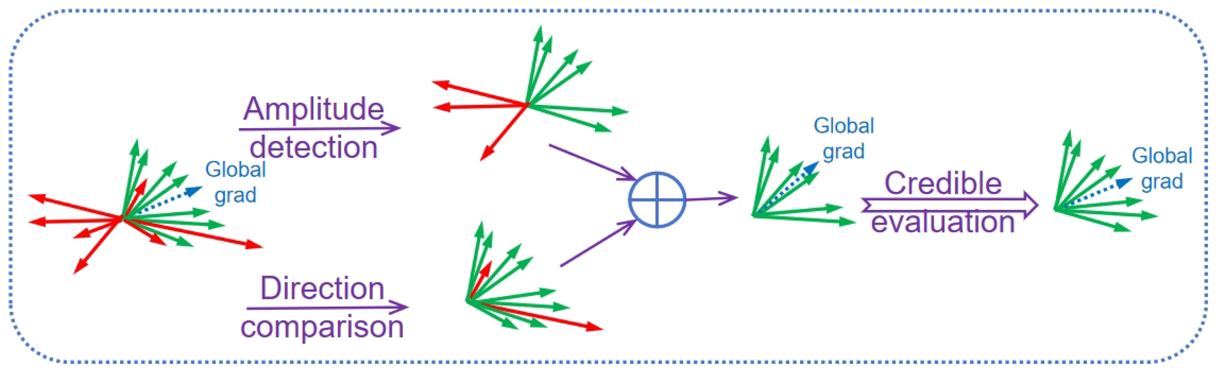
5.1. Method Overview

To effectively defend against poisoning attacks during the federated learning training process, this paper proposes a federated learning robust aggregation method for defense, as illustrated in Figure 1. Here, $g_m$ represents the gradients uploaded by malicious clients, and g denotes the gradients uploaded by benign clients. After collecting local gradients, the central server employs an isolation forest for anomaly detection based on gradient amplitudes and employs an enhanced DBSCAN algorithm for clustering based on gradient symbols to filter out anomalous gradient sets. Subsequently, a credibility matrix is constructed based on this subset of gradients, and trusted gradient sets are further selected based on their credibility scores. Finally, these filtered gradient sets are simply averaged to form the global gradient.

5.2. Method Design

FLRAM is primarily divided into three major components, aiming to achieve robust defense aggregation against poisoning attacks in federated learning. These three core stages are Anomalous Gradient Detection, Credibility Assessment, and Global Gradient Aggregation. Each of these is introduced in detail below.

5.2.1. Anomaly Gradient Detection

During the training process in federated learning, some malicious clients may employ various interference techniques to disrupt the model training. These interference methods include adding random noise to their uploaded local gradients (distinct from the noise addition in differential privacy, which aims to prevent the leakage of specific individual data in global model training), or altering the direction of gradient signs. The gradients with added noise significantly differ numerically from normal gradients, which can slow down the convergence speed of the model. In addition, reversing the gradient signs leads to the model training deviating from its regular convergence path, potentially causing training to fail to achieve the expected convergence results.

To prevent malicious clients from affecting the training results by modifying gradient amplitudes, some current defense strategies [23,24] employ gradient clipping to correct the gradient amplitudes and reduce the interference of malicious gradients with the global gradient. However, clipped gradients may not fully convey the updated information from benign clients, diminishing their contribution to model aggregation and potentially slowing down model convergence. Therefore, rather than modifying amplitudes, this paper uses the isolation forest algorithm for anomaly detection on gradient amplitudes, identifying and removing anomalous gradients to reduce their impact on the global gradient. The steps are as follows:

(1)

Compute the norm of the local gradient uploaded by each client, then input it into the isolation forest model. Calculate the anomaly score for each local gradient norm based on the average path length of the trees as follows:

$$S_i=2^{-\frac{E\left[h\right(\left|\right|g_i{\left|\right|}_2^2\left)\right]}{c\left(\phi \right)}},$$

(7)

where $c\left(\phi \right)$ can be obtained from Equation (2). The range of $S_i$ is (0,1), where $S_i$ approaching one indicates a higher degree of gradient anomaly, and $S_i$ approaching zero indicates a lower degree of gradient anomaly.

(2)

Calculate the dynamic anomaly score threshold $\gamma$. Compute the anomaly scores for all local gradients, and then use the percentile rank of sorted anomaly score values as the anomaly score threshold. It can be expressed as

$$\gamma =\left\{\begin{array}{cc}{S}_{⌊\frac{C(K+1)}{K}⌋+1}\hfill & \frac{C(K+1)}{K}\notin Z\hfill \\ \frac{1}{2}(S_{⌊\frac{C(K+1)}{K}⌋}+S_{⌊\frac{C(K+1)}{K}⌋+1})\hfill & \frac{C(K+1)}{K}\in Z\hfill \end{array}\right.,$$

(8)

where C represents the estimated number of anomalous clients, and K denotes the total number of clients. Under the assumptions we made, the valid range for C is in the interval $\left[1,\frac{K}{2}\right)$. At the outset of model training, we collect all local gradients and initialize the value of C to $\frac{K}{2}$. Subsequently, during the training process, the value of C is dynamically adjusted to ensure the effective identification of gradients with significant size deviations by the isolation forest detection.

(3)

Determine the degree of anomaly for each gradient based on the anomaly score threshold $\gamma$. When $S_i\le \gamma$, the gradient is labeled as normal, and when $S_i>\gamma$, label it as an anomalous gradient. Subsequently, collect all the benign gradients and store them in a candidate subset ${\Omega }_1$.

Due to the effectiveness of gradient amplitude anomaly detection in addressing variations in gradient numerical values, when certain outlier clients perturb only a portion of the signs of their local gradients while ensuring that the magnitude of the gradients remains unchanged, relying solely on anomaly detection of gradient magnitudes may not yield satisfactory results. As a result, clustering methods are used to detect abnormalities in gradient signs in order to alleviate the issue of gradient angle deviation produced by malevolent clients’ partial sign perturbations. In the current literature, researchers often use variants of DBSCAN for clustering local gradients. By selecting high-density cluster centers, they aim to eliminate gradients with significantly deviated angles. For instance, in reference [25], HDBSCAN is used to cluster local gradients, with only the MinPts threshold set. Although this approach effectively aggregates most benign gradients, the classification results for boundary gradients may not be stable. HDBSCAN employs a hierarchical clustering strategy to determine the cluster structure, tending to form core regions with high density and consider boundary gradients as part of the cluster. This may result in the ambiguity of boundary gradients and the exclusion of some of them as anomalous gradients. In reference [26], AdaptDBSCAN is used for clustering, with the median of cosine distances between gradients as the neighborhood radius $\epsilon$ and $⌊\frac{n}{2}⌋$ as the MinPts threshold. While this method dynamically adjusts cluster centers and assigns gradients to the most suitable clusters, some strong adversarial clients can control the cosine distances between their local gradients and other gradients to fall within an appropriate range. For instance, in Min–Max attacks [27], they continuously adjust the distances between gradients, ensuring that the maximum distance between an anomalous gradient and any other gradient is smaller than the maximum distance between any two benign gradients (including cosine distances). Under such attacks, although cluster centers can be dynamically changed, they utilize global distances to measure $\epsilon$, making them somewhat vulnerable. This paper employs an improved version of DBSCAN—IDBSCAN to perform local measurements of $\epsilon$, making $\epsilon$ vary from one gradient object to another. It utilizes similarity to assess whether a gradient object’s $\epsilon$ is a core object, i.e., whether the number of similar gradient objects (within its neighborhood) exceeds MinPts. This allows for a more precise characterization of gradient signs during clustering. Specifically, the sign function is initially used to count the number of positive and negative signs in each local gradient, represented as

$$SF\left(g_i\right)=\left\{\begin{array}{c}\sum _{j=1}^d\left[sign\left({\left(g_i\right)}_j\right)\right][{\left(g_i\right)}_j>0],{\left(g_i\right)}_j>0\hfill \\ \sum _{j=1}^d[sign\left({\left(g_i\right)}_j\right)=0][{\left(g_i\right)}_j=0],{\left(g_i\right)}_j=0\hfill \\ \sum _{j=1}^d\left[sign\left({\left(g_i\right)}_j\right)\right][{\left(g_i\right)}_j<0],{\left(g_i\right)}_j<0\hfill \end{array}\right.,$$

(9)

where d represents the dimensionality of gradients, $SF\left(g\right)$ is a statistical tuple. Considering that perturbations to some signs of the gradients can lead to changes in the statistics of positive, negative, and zero values in the uploaded gradients, i.e., certain component signs may be perturbed, switching from positive to negative or zero or vice versa, such perturbations can result in alterations in the statistics mentioned in Equation (9). These ternary statistical tuples, i.e., positive, negative, and zero counts, can be used as features input into the IDBSCAN for clustering and subsequent anomaly detection. The clustering process in IDBSCAN is as follows:

(1)

For each gradient sign feature $x_i=SF\left(g_i\right)$, obtain the k-nearest neighbors using the k-nearest neighbor algorithm to form a set:

$$knn(x_i,k)=\left\{x_j\right|dis(x_i,x_j)\le dis(x_i,x_k),j=1,2,..,k\}.$$

(10)

Calculate $\epsilon$ locally based on the k-nearest neighbors of each gradient sign feature $knn\left(x_i\right)$, setting it equal to the maximum distance to the k neighbors,

$$\epsilon =max\{dis(x_i,x_j),j=1,2,\dots ,k\},$$

(11)

where $dis\left({\displaystyle \blacksquare }\right)$ represents the Euclidean distance.

(2)

Calculate the density similarity between every two adjacent gradient symbol features (the ratio of the local densities of two gradient symbol features). Define the local density of each gradient symbol feature $x_i$ as the sum of lengths to its MinPts nearest neighbors as follows:

$$ld\left(x_i\right)=\sum _{j=1}^{MinPts}dis(x_i,x_j).$$

(12)

Calculate density similarity based on local density

$$ds(x_i,x_j)=\left\{\begin{array}{c}\frac{ld\left(x_i\right)}{ld\left(x_j\right)}\begin{array}{cc}& ld\left(x_i\right)\le ld\left(x_j\right)\end{array}\\ \frac{ld\left(x_j\right)}{ld\left(x_i\right)}\begin{array}{cc}& ld\left(x_i\right)>ld\left(x_j\right)\end{array}\end{array}\right..$$

(13)

(3)

Calculate the number of similar neighbors to the gradient symbol feature $x_i$ (count the number of density similarities greater than the similarity threshold):

$$sn\left(x_i\right)=\sum _{j=1}^k[ds(x_i,x_j)-{\gamma }_{ds}],$$

(14)

where ${\gamma }_{ds}$ is the similarity threshold, which, in this paper, is taken as the mean of all density similarities of gradient symbol features.

The Pseudocode of IDBSCAN can be seen in Algorithm 1:

Algorithm 1 IDBSCAN

Input:  X local gradient sign feature set; $MinPts$ a threshold value; k the number of neighbors; Output:  ${\Omega }_2$ density-based cluster set; 1: Mark all gradient objects in the local gradient sign feature set X as ‘unvisited’; 2: for $x_i\in X$ do 3:     Compute the K-nearest neighbor set $knn(x_i,k)$, along with the corresponding neighborhood radius $\epsilon$; 4:     Calculate the local density $ld\left(x_i\right)$; 5:     Calculate the density similarity $ds(x_i,x_j)$ for all gradient objects within the $\epsilon$ neighborhood of $x_i$; 6: end for 7: Compute the similarity threshold ${\gamma }_{ds}\leftarrow Mean\left(ds\left(X\right)\right)$; 8: for $x_i\in X$ do 9:     Mark $x_i$ as visited and calculate the number of similar neighbors $sn\left(x_i\right)$; 10:     for $x_j\in N_{\epsilon }\left(x_i\right)$ do 11:         if $x_j$ is unvisited then 12:            Add objects from $N_{\epsilon }\left(x_j\right)$ that do not belong to any cluster to C 13:            if $sn\left(x_j\right)\ge MinPts$ then 14:                Add objects from $N_{\epsilon }\left(x_j\right)$ that are not assigned to any cluster to C 15:            end if 16:            ${\Omega }_2\leftarrow C$ // Assign the cluster set to ${\Omega }_2$ 17:         else 18:            $x_i$ is a noise point; 19:         end if 20:     end for 21: end for 22: Output ${\Omega }_2$;

5.2.2. Credit Evaluation

After the filtering process with isolation forest and IDBSCAN, we obtain local gradients that are closer to the global gradient in both amplitude and sign. However, aggregating the global gradient solely using these filtered gradient subsets may still lead to the inclusion of certain anomalous gradients, affecting the convergence of the global model. While taking the intersection of these two filtered subsets can maximize the filtering of benign gradients and ensure alignment with the normal convergence direction, real-world scenarios can be more complex. For instance, some clients may predominantly send normal gradients but occasionally transmit anomalous ones due to malicious activities, and they should not be excluded for extended periods. Moreover, as the training rounds progress, more experienced attackers may employ increasingly covert and disruptive attack strategies, resulting in the persistence of anomalous gradients in the filtering process. At the same time, some otherwise benign clients may be misjudged because the gradient in a particular situation is similar to the abnormal gradient.

To address the aforementioned issues, we construct a trustworthiness matrix based on the filtered gradient subsets, which allows us assessment of the credibility of each local gradient. Through credibility scoring, we can further filter out the more trustworthy gradients. The steps for evaluating the credibility of local gradients and obtaining the set of benign gradients are as follows:

(1)

Labeling Gradients as Normal/Anomalous. We collect the filtered candidate gradient subsets ${\Omega }_1$ and ${\Omega }_2$ after anomaly gradient detection. Then, we introduce instance labels $y_s$ and assign a label of 1 to the gradients selected in the intersection, while gradients not included in either gradient subset ${\Omega }_1$ or ${\Omega }_2$ are labeled as −1, and all other gradients are labeled as 0. It is represented as

$$y_s=\left\{\begin{array}{cc}\hfill 1& {\Omega }_1\cap {\Omega }_2\\ \hfill -1& 1-{\Omega }_1\cup {\Omega }_2\\ \hfill 0& other\end{array}\right..$$

(15)

(2)

Building the credibility matrix. At the initial stage of model training, we initialize a matrix consisting of all-zero elements, with the indices corresponding to the gradients from different clients. In this matrix, the first row holds counting values $cv$. During each iteration, if a gradient is labeled as normal, represented as 1, the counting value for the respective client increases by 1. If the gradient is labeled as abnormal, denoted as −1, the corresponding counting value decreases by 1. Another row in the matrix records the credibility of gradients, denoted as $cw$. It represents the average frequency with which a gradient is selected and participates in training. The calculation formula for $cw$ is $cw=cv/E$, where E represents the number of iterations.

(3)

Compute Credibility Scores. We adjust the credibility $cw$ using a sigmoid function to constrain the values between [−1, 1], expressed as

$$s\left(g_i\right)=\frac{1}{1+e^{-cw}}.$$

(16)

(4)

Selecting the Set of Benign Gradients. Given that the number of malicious clients is less than half of the total clients, the TopK algorithm can be employed to select the top 50% of clients based on their credibility scores. This helps reduce the risk of benign clients being excluded due to misclassification.

5.2.3. Aggregation Strategy

Aggregation of the higher-credibility benign gradients is performed using a simple average to obtain the global gradient, which is then distributed to each client for the next iteration. The global gradient after aggregation for round t is represented as follows:

$${\widehat{g}}_t=\sum _{i=1}^{\tau }\frac{1}{\tau }{g}_{i,t},$$

(17)

where $\tau$ represents the number of filtered credible gradients. The acquisition of the global gradient is illustrated in Figure 2.

The Pseudocode of FLRAM can be seen in Algorithm 2:

Algorithm 2 FLRAM

Input:  G local gradient set; t the number of isolation trees; $\phi$ the subsampling size; $\tau$ the count of trusted gradients after filtering; Output:  $\widehat{g}$ global gradient; 1: Initialize gradient subsets ${\Omega }_1={\Omega }_2=⌀$; 2: $iForest\left(iTree\right(G),t,\phi )$ // Generate t isolation trees; 3: Calculate the anomaly score $S_i$ for each local gradient $g_i$; 4: Calculate the dynamic anomaly score threshold $\gamma$; 5: ${\Omega }_1\leftarrow G\left\{i\left|sign\right(S_i-\gamma )<0\right\}$ //Collect all benign gradients; 6: Calculate the dynamic anomaly score threshold $\gamma$; 7: $X\leftarrow SF\left(G\right)$ //Collect all gradient sign features; 8: ${\Omega }_2\leftarrow \mathrm{I}DBSCAN\left(X\right)$ //Cluster the sign features using IDBSCAN; 9: Calculate the credibility $cw\leftarrow count({\Omega }_1,{\Omega }_2)$; 10: Calculate the credibility score $s\leftarrow sigmoid\left(cw\right)$; 11: $I_{good}\leftarrow G\left\{id|id=Topk(s,\tau )\right\}$ //Select local gradients with higher credibility scores; 12: Calculate the global gradient $\widehat{g}\leftarrow Mean\left(I_{good}\right)$; 13: Output $\widehat{g}$;

5.3. Convergence Analysis

In this section, we delve into the convergence analysis of FLRAM. The global model obtained through robust aggregation methods can be represented as follows:

$$w_{t+1}=w_t-{\eta }_t\nabla F\left({\omega }_t\right),$$

(18)

where $\nabla F\left({\omega }_t\right)$ represents the global gradient. Inspired by the convergence analysis of distributed optimization in [28,29], we assume that (18) satisfies the following properties:

Proposition 1

(Lipschitz condition [30]). If the objective function $F(·)$ is L-Lipschitz, then, for $\forall x,y$, it satisfies $\left|\right|F\left(x\right)-\nabla F\left(x\right)\left|\right|\le L\left|\right|x-y\left|\right|$, where $\nabla F(·)$ represents the gradient function, and $\left|\right|·\left|\right|$ denotes the norm.

Proposition 2

(L-Smoothness [31]). if the objective function $F(·)$ is L-Smooth, for $\forall x,y$, it satisfies $F\left(y\right)-F\left(x\right)\le 〈\nabla F\left(x\right),(y-x)〉+\frac{L}{2}\left|\right|y-x|{|}^2$, where $〈{\displaystyle \blacksquare }〉$ denotes the inner product of vectors.

Proposition 3

(Unbiasedness [32]). For each client i with local data, the local stochastic gradient $g_i\triangleq \nabla F(x;D_i)$ is unbiased. It can be expressed as $E\left[g_i\right]=\nabla F_i\left(x\right)$.

Proposition 4

(Boundedness [33]). For each client i, there exists a constant σ such that the local random gradient has a uniformly bounded variance. It can be expressed as $E\left[\right||g_i-\nabla F_i\left(x\right)\left|{|}^2\right]\le {\sigma }^2$. Furthermore, there exists a constant σ such that the local gradient deviates from the global gradient as $\left|\right|\nabla F_i\left(x\right)-\nabla F\left(x\right)|{|}^2\le {\delta }^2$.

We consider global aggregation in the presence of $(1-\beta )K$ malicious clients uploading malicious gradients. After detecting these malicious gradients, the expected aggregation result is the average of $\beta K$ benign gradients, which deviates from the global gradient in the absence of an attack. This bias is described by the following lemma:

Lemma 1.

Under the assumed conditions, the deviation between the average gradients of $\beta K$ clients, denoted as ${\widehat{g}}_i$, and the true global gradient $\nabla F\left(w\right)$ can be characterized as follows: $E\left[\right||\widehat{g}-\nabla F\left(w\right)\left|{|}^2\right]\le {\delta }^2+\frac{{\sigma }^2}{\beta K}$. The detailed proof can be found below.

Proof of Lemma 1.

For any arbitrary subset ${\Omega }_1$ taken from all clients, with $|{\Omega }_1|=\beta K$, where $0.5\le \beta \le 1$, we let $X=\sum _{i\in \Omega }[g_i-\nabla F\left(w{t}^{}\right)]$. According to the properties assumed and Jensen’s inequality, we can obtain

$$\left|\right|E\left[X\right]|{|}^2\le \beta \mathrm{K}\sum _{i\in \Omega }\left|\right|\nabla F_i\left(w_t^{}\right)-\nabla F\left(w_t^{}\right)|{|}^2\le {\beta }^2{\mathrm{K}}^2{\delta }^2.$$

(19)

Utilizing the properties of variance, we can derive

$$E\left|\right|X|{|}^2=\left|\right|E\left[X\right]|{|}^2+var\left[X\right]\le {\beta }^2{\mathrm{K}}^2{\delta }^2+\beta K{\sigma }^2.$$

(20)

Furthermore, we can obtain

$$E\left[\right||\widehat{g}-\nabla F\left(w_t^{}\right)|{|}^2]=E[\left|\right|\frac{1}{|\Omega |}\sum _{i\in \Omega }{g}_i-\nabla F\left(w_t^{}\right)|{|}^2]=\frac{1}{{\beta }^2{K}^2}E\left|\right|X|{|}^2\le {\delta }^2+\frac{{\sigma }^2}{\beta K},$$

(21)

which completes the proof. □

Combining the properties and lemma stated above, the convergence of FLRAM is characterized through the following theorem:

Theorem 1.

Assuming that FLRAM adopts a learning rate of ${\eta }_t\le 1/\alpha \mathrm{L}$, its convergence can be characterized as follows: $\frac{1}{T}{\displaystyle \sum _{t=0}^T}E\left[\right||\nabla F\left(w_t^{}\right)|{|}^2]\le \frac{F\left(w_0^{}\right)-F^{*}}{{\eta }_{t}T}+{\eta }_t{\Delta }_1-{\Delta }_2$, where the constant $F^{*}=minF\left(\omega \right)$, ${\Delta }_1=\frac{{\delta }^{2}L}{2}+\frac{{\sigma }^{2}L}{2\beta K}$, and ${\Delta }_2=\alpha {\delta }^2/2;+\alpha {\sigma }^2/2\beta K$, where $\alpha >0$, β is set to 0.5 in this paper, and T represents the number of iterations. The detailed proof can be found below.

Proof of Theorem 1.

Based on the assumptions of Proposition 2 and Proposition 3, we can derive

$$E\left[F\left(w_{t+1}^{}\right)\right]\le F\left(w_t^{}\right)+\langle \nabla F\left(w_t^{}\right),E[w_{t+1}^{}-w_t^{}]\rangle +\frac{L}{2}E\left[\right||w_{t+1}^{}-w_t^{}{\left|\right|}_{}^2].$$

(22)

We split the original expression, where one part is

$$\begin{array}{cc}\hfill \langle \nabla F\left(w_t^{}\right),E[w_{t+1}^{}-w_t^{}]\rangle & \le -{\eta }_t〈\nabla F\left(w_t^{}\right),E\left[{\widehat{g}}_t\right]〉=-{\eta }_t〈\nabla F\left(w_t^{}\right),E[{\widehat{g}}_t-\nabla F\left(w_t^{}\right)+\nabla F\left(w_t^{}\right)]〉\hfill \\ \hfill & \le -{\eta }_t〈\nabla F\left(w_t^{}\right),E[{\widehat{g}}_t-\nabla F\left(w_t^{}\right)]〉-{\eta }_t\left|\right|\nabla F\left(w_t^{}\right)|{|}^2\hfill \end{array}.$$

(23)

According to vector properties and the Young’s inequality, we can obtain

$$\begin{array}{cc}\hfill 〈\nabla F\left(w_t^{}\right),E[{\widehat{g}}_t-\nabla F\left(w_t^{}\right)]〉& \le \left|\right|\nabla F\left(w_t^{}\right)\left|\right|·E\left|\right|[{\widehat{g}}_t-\nabla F\left(w_t^{}\right)]\left|\right|\hfill \\ \hfill & \le \frac{1}{2\alpha }\left|\right|\nabla F\left(w_t^{}\right)|{|}^2+\frac{\alpha }{2}E\left|\right|[{\widehat{g}}_t-\nabla F\left(w_t^{}\right)]|{|}^2\hfill \\ \hfill & \le \frac{1}{2\alpha }\left|\right|\nabla F\left(w_t^{}\right)|{|}^2+\frac{\alpha {\delta }^2}{2}+\frac{\alpha {\sigma }^2}{2\beta K}.\hfill \end{array}$$

(24)

The other part of the original expression, based on Lemma 1 and Jensen’s inequality, can be obtained as follows:

$$\begin{array}{cc}\hfill E\left[\right||w_{t+1}^{}-w_t^{}|{|}_{}^2]& ={\eta }_t^{2}E\left[\right||{\widehat{g}}_t{\left|\right|}_{}^2]={\eta }_t^{2}E\left[\right||{\widehat{g}}_t-\nabla F\left(w_t^{}\right)+\nabla F\left(w_t^{}\right){\left|\right|}_{}^2]\hfill \\ \hfill & \le {\eta }_t^{2}E\left[\right||{\widehat{g}}_t-\nabla F\left(w_t^{}\right)|{|}^2]+{\eta }_t^2\left|\right|\nabla F\left(w_t^{}\right)|{|}^2\hfill \\ \hfill & \le {\eta }_t^2{\delta }^2+{\eta }_t^2\frac{{\sigma }^2}{\beta K}+{\eta }_t^2\left|\right|\nabla F\left(w_t^{}\right)|{|}^2.\hfill \end{array}$$

(25)

Integrating (22) and (24), we can obtain

$$\begin{array}{cc}\hfill E\left[F\left(w_{t+1}^{}\right)\right]& \le F\left(w_t^{}\right)-{\eta }_t\left|\right|\nabla F\left(w_t^{}\right)|{|}^2-{\eta }_t(\frac{1}{2\alpha }\left|\right|\nabla F\left(w_t^{}\right)|{|}^2+\frac{\alpha {\delta }^2}{2}+\frac{\alpha {\sigma }^2}{2\beta K})\hfill \\ \hfill & +\frac{L}{2}({\eta }_t^2{\delta }^2+{\eta }_t^2\frac{{\sigma }^2}{\beta K}+{\eta }_t^2\left|\right|\nabla F\left(w_t^{}\right)\left|{|}^2\right)\hfill \end{array},$$

(26)

where $\delta$ and $\sigma$ are constant terms, both greater than zero. Rearranging, we have

$$\begin{array}{cc}\hfill {\eta }_t(1+\frac{1}{2\alpha }-\frac{L}{2}{\eta }_t)E\left[\right||\nabla F(w_t^{})\left|{|}^2\right]& \le E[F(w_t^{})-F(w_{t+1}^{})]\hfill \\ \hfill & -(\frac{\alpha {\delta }^2{\eta }_t}{2}+\frac{\alpha {\sigma }^2{\eta }_t}{2\beta K})+(\frac{{\eta }_t^2{\delta }^{2}L}{2}+\frac{{\sigma }^2{\eta }_t^{2}L}{2\beta K})\hfill \end{array}.$$

(27)

When ${\eta }_t\le 1/\alpha L$, we obtain $1+1/2\alpha -{\eta }_t;L/2;\ge 1$. Substituting this, we can further derive

$$\frac{1}{T}\sum _{t=0}^{T}E\left[\right||\nabla F(w_t^{})|{|}^2]\le \frac{F(w_0^{})-F^{*}}{{\eta }_{t}T}+{\eta }_t(\underset{{\Delta }_1}{\underbrace{\frac{{\delta }^{2}L}{2}+\frac{{\sigma }^{2}L}{2\beta K}}})-(\underset{{\Delta }_2}{\underbrace{\frac{\alpha {\delta }^2}{2}+\frac{\alpha {\sigma }^2}{2\beta K}}}),$$

(28)

which completes the proof. □

6. Experimental Evaluation

6.1. Experimental Setup

The experimental platform used in this study runs on a 64-bit Windows 11 operating system. The development environment was PyCharm, and the programming language employed was Python 3.9. In terms of hardware configuration, the experiment was conducted on a system with an Intel(R) Core(TM) (Santa Clara, CA, USA) i7-12650H CPU, 16 GB of RAM, a 512 GB solid-state drive, and an NVIDIA GeForce RTX 3060 GPU with 6 GB of VRAM. PyTorch 1.12.1 was used to train the deep learning model. The datasets selected for the experiments included the MNIST handwritten digit dataset, comprising 60,000 training samples and 10,000 test samples. Additionally, the CIFAR-10 color image dataset was used, consisting of 50,000 training samples and 10,000 test samples.

6.1.1. Baseline and Parameter Settings

In this subsection, the baseline method chosen for comparison was the defenseless FedAvg method. It was compared with FLRAM, which is equipped with defense capabilities, as well as other methods proposed by Blanchard et al. [10] proposing Krum, Yin et al. [9] proposing Trimmed Mean (TrMean), Li et al. [19] proposing RSA, Cao et al. [20] proposing FLTrust, Shejwalkar et al. [27] proposing Dnc, and Nguyen et al. [25] proposing FLAME. To validate the effectiveness of FLRAM, a series of experiments were conducted on the MNIST and CIFAR-10 datasets. Convolutional Neural Networks (CNNs) were used as the neural network models in the experiments, with a common structure consisting of three convolutional layers and three fully connected layers. After each convolutional layer, a pooling layer and a Dropout layer were added. The model optimization algorithm used during training was Stochastic Gradient Descent (SGD) with an initial learning rate of 0.05 and a momentum factor of 0.9. Learning rate decay was implemented using an exponential decay strategy, and the batch size for training was set to 128. In the context of federated learning, 50 clients participated in the training process, with each client performing 2 local training iterations. The global training consisted of 100 iterations. Independently distributed data were primarily used for training to validate the method’s effectiveness. Additionally, the impact of Non-independent identically distributed (Non-IID) real-world data on the experiments was evaluated.

6.1.2. Attack Mode

The experiments involve comparing several typical poisoning attacks, including Sign-Flip attacks, the Mix attack [34], the Fang attack [35], the Byz attack [36], the LIE attack [37], and the Min–Max attack [27]. For the Sign-Flip Attack, malicious clients first train genuine model parameter gradients locally and then flip the signs of the gradients, represented as $g_i\leftarrow -g_i$, before sending them to the central server. In the Mix Attack, malicious clients are divided into two groups: one group adds random Gaussian noise to the gradients, and the other group scales the gradients to varying degrees before submitting them to the central server. As for the Fang Attack, it employs a carefully designed adaptive partial knowledge attack strategy, which means that the attackers do not fully understand the aggregation rules. For Krum and TrMean, the Fang Attack uses the attack strategy from reference [35]. For other aggregation methods, in the Fang Attack, malicious client i observes the global gradient to determine the local gradient transformation direction $s_j$. When $s_j=-1$, it randomly samples C values from interval [${\mu }_j+3{\sigma }_j$, ${\mu }_j+4{\sigma }_j$] as the jth parameter of the malicious client gradient. When $s_j=1$, it randomly samples C values from interval [${\mu }_j-4{\sigma }_j$, ${\mu }_j-3{\sigma }_j$], where ${\mu }_j$ and ${\sigma }_j$ represent the mean and standard deviation of the jth parameter of the malicious gradient. In the Byz Attack, malicious clients randomly sample C gradients from a standard normal distribution with mean zero and unit standard deviation and send them to the central server. In the LIE Attack, assuming that malicious clients estimate the mean $g_{mean}$ and standard deviation $g_{std}$ of all client gradients based on empirical knowledge, they replace their local gradients with $g_i\leftarrow g_{mean}+z_{max}{g}_{std}$, where $z_{max}$ is determined based on the cumulative standard normal function $\phi \left(z\right)$ as described in reference [37]. The LIE Attack primarily seeks a range in which the gradients can deviate from the mean without detection, achieved by making small changes to the gradient magnitude. However, altering the sign of the gradient in the LIE Attack requires a larger $z_{max}$. In the Min–Max Attack, malicious clients continuously search for the optimal scaling factor $\gamma$ based on empirical knowledge and replace their local gradients with $g_i\leftarrow g_{mean}-\gamma g_{std}$. In this context, the perturbation method involves reversing the standard deviation, i.e., $g_{std}=-std\left({\mathrm{g}}_i\right|i\in \left[K\right])$. The optimization of $\gamma$ is described in reference [27]. The Min–Max Attack adjusts $\gamma$ continuously, ensuring that the malicious gradient’s maximum distance from any other gradient is smaller than the maximum distance between any two benign gradients. LIE and Min–Max Attacks are more covert and have stronger disruptive potential compared to other attacks.

6.1.3. Evaluation Metrics

To assess the defensive performance of FLRAM, this paper evaluates defense schemes based on the model test accuracy.

6.2. Experimental Results and Analysis

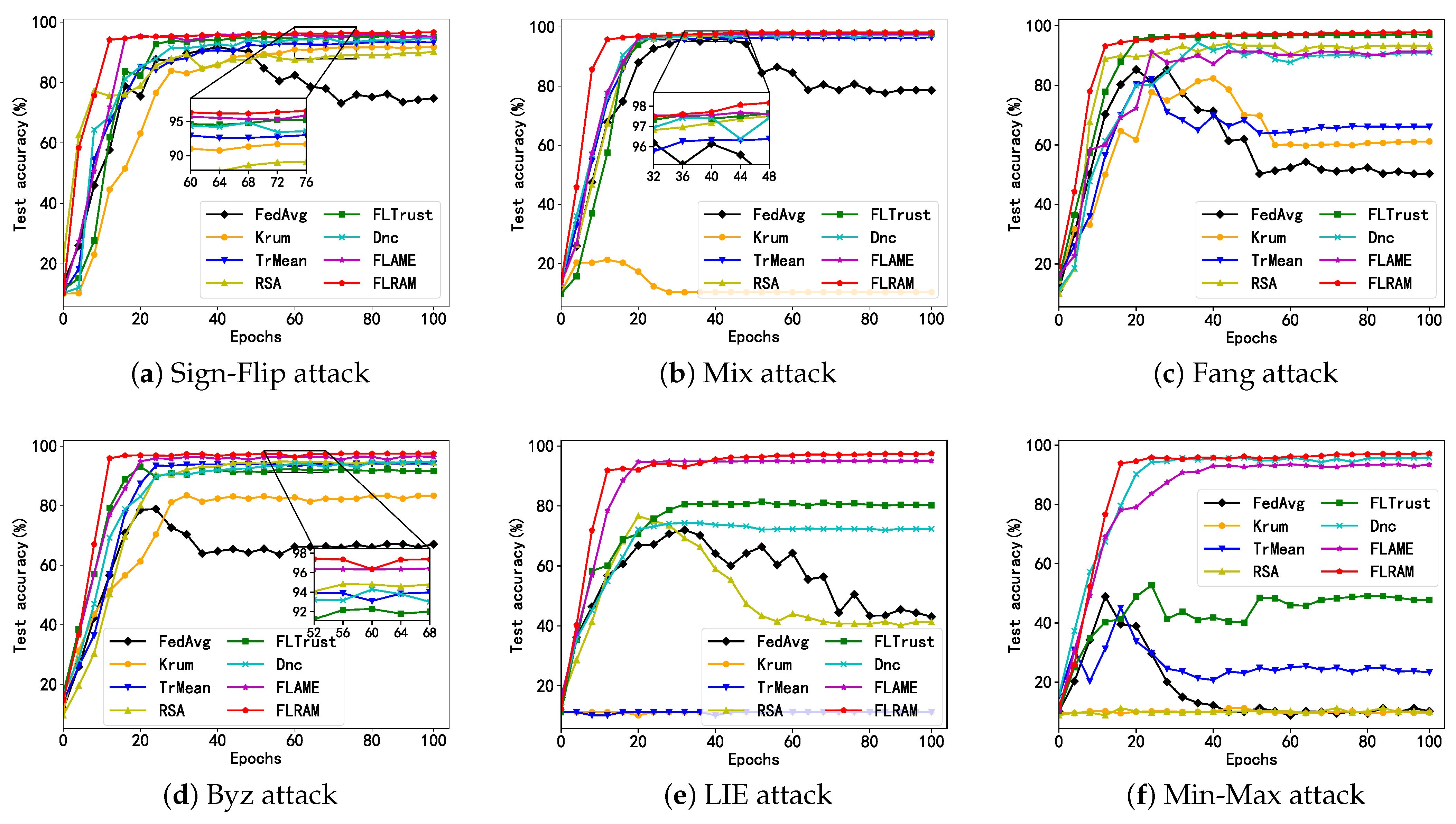
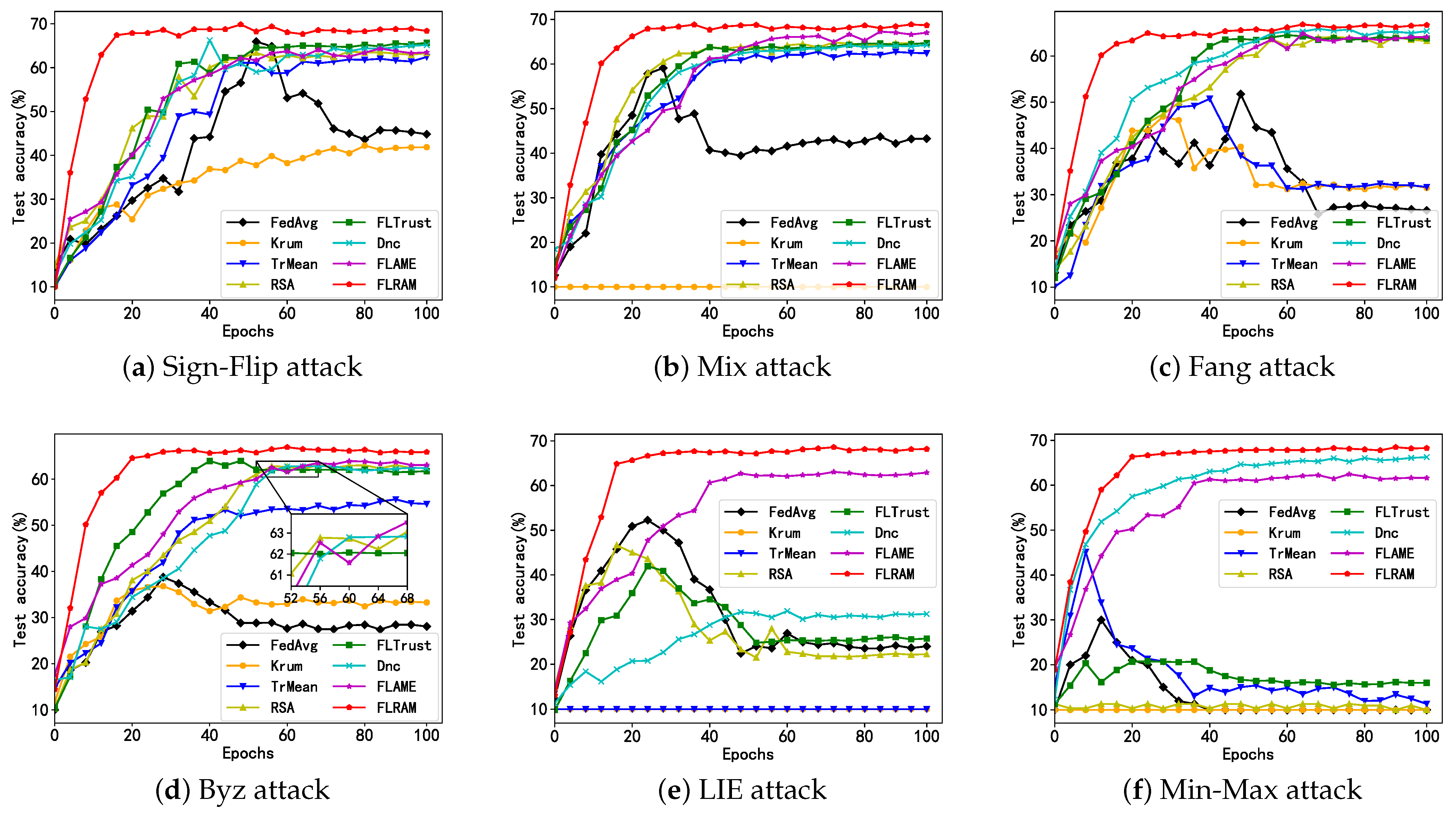
6.2.1. Comparison of Defensive Performance among Different Aggregation Methods

To validate the fidelity of FLRAM, comparisons were conducted with other aggregation methods on the MNIST and CIFAR10 datasets, assessing model accuracy in the absence of attacks. For different attack strategies, experiments selected 10 out of 50 clients as malicious clients to evaluate the methods’ resistance to attacks. The experimental results on the MNIST and CIFAR10 datasets are shown in

Table 1. Test accuracy of various aggregation methods under the MNIST dataset.

Aggregation	FedAvg	Krum	TrMean	RSA	FLTrust	Dnc	FLAME	FLRAM
No-Attack	99.01	95.15	98.48	98.92	98.38	98.89	98.79	98.94
Sign-Flip	97.28	91.88	98.06	97.64	98.23	98.31	98.21	98.53
Mix	96.37	89.16	97.94	97.61	98.19	98.35	98.01	98.43
Fang	85.35	84.92	85.58	95.02	94.79	96.67	97.95	98.40
Byz	79.21	87.71	95.86	95.62	92.51	96.41	97.47	98.39
LIE	74.28	56.35	73.94	74.12	81.31	75.69	95.75	98.05
Min-Max	49.72	41.37	55.36	* 1	55.15	97.41	93.42	97.82

¹ Indicating failure to converge properly.

and

Table 2. Test accuracy of various aggregation methods under the CIFAR10 dataset.

Aggregation	FedAvg	Krum	TrMean	RSA	FLTrust	Dnc	FLAME	FLRAM
No-Attack	75.92	52.05	69.63	73.08	73.55	74.87	69.53	73.75
Sign-Flip	69.80	48.70	66.17	67.88	69.85	70.58	68.58	71.75
Mix	69.65	51.98	68.78	67.52	69.05	69.79	68.47	70.92
Fang	61.20	47.58	59.02	65.83	66.03	68.49	67.18	70.67
Byz	57.13	51.25	67.18	66.68	64.72	68.05	67.76	70.31
LIE	52.08	23.54	47.21	53.44	58.72	45.66	66.78	69.62
Min-Max	26.23	* 1	21.79	* 1	25.69	67.89	63.73	69.22

¹ Indicating failure to converge properly.

. From the tables, it can be observed that in the absence of attacks, FLRAM achieves test accuracy on different datasets that are comparable to that of FedAvg without defense, demonstrating FLRAM’s excellent fidelity.

Meanwhile, when not subjected to attacks, Krum test accuracy showed a certain decline. This may be because Krum primarily selects a specific client based on distance when choosing clients to participate in training, ignoring the influence of other clients on the global model, resulting in a decrease in global accuracy. In the face of various poisoning attacks, FLRAM consistently demonstrated robust performance. On the MNIST dataset, against symbol flip attacks, Mix attacks, Fang attacks, Byz attacks, LIE attacks, and Min–Max attacks, FLRAM accuracy decreased by 0.41%, 0.51%, 0.54%, 0.55%, 0.89%, and 1.12%, respectively, compared to the no-attack scenario. On the CIFAR10 dataset, these decreases were 1.00%, 1.83%, 2.08%, 1.44%, 3.13%, and 3.53%, respectively. Considering the characteristics of the dataset itself and its impact on the neural network model, the accuracy of the CIFAR10 dataset is relatively lower. However, overall, FLRAM exhibited minimal differences in model accuracy in the face of various attacks. Particularly when facing more covert and destructive attacks, FLRAM defense performance remained robust. The reason for FLRAM’s high defense performance lies in the following aspects: As observed from Figure 2, by using abnormal gradient detection in combination with credibility estimation, FLRAM can effectively eliminate abnormal gradients to a maximum extent. Subsequently, the model updates, excluding abnormal gradients, are aggregated, resulting in predicted global gradients that closely approximate the actual global gradients. Therefore, FLRAM effectively ensures model accuracy.

When facing different attack strategies, it is evident that the defensive capabilities of certain aggregation methods are put to the test. From Table 1 and Table 2, it can be clearly seen that on different datasets, when the RSA method is used to defend against Min–Max attacks, the model training may fail to converge. This situation primarily arises because RSA was originally designed to introduce perturbations related to the gradient direction, preventing specific types of attacks such as direction reversal. However, the impact of Min–Max attacks has a relatively low correlation with gradient direction, resulting in a significant reduction in RSA defensive effectiveness in this scenario. Similarly, using the Krum method to counter Min–Max attacks is also not very effective. Krum relies mainly on distances between gradients for defense, but Min–Max attacks carefully control the distances between malicious clients and others, greatly undermining the effectiveness of Krum’s defense.

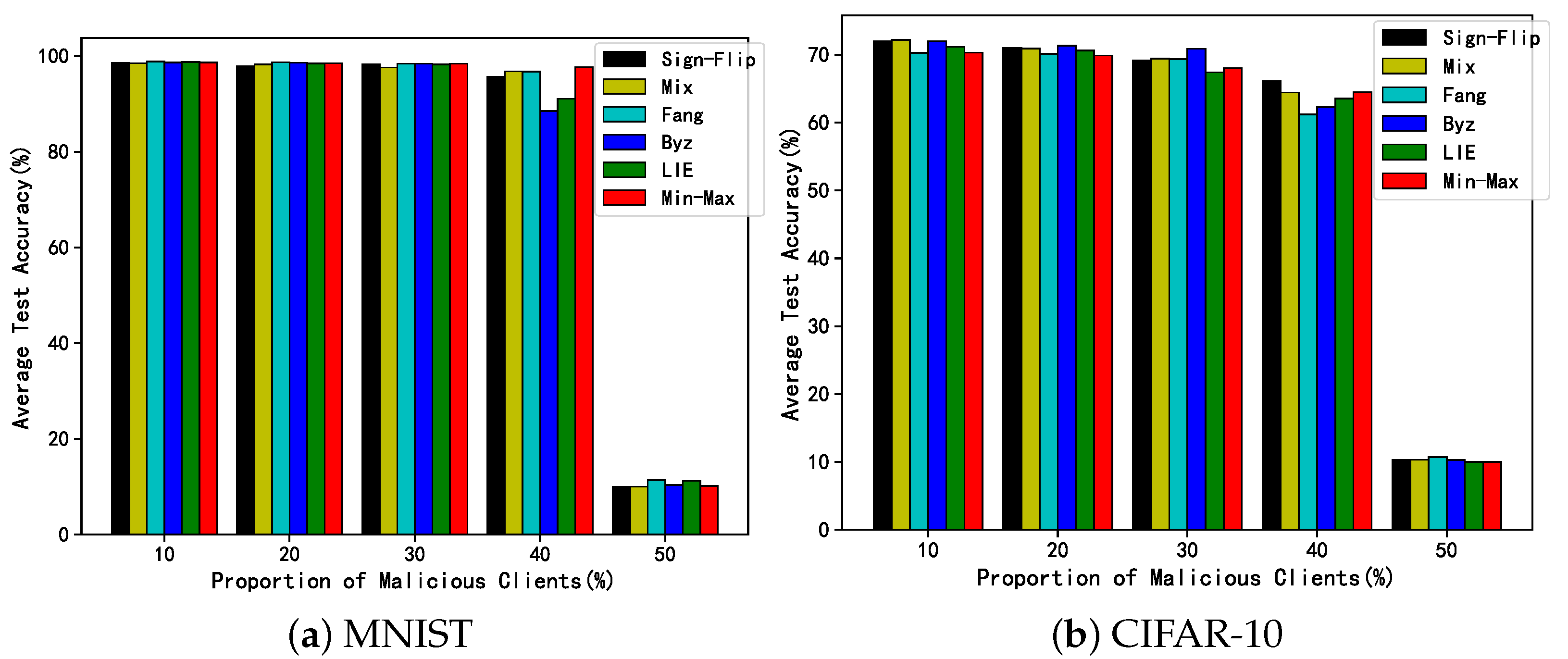
6.2.2. Comparison of Robustness among Different Aggregation Methods

To compare the robustness of various aggregation methods, this study selected the MNIST and CIFAR10 datasets and set the proportion of malicious clients between 44% and 48%.

In other words, out of 50 clients, 22 to 24 clients were randomly selected as attackers, simulating scenarios with a large number of malicious clients simultaneously conducting poisoning attacks. As shown in Figure 3 and Figure 4, under various attacks, different aggregation methods exhibited significant differences in test accuracy. For sign-flipping attacks, regardless of the dataset, FLRAM consistently outperformed other strategies. When facing Mix attacks, FLRAM maintained high accuracy. However, the Krum method did not perform well in this attack scenario. The reason is that Mix attacks allow attackers random scaling of gradients, with multiple attackers concurrently sending gradients at different scaling levels. This can lead to Krum aggregation favoring the scaled gradients, making it challenging to counter this attack. Regarding Fang attacks, due to their intricate design, both Krum and Trimmed Mean saw decreases in accuracy. In contrast, FLRAM still demonstrated high model accuracy. In addition, in Byz attacks, Krum’s performance also lagged behind other methods. In the face of LIE attacks, while FLRAM continued to maintain high accuracy, other methods experienced varying degrees of performance degradation, highlighting the severe challenges posed by more covert and destructive attacks on aggregation methods. In Min-Max attacks, FLRAM defense effectiveness was on par with the Dnc method specifically designed for this attack. Although FLAME performed well under multiple attacks, its accuracy slightly decreased due to the adoption of differential privacy techniques to enhance the privacy protection of local data.

Additionally, it can be observed that in the absence of any defense mechanism, FedAvg experiences a gradual decrease in model accuracy with increasing iterations under different attack patterns. Compared to some aggregation strategies equipped with defense mechanisms, FedAvg exhibits significantly slower convergence, emphasizing the importance of robust aggregation methods in countering poisoning attacks. When confronted with various attacks, FLRAM consistently maintains a high model accuracy, further confirming its superior robustness compared to other aggregation strategies.

6.2.3. Reliability Verification of FLRAM

To validate the reliability of FLRAM, experiments were conducted across various datasets and attack strategies with different numbers of malicious clients, as depicted in Figure 5. When selecting malicious clients, 5, 10, 15, 20, and 25 clients were randomly chosen, respectively. The results demonstrate that for both the MNIST and CIFAR10 datasets, as long as the proportion of malicious clients does not exceed 50%, FLRAM exhibits remarkable stability when facing various attacks. In the attack model assumption, the number of malicious clients should not exceed 50% of all clients. Thus, under this setting, FLRAM demonstrates robustness for the MNIST and CIFAR10 datasets. It is worth noting that in the case of Fang and Byz attacks, there is a slight decrease in accuracy when confronting 40% malicious attackers. However, overall, its test accuracy remains at a high level. This underscores FLRAM’s effective resilience against different attack strategies to a significant extent.

6.2.4. Validity under Non-IID

In practical applications, data among clients often exhibit distributional differences, a phenomenon referred to as data heterogeneity. To simulate such data heterogeneity among clients, two data allocation methods were employed: IID allocation for a portion of the total dataset, and Non-IID allocation for the remaining portion. The specific procedure is as follows: first, the training data are sorted according to labels and partitioned into different blocks based on the labels. Then, in each block, a proportion of data is extracted and distributed evenly among all clients. Subsequently, in the remaining dataset, each client can randomly obtain data from different labeled blocks. For example, some clients may only receive data for one type of label, while others may receive data for all labels, resulting in non-uniform data distribution among the clients.

Parameter s can be used to measure the degree of data heterogeneity. When s = 0, it indicates complete data heterogeneity among clients. To evaluate the impact of data heterogeneity on FLRAM, four different settings are selected: s = 0, 0.2, 0.5, and 0.8, and corresponding experiments are conducted. The experimental results are presented in

Table 3. Accuracy of Different Data Heterogeneity Levels Against Various Attacks on MNIST.

Heterogeneity(s)	0	0.2	0.5	0.8
Sign-flip	97.59	97.91	98.02	98.34
Mix	97.19	97.82	97.93	98.24
Fang	96.98	97.28	97.96	98.23
Byz	96.96	97.57	97.92	98.19
LIE	96.59	97.18	97.72	98.03
Min-Max	94.89	96.13	96.95	97.79

and

Table 4. Accuracy of Different Data Heterogeneity Levels Against Various Attacks on CIFAR10.

Heterogeneity(s)	0	0.2	0.5	0.8
Sign-flip	60.14	63.26	66.79	69.37
Mix	61.45	63.50	68.71	69.60
Fang	60.59	63.42	65.38	69.32
Byz	60.89	65.65	67.43	69.21
LIE	59.98	62.82	65.49	69.43
Min-Max	58.48	61.35	64.82	68.56

. From the tables, it can be observed that even in the case of Non-IID data, FLRAM continues to perform well in various attack scenarios.

6.2.5. Efficiency Analysis of FLRAM

FLRAM combines two methods, isolation forest and IDBSCAN, to identify anomalous gradients. Isolation forest primarily focuses on detecting abnormal gradient magnitudes, while IDBSCAN identifies anomalous gradients by clustering gradient signs. Assuming the total number of clients is n, the time complexity of anomalous gradient detection is mainly determined by the time complexity of isolation forest and the clustering time complexity of IDBSCAN. In isolation forest, the average time complexity is $O(nlog(n\left)\right)$. During the IDBSCAN clustering process, the time complexity for density similarity calculation is $O\left(n^2\right)$, density-reachable neighborhood queries are $O(nlog(n\left)\right)$, and neighborhood expansion and cluster partitioning are both $O(nlog(n\left)\right)$. Therefore, the average time complexity of IDBSCAN is $O\left(n^2\right)$. The overall average time complexity for abnormal gradient detection is $O(n^2+nlog\left(n\right))$. In a single iteration, the FLRAM average time complexity is indeed higher than that of some aggregation methods, such as Krum ($O\left(n^2\right)$) and Trimmed Mean ($O\left(nd\right)$), where d is the gradient dimension. However, as shown in Figure 3 and Figure 4, FLRAM exhibits rapid convergence characteristics. After approximately 20 rounds of iteration, the training model accuracy of FLRAM stabilizes, indicating that its higher time complexity is compensated in practical applications, achieving desirable training results in fewer iterations.

6.3. Extended Discussion

Comparison with Existing Research. When confronted with more covert and destructive attacks, the defense performance of existing research experiences a noticeable decline, whereas FLRAM’s defense performance remains robust, effectively withstanding various attacks and demonstrating superior resilience. FLRAM not only performs superbly in defense, but also offers a novel approach. It combines isolation forest and IDBSCAN to detect anomalous gradients. This method is relatively recent in the current research landscape, offering fresh solutions to address the challenges in this domain.

Time complexity. FLRAM exhibits a relatively higher time complexity in anomalous gradient detection compared to existing methods. Therefore, in future research, we will consider further optimizing the execution time of the IDBSCAN algorithm in anomalous gradient detection to enhance the efficiency and performance of FLRAM.

Novel Attack Types. FLRAM is an advanced defense method, but it cannot guarantee full resilience against unknown or novel attack types. Attackers may continuously evolve their strategies to evade FLRAM detection.

Proportion of malicious clients. Assuming that the number of malicious clients should not exceed 50% of all clients, under this premise, FLRAM demonstrates exceptional defense performance and higher reliability. However, if the number of malicious clients surpasses that of benign clients, FLRAM may struggle to effectively counter the current attacks, leading to a significant decline in its defensive performance. To address this situation, continuous learning can be employed to enhance the detection capabilities of anomalous gradients. Additionally, the selection ratio for obtaining benign gradient sets can be dynamically adjusted to maintain a higher level of defense performance.

7. Conclusions

This paper proposes a federated learning robust aggregation method known as FLRAM designed to address the challenges posed by poisoning attacks during model training. These attacks often result in model training slow convergence, failure to achieve convergence, and a reduction in model accuracy. FLRAM employs a combined approach of isolation forest and an improved density-based clustering algorithm for abnormal gradient detection for detecting anomalous gradients. It effectively filter out gradients that exhibit significant differences in magnitude and angular deviation, and then removes them. Subsequently, FLRAM employs a credibility scoring mechanism to assess the trustworthiness of each client effectively, selecting those with higher credibility. These selected clients are then aggregated to generate a global model. The experimental results demonstrate that FLRAM exhibits robust defense performance across different datasets and various types of poisoning attacks. In comparison to existing defense methods, including Krum, Trimmed Mean, RSA, FLTrust, Dnc, and FLAME, FLRAM displays higher robustness. In scenarios where the proportion of malicious clients does not exceed 50%, FLRAM shows excellent reliability in the face of various attacks, and is suitable for the scenario of Non-IID data. These results emphasize that FLRAM serves as an efficient defense method, capable of delivering exceptional performance in complex federated learning environments.

In terms of future work, there are plans to apply FLRAM to practical scenarios for poisoning attack detection to further validate its real-world effectiveness. Additionally, efforts will be made to further optimize the IDBSCAN algorithm to reduce the algorithm’s average time complexity.

References

1. McMahan, B.; Moore, E.; Ramage, D.; Hampson, S.; Arcas, B.A.Y. Communication-efficient learning of deep networks from decentralized data. In Proceedings of the Artificial Intelligence and Statistics, Fort Lauderdale, FL, USA, 22–27 April 2017; pp. 1273–1282. [Google Scholar]
2. Wu, N.; Farokhi, F.; Smith, D.; Kaafar, M.A. The value of collaboration in convex machine learning with differential privacy. In Proceedings of the 2020 IEEE Symposium on Security and Privacy (SP), San Francisco, CA, USA, 18–21 May 2020; pp. 304–317. [Google Scholar]
3. Lee, Y.; Park, S.; Kang, J. Security-Preserving Federated Learning via Byzantine-Sensitive Triplet Distance. arXiv 2022, arXiv:2210.16519. [Google Scholar]
4. Hong, S.; Chandrasekaran, V.; Kaya, Y.; Dumitraş, T.; Papernot, N. On the effectiveness of mitigating data poisoning attacks with gradient shaping. arXiv 2020, arXiv:2002.11497. [Google Scholar]
5. Gosselin, R.; Vieu, L.; Loukil, F.; Benoit, A. Privacy and security in federated learning: A survey. Appl. Sci. 2022, 12, 9901. [Google Scholar] [CrossRef]
6. Li, H.; Li, C.; Wang, J.; Yang, A.; Ma, Z.; Zhang, Z.; Hua, D. Review on security of federated learning and its application in healthcare. Future Gener. Comput. Syst. 2023, 144, 271–290. [Google Scholar] [CrossRef]
7. Lyu, L.; Yu, H.; Yang, Q. Threats to federated learning: A survey. arXiv 2020, arXiv:2003.02133. [Google Scholar]
8. Chen, Y.; Gui, Y.; Lin, H.; Gan, W.; Wu, Y. Federated learning attacks and defenses: A survey. In Proceedings of the 2022 IEEE International Conference on Big Data (Big Data), Osaka, Japan, 18–20 December 2022; pp. 4256–4265. [Google Scholar]
9. Yin, D.; Chen, Y.; Kannan, R.; Bartlett, P. Byzantine-robust distributed learning: Towards optimal statistical rates. In Proceedings of the International Conference on Machine Learning, Stockholm, Sweden, 10–15 July 2018; pp. 5650–5659. [Google Scholar]
10. Blanchard, P.; El Mhamdi, E.M.; Guerraoui, R.; Stainer, J. Machine learning with adversaries: Byzantine tolerant gradient descent. Adv. Neural Inf. Process. Syst. 2017, 30, 10. [Google Scholar]
11. Guerraoui, R.; Rouault, S. The hidden vulnerability of distributed learning in byzantium. In Proceedings of the International Conference on Machine Learning, Stockholm, Sweden, 10–15 July 2018; pp. 3521–3530. [Google Scholar]
12. Muñoz-González, L.; Co, K.T.; Lupu, E.C. Byzantine-robust federated machine learning through adaptive model averaging. arXiv 2019, arXiv:1909.05125. [Google Scholar]
13. Tolpegin, V.; Truex, S.; Gursoy, M.E.; Liu, L. Data poisoning attacks against federated learning systems. In Proceedings of the Computer Security–ESORICS 2020: 25th European Symposium on Research in Computer Security, ESORICS 2020, Guildford, UK, 14–18 September 2020; pp. 480–501. [Google Scholar]
14. Bilgin, Z. Anomaly Localization in Model Gradients Under Backdoor Attacks against Federated Learning. arXiv 2021, arXiv:2111.14683. [Google Scholar]
15. Liu, Y.; Li, Z.; Pan, S.; Gong, C.; Zhou, C.; Karypis, G. Anomaly detection on attributed networks via contrastive self-supervised learning. IEEE Trans. Neural Netw. Learn. Syst. 2021, 33, 2378–2392. [Google Scholar] [CrossRef] [PubMed]
16. Zhang, Z.; Cao, X.; Jia, J.; Gong, N.Z. FLDetector: Defending federated learning against model poisoning attacks via detecting malicious clients. In Proceedings of the 28th ACM SIGKDD Conference on Knowledge Discovery and Data Mining, Washington, DC, USA, 14–18 August 2022; pp. 2545–2555. [Google Scholar]
17. Zhao, Y.; Chen, J.; Zhang, J.; Wu, D.; Blumenstein, M.; Yu, S. Detecting and mitigating poisoning attacks in federated learning using generative adversarial networks. Concurr. Comput. Pract. Exp. 2022, 34, e5906. [Google Scholar] [CrossRef]
18. Zhu, W.; Zhao, B.Z.H.; Luo, S.; Deng, K. MANDERA: Malicious Node Detection in Federated Learning via Ranking. arXiv 2021, arXiv:2110.11736. [Google Scholar]
19. Li, L.; Xu, W.; Chen, T.; Giannakis, G.B.; Ling, Q. RSA: Byzantine-robust stochastic aggregation methods for distributed learning from heterogeneous datasets. In Proceedings of the AAAI Conference on Artificial Intelligence, Vancouver, BC, Canada, 20–27 February 2019; pp. 1544–1551. [Google Scholar]
20. Cao, X.; Fang, M.; Liu, J.; Gong, N.Z. Fltrust: Byzantine-robust federated learning via trust bootstrapping. arXiv 2020, arXiv:2012.13995. [Google Scholar]
21. Lesouple, J.; Baudoin, C.; Spigai, M.; Tourneret, J.Y. Generalized isolation forest for anomaly detection. Pattern Recognit. Lett. 2021, 149, 109–119. [Google Scholar] [CrossRef]
22. Chen, H.; Liang, M.; Liu, W.; Wang, W.; Liu, P.X. An approach to boundary detection for 3D point clouds based on DBSCAN clustering. Pattern Recognit. 2022, 124, 108431. [Google Scholar] [CrossRef]
23. Xie, C.; Chen, M.; Chen, P.Y.; Li, B. Crfl: Certifiably robust federated learning against backdoor attacks. In Proceedings of the International Conference on Machine Learning, Virtual Event, 18–24 July 2021; pp. 11372–11382. [Google Scholar]
24. Panda, A.; Mahloujifar, S.; Bhagoji, A.N.; Chakraborty, S.; Mittal, P. Sparsefed: Mitigating model poisoning attacks in federated learning with sparsification. In Proceedings of the International Conference on Artificial Intelligence and Statistics, Virtual Event, 28–30 March 2022; pp. 7587–7624. [Google Scholar]
25. Nguyen, T.D.; Rieger, P.; De Viti, R.; Chen, H.; Brandenburg, B.B.; Yalame, H.; Möllering, H.; Fereidooni, H.; Marchal, S.; Miettinen, M.; et al. {FLAME}: Taming backdoors in federated learning. In Proceedings of the 31st USENIX Security Symposium (USENIX Security 22), Boston, MA, USA, 22–26 May 2022; pp. 1415–1432. [Google Scholar]
26. Yu, S.; Chen, Z.; Chen, Z.; Liu, S. DAGUARD: Distributed backdoor attack defense scheme under federated learning. J. Commun. 2023, 44, 110–122. [Google Scholar]
27. Shejwalkar, V.; Houmansadr, A. Manipulating the byzantine: Optimizing model poisoning attacks and defenses for federated learning. In Proceedings of the NDSS, Virtual Event, 21–25 February 2021. [Google Scholar]
28. Xu, J.; Huang, S.L.; Song, L.; Lan, T. Byzantine-robust federated learning through collaborative malicious gradient filtering. In Proceedings of the 2022 IEEE 42nd International Conference on Distributed Computing Systems (ICDCS), Bologna, Italy, 10–13 July 2022; pp. 1223–1235. [Google Scholar]
29. Karimireddy, S.P.; He, L.; Jaggi, M. Learning from history for byzantine robust optimization. In Proceedings of the International Conference on Machine Learning, Virtual Event, 18–24 July 2021; pp. 5311–5319. [Google Scholar]
30. Yu, H.; Yang, S.; Zhu, S. Parallel restarted SGD with faster convergence and less communication: Demystifying why model averaging works for deep learning. AAAI Conf. Artif. Intell. 2019, 33, 5693–5700. [Google Scholar] [CrossRef]
31. Li, X.; Huang, K.; Yang, W.; Wang, S.; Zhang, Z. On the convergence of fedavg on non-iid data. arXiv 2019, arXiv:1907.02189. [Google Scholar]
32. Che, C.; Li, X.; Chen, C.; He, X.; Zheng, Z. A decentralized federated learning framework via committee mechanism with convergence guarantee. IEEE Trans. Parallel Distrib. Syst. 2022, 33, 4783–4800. [Google Scholar] [CrossRef]
33. Yu, H.; Jin, R.; Yang, S. On the linear speedup analysis of communication efficient momentum SGD for distributed non-convex optimization. In Proceedings of the International Conference on Machine Learning, Boca Raton, FL, USA, 16–19 December 2019; pp. 7184–7193. [Google Scholar]
34. Alkhunaizi, N.; Kamzolov, D.; Takáč, M.; Nandakumar, K. Suppressing Poisoning Attacks on Federated Learning for Medical Imaging. In Proceedings of the International Conference on Medical Image Computing and Computer-Assisted Intervention, Singapore, 18–22 September 2022; pp. 673–683. [Google Scholar]
35. Fang, M.; Cao, X.; Jia, J.; Gong, N. Local model poisoning attacks to {Byzantine-Robust} federated learning. In Proceedings of the 29th USENIX security symposium (USENIX Security 20), Boston, MA, USA, 18–22 September 2020; pp. 1605–1622. [Google Scholar]
36. Isik-Polat, E.; Polat, G.; Kocyigit, A. ARFED: Attack-Resistant Federated averaging based on outlier elimination. Future Gener. Comput. Syst. 2023, 141, 626–650. [Google Scholar] [CrossRef]
37. Baruch, G.; Baruch, M.; Goldberg, Y. A little is enough: Circumventing defenses for distributed learning. Adv. Neural Inf. Process. Syst. 2019, 32, 37. [Google Scholar]
Figure 1. FLRAM Process.
Electronics 12 04463 g001
Figure 2. Global gradient acquisition process.
Electronics 12 04463 g002
Figure 3. The test accuracy of each approach under various attacks with 44–48% malicious clients (based on the MNIST dataset).
Electronics 12 04463 g003
Figure 4. The test accuracy of each approach under various attacks with 44–48% malicious clients (based on the CIFAR-10 dataset).
Electronics 12 04463 g004
Figure 5. The average test accuracy of FLRAM under different proportions of malicious clients.
Electronics 12 04463 g005