Article

A Software Testing Workflow Analysis Tool Based on the ADCV Method

1
School of Computer Science and Engineering, North Minzu University, Yinchuan 750021, China
2
The Key Laboratory of Images & Graphics Intelligent Processing of State Ethnic Affairs Commission, North Minzu University, Yinchuan 750021, China
*
Author to whom correspondence should be addressed.
Electronics 2023, 12(21), 4464; https://doi.org/10.3390/electronics12214464
Submission received: 5 September 2023 / Revised: 9 October 2023 / Accepted: 11 October 2023 / Published: 30 October 2023
(This article belongs to the Special Issue Big Data and Large-Scale Data Processing Applications)

Abstract

:
Based on two progressive aspects of the modeling problems in business process management (BPM), (1) in order to address the increasing complexity of user requirements on workflows underlying various BPM application scenarios, a more verifiable fundamental modeling method must be invented; (2) to address the diversification of software testing processes, more formalized advanced modeling technology must also be applied based on the fundamental modeling method. Aiming to address these modeling problems, this paper first proposes an ADCV (acquisition, decomposition, combination, and verification) method that runs through the core management links of four types of business processes (mining, decomposition, recombination, and verification) and then describes the compositional structure of the ADCV method and the design of corresponding algorithms. Then, the software testing workflow is managed and monitored using the method, and the corresponding analysis tool is implemented based on Petri nets. At the same time, the tool is applied to the case processing of the software testing workflow. Specifically, the workflow models are established successively through ADCV during the process of business iteration. Then, the analysis tool developed with the ADCV method, the model–view–controller (MVC) design pattern, and Java Swing technology are applied to instances of the software testing workflow to realize the modeling and management of the testing processes. Thus, the analysis tool can guarantee the accuracy of the parameter estimations of related software reliability growth models (SRGMs) and ultimately improve the quality of software products.

1. Introduction

In the current software operating environment, due to the complexity and diversification of user requirements, as well as the dynamicity of the runtime environment for workflow management systems, increasing importance has been attached to BPM by more and more industries [1]. Business process management is an effective means for enterprises or organizations to achieve their goals [2]. The process model is the research foundation in the field of BPM. It can not only assist in developing information management systems but can also analyze process changes and then improve the processes in question, which is helpful in managing more complex business processes. Therefore, against the background of the increasing complexity of BPM, establishing a reliable process model that can cope with dynamic changes and ensure that business processes can be carried out continuously and effectively is the principal problem in reliability modeling. Traditional process modeling methods are complex, with strong subjectivity, poor accuracy, and low execution efficiency. Moreover, in most cases, they cannot meet the actual needs of current process development. The historical data stored in information systems about process execution provide a valuable source of data for discovering and improving business processes within an organization. Running business processes consists of different activities that form log data.
Usually, the software reliability growth model (SRGM) is used as a basic tool to predict or evaluate the reliability of software products in the software testing stage, and the application of SRGM for reliability analysis is also an effective means in the field of reliability evaluation [3]. With the constant expansion of software system scales, software functions require more frequent interaction among various subsystems, and their reliability is often difficult to predict. Therefore, before the software system is delivered to users, it is necessary to carry out fault detection and fault repair according to a reliable software testing process so as to avoid failure behaviors during the actual operation process.
In this paper, we propose an automated workflow modeling architecture based on the ADCV method for the primary research BPM modeling tool used in software testing. The workflow models are established successively according to the methods of acquisition, decomposition, combination, and verification, which provide reliable model guarantees for software testing processes and, consequently, improve the quality of BPM in software testing. The process logs record the real execution situation of the business process. By mining the logs’ information, the process acquisition component initially establishes a Petri nets model that conforms to the corresponding process log. After the process model is decomposed by the process decomposition component, the sublogs and submodels are generated, and the original Petri nets model is decomposed into several models. According to changes in business requirements, the original business process needs to be recombined, updated, and optimized; then, the process recombination is implemented with the participation of users. Finally, the new model is compared with the original model through the process verification component to determine the reachability and the differences between the places, thus completing the property analysis of the model.
The remainder of this paper is organized as follows: First, we introduce some related work in Section 2, i.e., Petri nets and software testing workflows, the Petri nets model of the fundamental workflow mode, and tool architecture and functions. In Section 3, we discuss business process analysis based on the ADCV method and the corresponding process mining algorithm. Section 4 applies the ADCV method to the modeling of a real software testing process. The last section provides a research overview and the future research direction of this paper.

2. Related Work

2.1. Petri Nets and Software Testing Workflow

Petri nets are often used for modeling, simulation, control, and analysis of automated manufacturing systems [4,5]. The method of workflow modeling based on Petri nets is more and more widely applied in BPM and can provide technologies and means for the structure analysis and performance evaluation of workflow models. With the expansion of software scales, more software failures occur, and the importance of software testing is becoming more prominent. The application of Petri nets in the BPM field of software testing can effectively carry out formal analysis and testing for software, thus reducing the testing cost and improving testing efficiency. However, in the testing stage of software development, SRGM describes the cumulative number of faults detected or repaired during the software testing process based on historical failure data, which plays an important role in the reliability evaluation and safety measurement of the software system [6,7]. Obviously, when the faults in software are continuously eliminated, the software reliability will be improved.
In general, after the software development is completed, we establish the corresponding SRGM from the perspective of software failures in the software testing process or actual delivery and execution to obtain the reliability measurement results of the software [8,9]. However, in order to accurately find the root cause of software failures, we need a high-quality software testing process. Therefore, an accurate analysis of the key factors affecting the SRGM of the tested software in the software testing process is helpful in establishing a more accurate SRGM of the tested software. Through formal Petri nets modeling for the software testing process, we improve the automation of the software testing workflow. Furthermore, we obtain more accurate reliability measurement results of the tested software. Applying SRGM in software testing can not only provide reliable information about the tested software for testers but also help to establish the best software release decision and further improve the software quality.

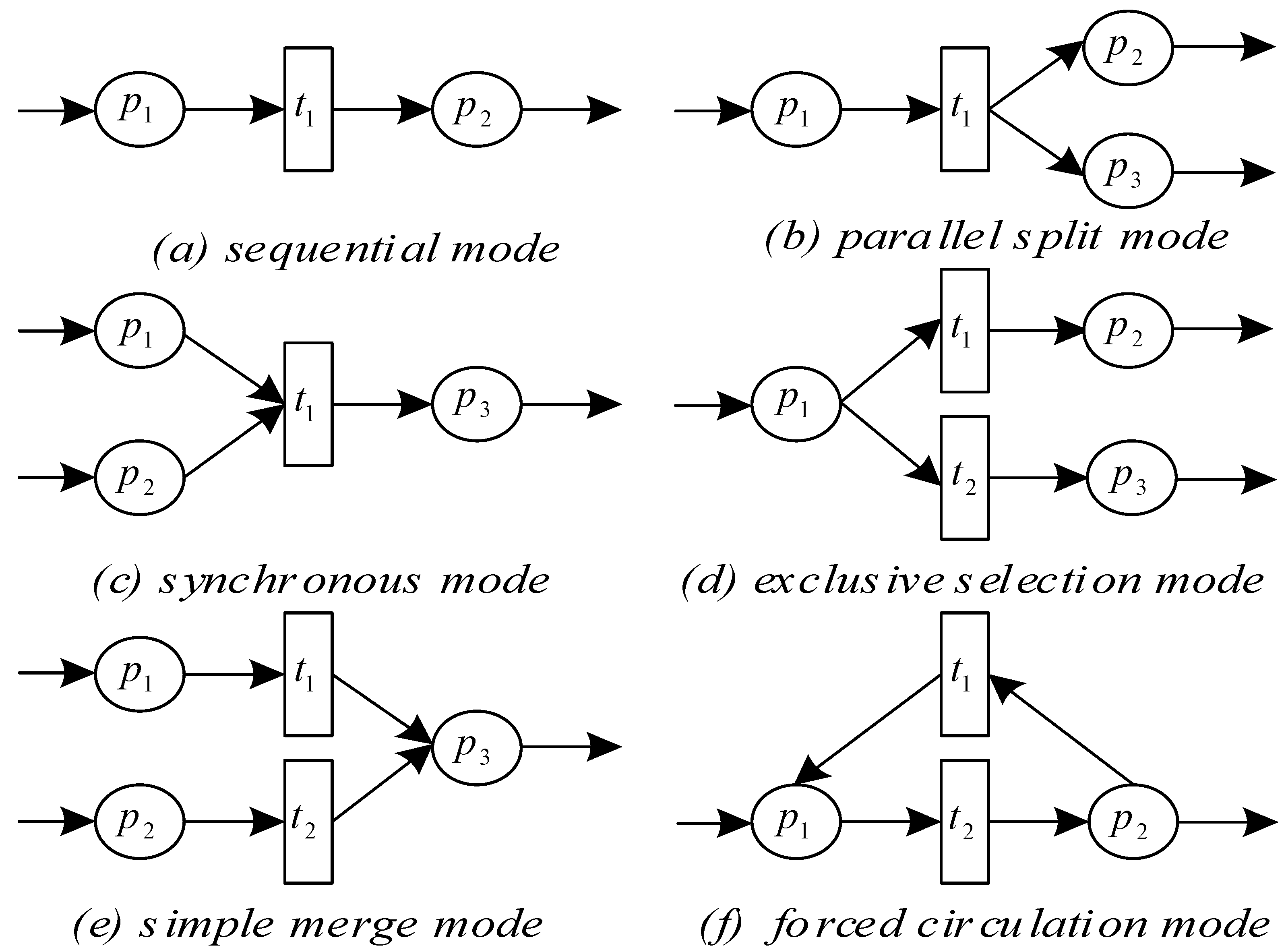
2.2. Petri Nets Model of the Fundamental Workflow Mode

Workflow separates management from business processes and makes business and BPM independent to realize the automation of BPM. On the basis of Petri nets, Wil van der Aalst proposed the theory of workflow-net (WF-net) by modeling the control flow dimension of a workflow [10]. As a kind of Petri net, WF-net is widely used in workflow system modeling and analysis [11,12,13]. A WF-net begins at the initial place and ends at the termination place, which indicates the running state of a complete business process under the marking. Workflow modeling can be completed by using Petri nets, and the Petri nets models corresponding to the fundamental workflow modes are shown in Figure 1.
Figure 1a–f corresponds to sequential mode, parallel split mode, synchronous mode, exclusive selection mode, simple merge mode, and forced circulation mode, respectively. Among them, Figure 1a,d,f correspond to the sequential model, selective model, and cycle model, respectively, while Figure 1b–e belong to the parallel model. According to the above four basic Petri nets models, we can model and analyze the business process of workflow to optimize the workflow management system and improve the quality of BPM.

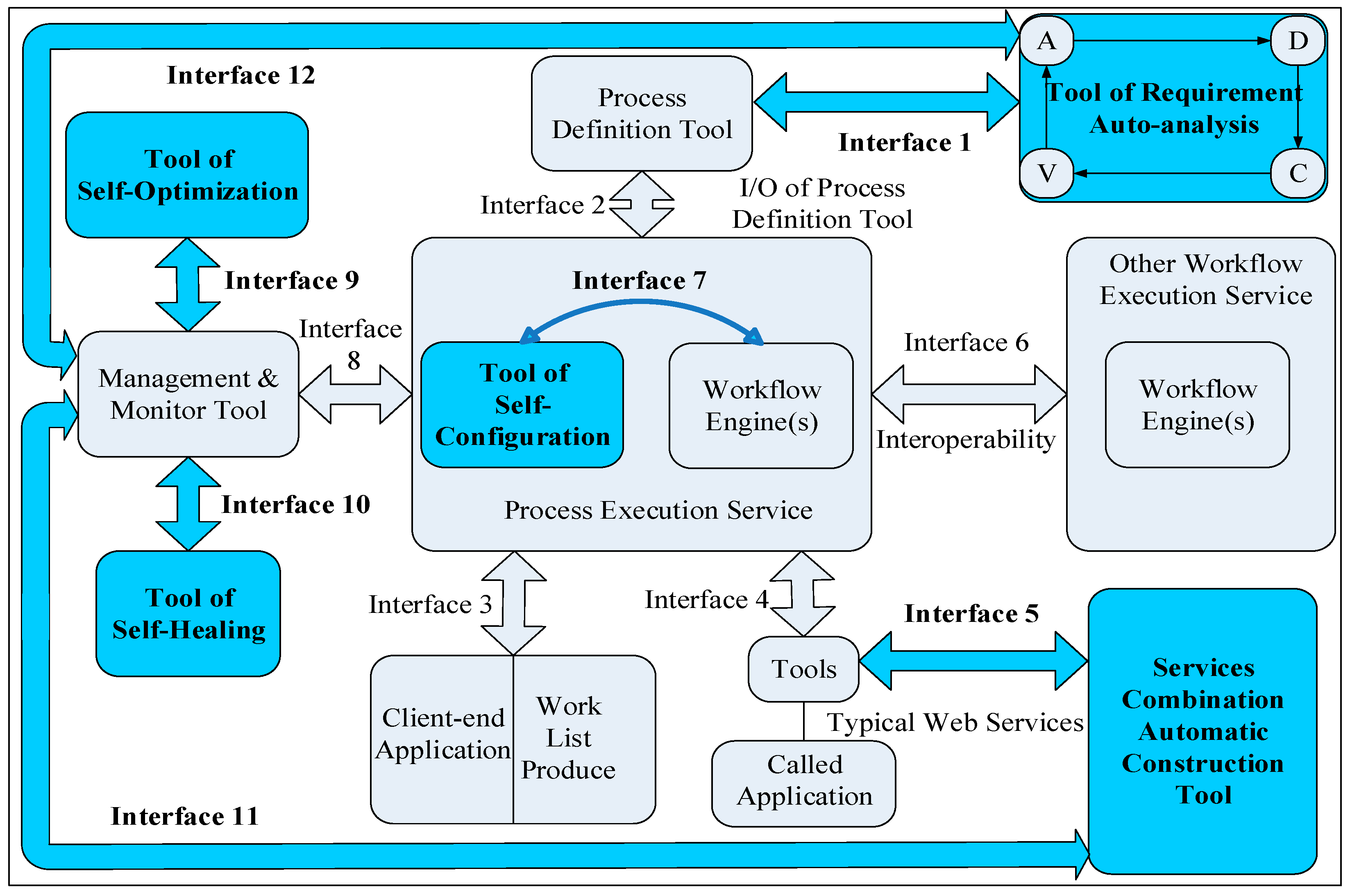
2.3. Architecture and Functions of Tool Based on ADCV Method

With the support of WfMS (workflow management system), the advantages of BPM application software, such as high flexibility and maintainability, have been widely accepted by users. Moreover, workflow management software promotes the rapid development of process management concepts such as process recombination and continuous process improvement. In addition, these management concepts also speed up process optimization and improve the quality of process models. The trustworthy workflow management system (TWfMS) [14,15] is an extension of the standard reference model proposed by the workflow management coalition (WfMC) and links the process definition tool to the Petri nets analysis tool to automate the acquisition, decomposition, recombination, and verification of uncertain business process models, as shown in Figure 2.
At the same time, an instance of TWfMS could be established in the high-quality software testing process, which can derive the relative SRGM to reflect the results of software testing. The SRGM plays an important role in the evaluation and analysis of software reliability. With the increasing scale and complexity of software applications, the field of software reliability analysis has become increasingly prominent [16]. The functionality of complex software systems requires frequent interactions and connections between subsystems, and the complexity of the entire system will greatly increase, making its reliability often difficult to predict [17]. Therefore, it is necessary to study the concept of software reliability from the perspective of improving the software service quality.
In Figure 2, interface 1 is linked to the tool of requirement auto-analysis through the process definition tool, which can automatically acquire, decompose, combine, and verify uncertain business processes for requirement analysis. The analysis tool based on Petri nets includes the four core functions of the ADCV method, i.e., acquisition, decomposition, combination, and verification. The specific methods of this paper are described as follows:
  • A: Firstly, the process acquisition component generates the corresponding process model by mining the event logs, thus obtaining the structured business process. Here, we adopt a formal method suitable for describing concurrent systems to model, such as Petri nets.
  • D: Secondly, the process decomposition component analyzes the established simulation model and extracts the relatively stable subsystem structure, i.e., it can identify and decompose the subprocesses of structured business processes. For example, the obtained model is decomposed into multiple subnets according to the T-invariants of the Petri nets, thus forming multiple nonintersecting subprocesses represented by each subnet.
  • C: Thirdly, with the participation of users, it is inevitable that business processes will be recombined due to the changes in requirements, that is, process combination. Generally, the processes involved in the recombination are the subprocesses identified and decomposed in the second stage above, which ensures that the recombined process can better reflect the new requirements.
  • V: Finally, the process verification component performs formal verification on the recombined process model to determine whether it meets the new requirements. Regarding the processes that proved to be unable to meet the new requirements after verification, we need to feed back the requirements analysis reports to the first stage, that is, the modeling stage, to participate in the process acquisition again and enter a new round of the iterative cycle of BPM.

3. Business Process Analysis Based on the ADCV Method

3.1. Overview of the ADCV Method

Figure 3 shows the key elements, key technologies, and key steps of the ADCV method. The key elements include the BPMN (business process model and notation) model, WfMS, event log, sublog, subnet, and model, etc.; the key technologies include process mining, process decomposition, process recombination, and process verification, etc.; the key steps include development, discovery, decomposition, comparison, combination, recombination, verification, and design, etc.
In Figure 3, firstly, WfMS development should follow the specifications of the BPMN model; after the BPMN model is converted to the workflow net model, it should satisfy the characteristics of being well-structured and reasonable. The event log is generated from the actual running process of the WfMS; then, the process mining technology is used to discover the model M1 from the log data, and the M1 is decomposed to generate the subnet model set M2. The sublog set is generated by decomposing the logs, and these sublogs are separately discovered to obtain the subnet model set M2. Next, we compare the corresponding subnet models in M2 and M2 and recombine the BPMN model with subnet 1, subnet 2 ··· subnet n in terms of the decomposition results reached by the consensus after comparison to generate the model M3. Finally, the verified model M4 is submitted to the user, who can redesign the original BPMN model and update the WfMS iteratively.
Figure 4 outlines the detailed modeling relationship of the ADCV method; that is, this paper establishes the workflow model in turn according to this method and continuously carries out the iterative cycle of business process modeling in accordance with user requirements until the generated new model (M4) is accepted by users. Business process modeling and analysis based on the four major phases of the ADCV method aims to consistently improve the quality of business process management.

3.2. Business Process Acquisition

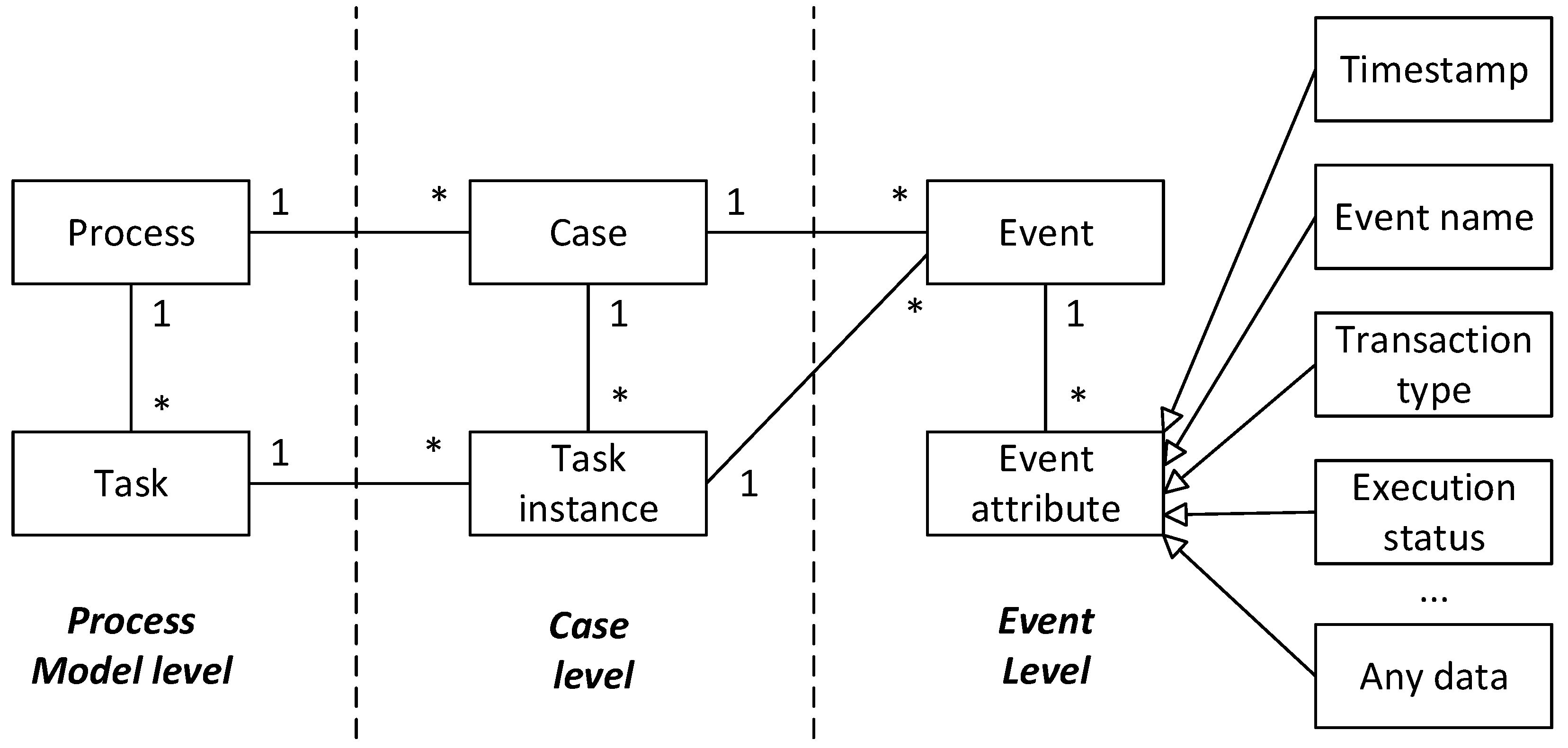
3.2.1. Log Definition Based on Event Status

The log data recorded by the information system may reside in multiple database tables. The log data information may contain one or more events and provide the corresponding event name, start time, end time, execution status, etc. The same process model can contain multiple process instances, and different process instances may contain different events. We replay the event log on the process model; that is, we convert the event log into a visual process model, and the events in the log are closely related to the tasks in the model. Figure 5 shows the process of establishing a connection between the process model and the event log when the log is replayed and connects the processes and activities in the model to the events in the log. The process mainly involves three levels: process model level, case level, and event level.
In Figure 5, the event is connected to the task instance so that the data information in the log can be projected onto the process model. For the purpose of more accurately describing the log based on the event status adopted in this work and facilitating the analysis of the log, the following definitions are given:
Definition 1 (log based on event status).
Different from the traditional event log format, the log format used in this paper mainly has three attributes: CaseId, EventName, and EventStatus, wherein the CaseId indicates the Id number of the workflow case (represented by serial numbers 1, 2, 3,  ···), that is, the Id number of the trace sequence in a log; the EventName indicates the name of the event contained in the trace sequence; the EventStatus indicates the event status, including start (abbreviated as S) and complete (abbreviated as C), which indicate the start status and complete status of an event, respectively.
The traditional event log format treats a task as an atomic activity and does not involve the specific start and complete status of events. However, we consider event status as a major factor in log attributes. Table 1 shows a complete log containing the event status S and C, which records the software testing workflow of RSA timing attack tasks in detail. The RSA encryption algorithm was proposed by Rivest, Shamir, and Adleman in 1977. The RSA timing attack tasks refer to using time-side channels to attack RSA keys. Then, the attacker collects the time information generated by the RSA algorithm when processing different ciphertexts and uses multivariate statistical analysis methods to crack the keys [18,19].
The event log in Table 1 includes four workflow cases, of which the trace sequence corresponding to case 1 is:
σ 1 = < ( t 1 , S ) , ( t 1 , C ) , ( t 2 , S ) , ( t 2 , C ) , ( t 4 , S ) , ( t 4 , C ) , ( t 5 , S ) , ( t 5 , C ) , ( t 6 , S ) , ( t 6 , C ) , ( t 11 , S ) , ( t 7 , S ) , ( t 11 , C ) , ( t 12 , S ) , ( t 7 , C ) , ( t 8 , S ) , ( t 8 , C ) , ( t 12 , C ) , ( t 13 , S ) , ( t 13 , C ) , ( t 14 , S ) , ( t 14 , C ) , ( t 15 , S ) , ( t 15 , C ) >
where ( t 1 , S ) and ( t 1 , C ) represent the start event and complete event of task t 1 in an instance, respectively. On the one hand, for t i σ , ( t i , S ) and ( t i , C ) must appear in pairs, and ( t i , S ) can only appear before ( t i , C ) . On the other hand, events such as t 7 and t 11 in case 1, t 9 and t 11 in case 2, and t 8 and t 12 in case 3 overlap when they are executed, respectively, indicating that there may be a parallel execution relation between these tasks in case 1, 2, and 3. Furthermore, each event (start event or complete event) in a trace only corresponds to the occurrence of the same task, and a task may appear in the log more than once due to the loop structure. To formally describe the relation between tasks in the log, the definitions of the two basic inter-task relations used to derive the ordering relations between tasks are given below.
Definition 2 (succession and intersection).
Let T  represent the set of tasks, E = T × { S t a r t , C o m p l e t e }   represent the set of events on T  (including the start and complete events of all tasks), and L E *   (i.e., L P ( E * ) ; P ( E * )   is the powerset of E * ), which represent an event log. In log L , a , b , c T   represents three tasks:
(i) 
If, and only if, events ( a , S ) , ( a , C ) , ( b , S ) , ( b , C )   have occurred in a trace σ E *   and satisfy ( a , C ) . t i m e s t a m p < ( b , S ) . t i m e s t a m p   (i.e., a   has been completed before b   starts), that is, if there is at least one trace in the log, and no complete task c   occurs between its two tasks a   and b , then a   is directly succeeded by b , which is represented by a > L b .
(ii) 
If, and only if, events ( a , S ) , ( a , C ) , ( b , S ) , ( b , C )  have occurred in a trace σ E *  and satisfy ( a , S ) . t i m e s t a m p < ( b , S ) . t i m e s t a m p < ( a , C ) . t i m e s t a m p  or ( b , S ) . t i m e s t a m p <   ( a , S ) . t i m e s t a m p < ( b , C ) . t i m e s t a m p , that is, if there is at least one trace in the log, and its two tasks a  and b  overlap and intersect, then a  intersects with b , which is represented by a × L b .
Figure 6 shows the situations of a > L b and a × L b . As can be seen from Figure 6, the two tasks with intersection relation are bound to be parallel. The difference is that the completion sequence is different; that is, a × L b and b × L a both believe that the execution process of tasks a and b is parallel, and the two situations of a × L b indicate that the start sequence of the two tasks is different. Similarly, the two situations of b × L a indicate that the start sequence of the two tasks is different. Meanwhile, on the premise that the log is complete, a × L b and b × L a are equivalent; that is, a × L b b × L a . After establishing the basic relations such as > L and × L , this work extends the following three types of ordering relations between tasks to construct the model structures that conform to the log behaviors.
Definition 3 (log-based ordering relations).
Let L E *  be an event log based on E = T × { S t a r t , C o m p l e t e } . For a , b T :
(i) 
Causal relation: a L b  iff ( a > L b ) ¬ ( b > L a ) ¬ ( a × L b ) ¬ ( b × L a ) ;
(ii) 
Indirect relation: a # L b  iff ¬ ( a > L b ) ¬ ( b > L a ) ;
(iii) 
Parallel relation: a | | L b  iff ( a > L b ) ( b > L a ) ( a × L b ) ( b × L a ) .
For any log L , if a , b T , then the task pair ( a , b ) T × T consisting of a and b must satisfy and only satisfy one of the following four relations: a L b , b L a , a # L b , and a | | L b ; i.e., these relations constitute the partition of the set T × T . According to the above definitions, it can be concluded that parallel and indirect relations conform to exchangeability, while causal relation does not.

3.2.2. αS Algorithm Based on Event Status

Process mining is a technique for extracting useful information from workflow logs and providing an interface between process models and event data [20], which is used by many data-driven organizations to improve performance or ensure compliance [21]. In the application of the α algorithm, the task in the log is considered an atomic activity, and the execution status of the task (the start status and complete status) is not considered, which is not conducive to the detection of the parallel relation between tasks. Therefore, the improved αS algorithm based on the α algorithm in this paper regards the start and complete events of a task as two atomic activities and explicitly detects the parallel structures in the business process by recording the occurrence of overlapping tasks. In addition, the αS algorithm overcomes the problem that the α algorithm cannot correctly handle the short loops (loop structure with step 1 or 2) and further improves the applicability of process mining technology in practical situations.
Next, let L be an event log based on E = T × { S t a r t , C o m p l e t e } . The steps of the αS algorithm are as follows:
Step 1:  T L = { t T | σ L t σ }
Step 2:  T I = { t T | σ L t = f i r s t ( σ ) }
Step 3:  T O = { t T | σ L t = l a s t ( σ ) }
Step 4: X L = { ( P S i , N S i )   P S i T L N S i T L a P S i b N S i a L b a 1 , a 2 P S i a 1 # L a 2 b 1 , b 2 N S i b 1 # L b 2 }
Step 5:  Y L = { ( P S i , N S i ) X L | ( P S i , N S i ) X L P S i P S i N S i N S i ( P S i , N S i ) = ( P S i , N S i ) }
Step 6:  P L = { p ( P S i , N S i ) | ( P S i , N S i ) Y L } { i L , o L }
Step 7:  F L = { ( a , p ( P S i , N S i ) ) | ( P S i , N S i ) Y L a P S i } { ( p ( P S i , N S i ) , b ) | ( P S i , N S i ) Y L b N S i } { ( i L , t ) | t T I } { ( t , o L ) | t T O }
Step 8:  α S ( L ) = ( P L , T L , F L ) .
Then, the triple ( P L , T L , F L ) is the process model constructed by the αS algorithm based on log L . Step 1 is responsible for detecting all the tasks in the log, and these tasks should correspond to the transitions in the resulting Petri nets model. In steps 2 and 3, T I is the set of tasks that appears at the first position of a trace and T O is the set of tasks that appears at the last position of a trace. As the cores of this algorithm, step 4 and step 5 play significant roles in process mining. Step 4 tries to find the set X L formed by all task pairs ( P S i , N S i ) under certain conditions, and there is a causal relation between each task in the set P S i and each task in the set N S i ; moreover, there are no parallel or causal relations between the tasks of P S i and N S i ; that is, there is an indirect relation, which is important for finding the short loop structures in log records. Step 5 removes all sets in X L that do not contain the largest elements to generate Y L . In step 6, each task pair ( P S i , N S i ) has a place p ( P S i , N S i ) corresponding to it, which is used to connect the transitions in P S i and N S i ; furthermore, a Petri nets model should also contain an initial place i L and a termination place o L . Step 7 is responsible for generating the directed arc between the place and transition in the Petri nets model. All places p ( P S i , N S i ) take P S i as the input transition and N S i as the output transition and finally construct a complete Petri nets model α S ( L ) = ( P L , T L , F L ) in Step 8.

3.3. Business Process Decomposition

3.3.1. Principle of Process Decomposition

By using the process mining algorithm to detect and analyze the event log, the Petri nets model that can replay the log behaviors can be obtained. However, the complexity of business processes is further expanding, which, on the one hand, brings some challenges to the performance analysis of related processes; on the other hand, it may cause the state space of the Petri nets model to increase exponentially and then lead to a state space explosion. In order to alleviate the problem of the state space explosion, the strategy of “divide and conquer” can be adopted; that is, the net structure or state space of the model can be divided by employing process decomposition technology. Thus, the original model can be decomposed into several subnet models. This section mainly discusses the combination of process decomposition technology and process mining technology to decompose the process mining problem into multiple small-scale problems to reduce the difficulty of process discovery and improve the quality of the process model. Additionally, these small-scale problems are easy to analyze, and the decomposition results can be recombined to form the original problem.

3.3.2. Process Decomposition Algorithm Based on T-Invariant

On the basis of understanding and mastering the relevant theories of process mining, we present a process decomposition algorithm based on the T-invariant, which can effectively realize the separation of business processes. Let L be an event log based on E = T × { S t a r t , C o m p l e t e } , which was derived from the execution records of a WfMS. The WfMS was designed and implemented in terms of a well-structured and reasonable workflow net P N = ( P , T ; F ) , where the workflow net refers to Definition 2.9 and Definition 4.2 specified in the literature [10]. Next, let L = { σ 1 , σ 2 , , σ C a s e N u m } , where C a s e N u m represents the number of workflow instances in L , and σ l ( 1 l C a s e N u m ) represents the trace of the l t h workflow instance. From the preliminary analysis of the process decomposition algorithm, the extended workflow net P N ¯ = ( P ¯ , T ¯ ; F ¯ ) is defined on the basis of the workflow net P N = ( P , T ; F ) as follows: (1) P ¯ = P ; (2) T ¯ = T { t * } ; (3) F ¯ = F { ( o , t * ) , ( t * , i ) } .
Then, the steps of the process decomposition algorithm based on the T-invariant are as follows:
Step 1: Description: The Petri nets model given by the business process acquisition link is decomposed into several subnet models.
Step 1.1: Add a new transition t * between initial place i L and a termination place o L to construct the extended workflow net P N ¯ ; i.e., t * = { o L } , t * = { i L } .
Step 1.2: Solve the output matrix D m × n + , input matrix D m × n , and incidence matrix D m × n of P N ¯ , and | P | = m , | T | = n .
Step 1.3: Solve the homogeneous linear equation D m × n X = 0 with constraint condition X > 0 to obtain a group of minimal T-invariant solutions X 1 , X 2 , , X k and their support set solutions T S 1 , T S 2 , , T S k . Let T S be the T-invariant support set, which can be expressed as T S = T S T S = { T S 1 , T S 2 , , T S k } ; T S is the T-invariant set containing transition t * , and T S is the T-invariant set without transition t * .
Step 1.4: Construct the outface subnet P N i = ( P i , T i ; F i ) of P N ¯ for T S i T S , and let T S P N be the set of outface subnets; i.e., T S P N = { P N 1 , P N 2 , , P N T S } .
Step 1.5: If T S = , then skip to Step 1.7; otherwise, T S j T S , if P N i T S P N ( T S i T S ), then T S i T S j , and p P N i t T S j , such that t = p . Then, merge the outface subnet of T S j in P N ¯ with P N i to obtain a combined extended subnet P N i . In addition, T S = T S \ T S j .
Step 1.6: Repeat Step 1.5 until the element in T S is empty ( T S = ).
Step 1.7: Delete t * and its corresponding arcs ( o , t * ) and ( t * , i ) from each extended subnet P N i , and the set W F P N = { P N 1 , P N 2 , , P N T S } of workflow subnets is constituted of these new P N i .
Step 2: Description: Based on the results of the T-invariant support sets given in Step 1, the original log is decomposed into several sublogs.
Step 2.1: Convert the T-invariant support sets of T S and T S in Step 1.3 to the transition set, respectively.
Step 2.2: Initialize S L = T S ( T S in Step 1.3), which represents the set of sublogs; initialize L _ e x c e p t i o n = , which represents the set of exception logs that cannot be replayed by the Petri nets model given in Step 1. The original log L is decomposed in terms of the transition set of T S in Step 1.3; i.e., T S i T S . If l , T S i \ t * σ l , σ l L , then S L = S L { σ l } and L = L \ σ l ; if l , T S i \ t * σ l , then L _ e x c e p t i o n = L _ e x c e p t i o n { σ l } and L = L \ σ l . Finally, the sublog set that constitutes the log L is L = { S L 1 , S L 2 , , S L T S ,   L _ e x c e p t i o n } .
Step 3: Description: Process mining technology is employed to process these sublogs separately, and the corresponding workflow subnet models are generated. Then, compare them with the subnet models obtained in Step 1 (if the comparison result is the same, retain them; otherwise, discard the subnet model). Therefore, the set of subnet models resulting from sublog mining is W F P N = { P N 1 , P N 2 , , P N T S } .
In Steps 1.4 and 1.5, T S and T S represent the T-invariant set of the outer loop execution trace and the T-invariant set of the internal loop execution trace, respectively. These two steps are the cores of the decomposition algorithm. On the one hand, they are responsible for the construction and merging of the extended subnets, preventing the loss of the loop structures in the log and model and ensuring the independent relationship among the subprocesses; on the other hand, the construction and merging of subnets need to be completed in polynomial time. In the worst case, each transition needs to establish an association relationship with each place in the P N ¯ ; therefore, the time complexity is O ( m n ) ( | P | = m , | T | = n ). Steps 1.2 and 1.3 solve homogeneous linear equations D X = 0 under the constraint condition X > 0 , which also need to be completed in polynomial time; in the worst case, the time complexity is O ( m n ) . The time complexity of steps 1.1, 1.6, 1.7, 2, and 3 is negligible compared to the above analysis. Therefore, the time complexity of the decomposition algorithm is O ( m n ) .

3.4. Business Process Combination

3.4.1. Workflow Modeling Based on Time Petri Nets

With the increasing demands for automation in the field of BPM, business process modeling has gained more and more attention from the industry. Business process modeling covers process combination and process recombination, in which process combination refers to combining some process fragments into a complete process model according to specific modeling rules, while process recombination refers to the process of redesigning existing processes based on business requirements. After the process decomposition, the original workflow net model is divided into several workflow subnet models with independent execution traces. Then, on the basis of sorting out the global business process, these subnet models are combined to form a complete workflow model, which provides a good model condition for the next process recombination modeling. The workflow net model input in the process decomposition stage is the Petri nets model obtained by using process mining technology to discover logs automatically. The goal of process combination is to use some basic elements of Petri nets to implement combination modeling for the process fragments generated after decomposition. The process of recombination is based on the decomposed subnet model to create the initial elements of the recombination model, delete the old elements, add new elements, and then establish a more reasonable Petri nets model. Therefore, we can compare the differences between the two models before and after the recombination to determine the changes in business requirements. After the process of recombination is completed, the new model is verified to check its reachability status.
In the modeling process of combination and recombination, each transition is given a fixed delay time; thus, the workflow model is associated with a time parameter to build a time Petri nets model. On the basis of time Petri nets, we add a certain amount of weight values to the directed arcs in the Petri nets model and further propose a modeling method of weighted time Petri nets to improve the overall modeling ability of the workflow model.
The time delay parameter is introduced to a Petri net, and a weighted time Petri net is defined as a seven tuple, i.e., T P N = ( P , T ; F , K , W , M 0 , D ) . Among them, D { 0 , 1 , 2 , } is the delay time set for transition, and W F T P N is the weight function on T P N . If ( p , t ) F , then W ( p , t ) is called the weight on ( p , t ) . For p t and t T , if M ( p ) 1 , it means t can be triggered under marking M to obtain a new marking M . According to the workflow net model and subnet model obtained from process acquisition and process decomposition, the weighted time Petri nets are adopted to implement the combination and recombination of a business process, which not only improves the modeling and analysis capabilities of basic Petri nets but also can simulate the dynamic changes in business processes with the help of the movement of the token in the places and the continuous running time of the transitions. The workflow modeling based on weighted time Petri nets provides an exploration method for the simulation of process models, which can better meet the actual requirements of business processes.

3.4.2. Improved Coverage Tree Algorithm

A rational Petri nets model can ensure the accuracy and reliability of the business process, but to verify whether a Petri nets model meets the rationality, it is necessary to analyze all possible state transitions of the entire model. Hence, we can use the coverage tree to describe the marking transformation process of a Petri nets model. In the coverage tree, the node represents the new marking generated by M 0 and its subsequent marking, and the directed arc represents a process in which a transition is triggered (i.e., one marking is transformed into another). However, when P N is unbounded, the state space of the coverage tree tends to infinity. Therefore, in order to keep the finiteness of the coverage tree, an infinite component ω is introduced to express the meaning of infinite. For any positive integer n , there are ω > n , ω ± n = ω , and ω ω .
Definition 4 (marking coverage).
(i) 
M 1 M 2 i M 1 ( p i ) M 2 ( p i ) .
(ii) 
M 1 < M 2 M 1 M 2 i M 1 ( p i ) < M 2 ( p i ) ,
where M : P { 0 , 1 , 2 , }  represents marking and P = { p 1 , p 2 , , p m } . Then, the marking M   can be written as a row vector; that is, M = ( M ( p 1 ) , M ( p 2 ) , , M ( p m ) ) . In definition 4, if each component M 1 ( p i )   of marking M 1  satisfies the condition that it is less than or equal to the corresponding component M 2 ( p i )  of M 2 , then M 1  is covered by M 2 ; if M 1  is covered by M 2 , and M 1 ( p i )  is less than M 2 ( p i ) , then M 1  is less than M 2 .
The traditional coverage tree algorithm has obvious shortcomings in analyzing the marking transformation process of Petri nets, which are specifically reflected as follows:
(i) The true leaf nodes are divided into live nodes and dead nodes. The corresponding transitions of live nodes can occur repeatedly, while dead nodes will not trigger any other transitions. However, these two types of nodes cannot be explicitly distinguished in a coverage tree.
(ii) A node may have two child nodes, and the transitions corresponding to these two child nodes may have concurrent or selective execution (i.e., conflict), which is also not effectively distinguishable in a coverage tree. Aiming at the above problems of the traditional coverage tree algorithm, this work proposes an improved coverage tree algorithm to construct an optimized and reasonable coverage tree model.
Next, C T ( P N ) is used to represent a coverage tree to be constructed, and P N is used to represent a known Petri nets system. In a coverage tree C T ( P N ) , the node represents the marking name, M x represents the marking of node x , and the directed arc between the parent node and the child node represents a process in which a transition is triggered.
Then, the steps of the improved coverage tree algorithm are as follows:
Step 1: Take the initial marking M 0 as the root node of C T ( P N ) ; i.e., the initial value of C T ( P N ) is M r o o t = M 0 .
Step 2: Judge whether M 0 of C T ( P N ) exists. If not, the algorithm ends; if yes, perform the following:
Step 3: If there are several enabled transitions at M 0 , choose one to trigger, mark the obtained leaf node x as a new marking M x , and judge whether x is a true leaf node.
Step 3.1: If there is no enabled transition at M x , then x is the terminal node (also called the true leaf node).
Step 3.2: If node y exists on the directed path from r o o t to x , making M y = M x , then y and x are duplicate true leaf nodes, i.e., duplicate nodes.
Step 3.3: When all the leaf nodes in C T ( P N ) meet the requirements of true leaf nodes, the algorithm ends; otherwise, go to Step 4.
Step 4: At the marking M x of a non-true leaf node x , there is an enable transition t , and a new marking M z can be obtained after it is triggered, i.e., ( P N , M x ) [ t > M z . Then, add the new node z to C T ( P N ) , establish a directed arc from x to z , and mark the arc as t .
Step 5: If there exists a node c on the directed path from x to z , making M c ( p i ) M z ( p i ) M c M z , then M c can be covered. Then, when M c ( p i ) < M z ( p i ) , replace M z ( p i ) with ω (i.e., M z ( p i ) = ω ).
Step 6: Return to Step 3.
The algorithm is terminated after executing the finite steps, which indicates that it has certain rationality and validity. The tree model constructed by a coverage tree algorithm is not unique because any one can be selected when there are multiple non-true leaf nodes. Moreover, there may be multiple transitions triggered at M x , and the order of selection can be arbitrary.

3.4.3. Place Difference Verification Algorithm

A WfMS can easily change the business processes without a complete redesign of the system. However, it is not easy to directly observe the changes in the business activities in the recombined process model compared with the original process model. Therefore, it is necessary to compare these two models and determine their place differences, which will help users understand the requirement changes of the business process after the recombination in a timely manner.
Suppose that there are two Petri nets systems P N = ( P , T ; F , K , W , M 0 ) and P N = ( P , T ; F , K , W , M 0 ) , both of which satisfy reachability. Among them, | P | = m ( m 1 ) , | P | = n ( n 1 ) , and the marking of P N and P N is, respectively, identified as M i = ( M i ( p 1 ) , M i ( p 2 ) , , M i ( p m ) ) ( i > 0 ) and M i = ( M i ( p 1 ) , M i ( p 2 ) , , M i ( p n ) ) ( i > 0 ) . In addition, P N represents the original process model, and P N represents the new process model.
Then, the steps of the place difference verification algorithm are as follows:
Step 1: Since p 1 and p 1 are the initial places of P N and P N , respectively (that is, they represent the initial state of the Petri nets), they are marked as unchanged place elements.
Step 2: If the coverage trees of P N and P N exist in the same path formed by the reachable marking sequence, then judge whether the number of places in the two Petri net systems is the same.
Step 2.1: When P N and P N have the same number of places, perform the following operations; otherwise, go to Step 2.2.
Step 2.1.1: If there exists component M i ( p j ) = M i ( p j ) 1 in the marking M i and M i , then p j is the place element that remains unchanged in P N and P N .
Step 2.1.2: If there exists component M i ( p j ) 1 , M i ( p j ) = 0 in the marking M i and M i , then p j is the deleted place element in P N ; if there exists component M i ( p j ) = 0 , M i ( p j ) 1 in the marking M i and M i , then p j is the added place element in P N .
Step 2.2: When P N and P N have a different number of places, perform the following operations:
Step 2.2.1: If the number of components of M i is greater than the number of components of M i , and one or more component values in M i are not less than 1, then the place corresponding to these component values is the deleted element in P N .
Step 2.2.2: If the number of components of M i is less than the number of components of M i , and one or more component values in M i are not less than 1, then the place corresponding to these component values is the added element in P N .
Step 3: If the coverage trees of P N and P N do not have the same reachable marking path, then all elements in P N except p 1 are the deleted place elements of P N , and all elements in P N except p 1 are the added place elements of P N .
In Step 2, it should be noted that (1) if a place element has been judged in the previous path, then this place element can be skipped in the subsequent path and will not be considered; (2) when the marking node in the coverage tree is a duplicate node, then it does not need to be judged again.

3.5. Business Process Verification

The reachability judgment of Petri nets is a key step in analyzing the properties of Petri nets, and its judgment results provide theoretical support for the reliability analysis of Petri nets systems or business processes. In this paper, we combine the coverage tree model composed of different markings to traverse the path formed by the marking sequence so as to complete the reachability analysis of the Petri nets model. Let P N be a Petri nets system, where P = { p 1 , p 2 , , p m } ( m 1 ) , the initial marking is M 0 = ( M 0 ( p 1 ) , M 0 ( p 2 ) , , M 0 ( p m ) ) , and M i = ( M i ( p 1 ) , M i ( p 2 ) , , M i ( p m ) ) ( i > 0 ) . In addition, the initial value of the accessibility count of the place is 0; that is, c o u n t = 0 .
Then, the steps of the reachability analysis algorithm are as follows:
Step 1: According to the coverage tree model constructed by the improved coverage tree algorithm, we traverse the paths consisting of reachable marking sequences to determine whether each component M i ( p j ) of each marking M i has a component with a value not less than 1. If M i ( p j ) 1 , it means that there is at least one token in the place p j , which meets the accessibility requirements of the place.
Step 2: If there is a component with the value not less than 1 in each component M i ( p j ) of the marking M i , c o u n t will add 1 and return to Step 1 to continue; if not, go to Step 4.
Step 3: When c o u n t = m , go to Step 5.
Step 4: Stop traversing the path formed by the current reachable marking sequence and determine P N as unreachable.
Step 5: The path formed by the current reachable marking sequence has been traversed and completed and P N is determined to be reachable.
It can be seen from the above steps that if all the marking nodes on the path of the coverage tree model are normally accessed and traversed, i.e., all the transitions have been triggered and all the places have been traversed, then it is determined that P N meets the accessibility, indicating that the Petri nets model is correct, and there is no deadlock problem. Using the reachability property of Petri nets to verify the workflow can avoid the abnormal behavior of the workflow model during execution and ensure the normal operation of the business process.

4. Software Testing Workflow Management Oriented to SRGM

4.1. Instantiation Analysis of Process Acquisition

Process mining technology can use historical event logs recorded from information systems to describe and model real processes [22]. Through importing and analyzing the event log, we can determine the dependencies between all tasks in the log and establish a sequence relation matrix to store these relations. The parallel relation between tasks is used to analyze the possible locations where event tasks appear and add them to the process to further improve the model. Then, the process model of Petri nets is established by adopting the process mining algorithm. Among them, we extract the dependencies of all tasks in the sequence relation matrix and use the α algorithm to mine the business processes.
Each item of an event log consists of a case number (A, B...), task number (T1, T2, T3...), and the execution status of the task (start or complete). Conformance checking is the process mining task in BPM, which aims to cope with the mining result by comparing the model against the corresponding log [23]. The Petri nets acquisition component is used to realize the process mining on event logs and visualize the mining results. The graphical user interface (GUI) of this component is shown in Figure 7.
It can be seen that each process trajectory in the result model fully conforms to the event path trajectory recorded in the log. By comparing with the path information in the log, it is found that the mining process model is correct, which verifies the correctness of the mining algorithm.

4.2. Instantiation Analysis of Process Decomposition

Process decomposition reduces the scale of the process by decomposing a complete business process into a set of independently executable subprocesses, thereby simplifying the difficulty of process analysis and modeling and improving the quality of BPM. The process decomposition method based on Petri nets realizes the integration of log decomposition and model decomposition. In addition, we solve the problem of the internal loop structure by constructing transition sets of subprocesses and ensuring the relative independence between subprocesses.
Through such intermediate steps as incidence matrix generation, T-invariant solution, T-invariant support solution, and construction for transition sets of subprocesses, the sublogs and subnets representing the subprocesses are generated, thus realizing the correct decomposition of the event log and process model. Table 1 shows the event log corresponding to the software testing process of software with RSA timing attack tasks, which records different test activities and the sequential execution relationship between these activities. The Petri nets decomposition component mainly consists of the functions for process mining and process decomposition, and the process mining algorithm adopted is the α algorithm. The GUI of the Petri nets decomposition component is shown in Figure 8.

4.3. Instantiation Analysis of Process Combination and Verification

On the basis of establishing the process model for BPM, we adopt the property analysis algorithms for Petri nets such as coverage graph and incidence matrix to examine whether the process model meets the business requirements. First of all, we need to establish the process model and the recombined process model after analyzing the whole business process. Then, the properties of the two models are analyzed by creating the coverage graph and incidence matrix. Finally, we can verify the reachability of the two models and compare the differences between the models’ places to determine the change in requirements. The GUI of the Petri nets combination and verification components is shown in Figure 9.
During the simulation operation of the Petri nets model, each transition is given the corresponding execution time and the specified run rate. In Figure 9, the transitions marked in yellow are the simulation execution of transitions with the given delay value.

4.4. Modeling and Analysis for BPMN

The BPMN transforms a business process into a visual graph by using simple graphical notations, which simplifies business process modeling and visualizes complex modeling processes [24,25]. The standard BPMN models can be used to define process behavior because they contain decision logic in their control flow structure [26]. The WfMS based on the jBPM (java business process management) workflow engine aims at the typical phenomenon that it has a clear demand analysis process, that is, the modeling process of BPM; hence, we modeled the real processes according to the BPMN elements. After each iteration of the BPMN model is completed, the modeling subsystem saves it. At this time, the log subsystem records the log information of the BPMN models of the iteration process in the database, which is convenient for analysts to mine the logs and extract the reasonable Petri nets model. During the modeling process, the BPMN model is stored in the format of JSON data, but the JSON data cannot be processed in the jBPM-based workflow engine; it needs to be converted into an XML file, which can be recognized by the jBPM workflow platform. Furthermore, it is conducive to the deployment and execution of the business process model. Based on the log information generated by multiple BPMN model iterations, we count the frequency of related activities in the iterative version from a probability distribution, which provides a good parameter configuration suggestion for software testers engaged in SRGM analysis based on the BPMN model. Then, oriented to SRGM of the next subsection [27], we can map the ADCV method of Figure 3 into Figure 10 in compliance with the International Standard on test monitoring and control (TMC) processes [28], which means the dynamic test processes, software testing processes, and software testing management processes, all implemented in Ref. [27].
According to the TMC processes in Figure 10, the tasks recorded in the logs are basic features of the business process model, and the ordering relations between tasks can be used to describe the behaviors of the process model [29]. In BPM, process mining is a process management technology based on the event log analysis of business processes. The knowledge information in the log can be extracted by the process mining algorithm and presented as a process model. Thus, process mining provides the ability to check the conformance between process models and event logs and enhance the discovered processes [30,31].

4.5. SRGM Modeling of Software Testing Workflow

In this paper, we adopted Petri nets to model the software testing workflow of RSA timing attack tasks, which can give developers, testers, reliability analysts, and process supervisors a more intuitive understanding of the specific testing process. The software testing standardization process [27] establishes the standard execution criteria between process design and process implementation, which are mainly used to achieve the standardized management of software testing processes. During the process of fault detection and repair, we can provide developers and users with information about software reliability by establishing the SRGM of the tested software to improve the quality of software products [32,33,34]. Since SRGM has established a mathematical correlation model between fault data and reliability, it is possible to calculate the metrics related to software quality, such as the total number of faults, failure efficiency, and reliability, by using SRGM and combining fault data information (such as fault number, fault type, and fault interval time) [35,36,37,38]. With the purpose of accurately predicting software reliability, it is particularly important to apply an SRGM that can describe the observed failure data well and make accurate predictions in the future [39,40]. The performance measurement of SRGM is mainly implemented from two aspects, namely, fitting historical failure information and predicting future failure information. The modeling and evaluation process of SRGM is shown in Figure 11.
Applying Petri nets to the field of software testing process management can effectively formalize and analyze the testing process, thus improving the automation of software testing workflow. In the actual software testing process, testers in different roles need to follow the BPMN specification and perform the testing work according to the specified testing steps. Then, we adopt Petri nets to establish the corresponding workflow model for the standardized software testing process of BPMN and apply the Petri nets analysis tool mentioned in Section 3 to analyze the BPM of the software testing based on the ADCV method. Through formal Petri nets modeling, we analyze the key factors affecting the SRGM of the tested software in the software testing process.
Due to the complexity, randomness, and uncertainty of software testing and fault detection, the detected faults may not be successfully eliminated in the repair process, resulting in imperfect debugging. In addition, the internal structure of the system may be damaged in the debugging process, which may lead to the introduction of new faults. The imperfect debugging and introduction of new faults may cause the test to continue to perform the testing work in violation of the software testing principles without solving the original and new faults, resulting in the inaccurate calculation of the SRGM parameters.
Based on the ADCV modeling method, this paper analyzes the requirements of software testing workflow and establishes the corresponding workflow model. The proposed tool and method are applied to the instance of the software testing process to improve unreasonable testing links and optimize the following decision processes:
(i) Obtain the fault sample data by running or testing the tested software.
(ii) The fault sample data are input into multiple selected SRGMs, and the relevant parameters of the probability distribution model corresponding to the SRGM are estimated by statistical analysis.
(iii) The assessment between SRGMs is completed by comparing the differences and similarities between the future software failure behaviors of multiple selected SRGMs and the failure behaviors in the actual testing process.

5. Experimental Analysis

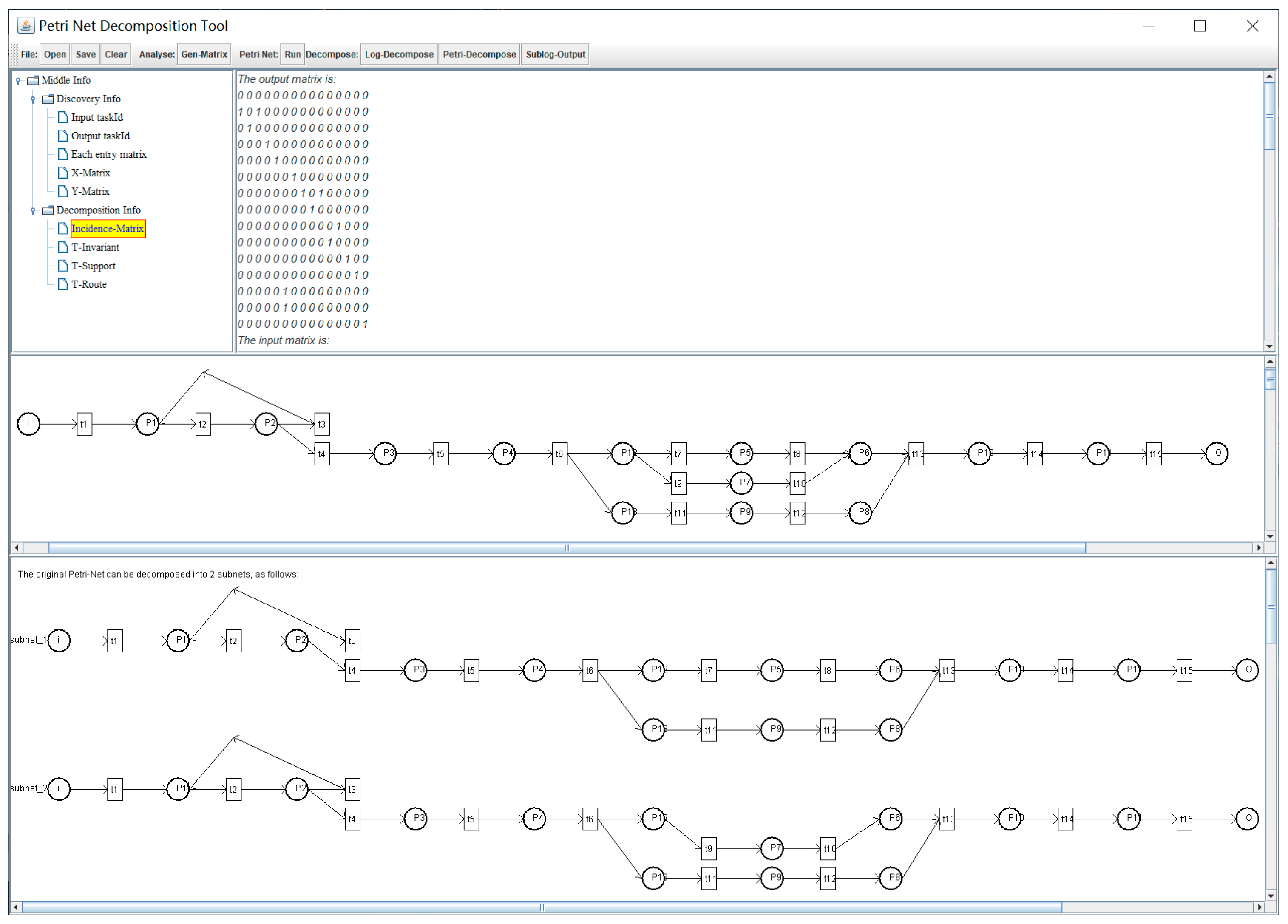
5.1. Application of Tool

We applied the Petri nets analysis tool developed in Section 4 to the software testing process of the RSA timing attack tasks. The test team performed the testing work on the workflow management system supporting the software testing process according to the software requirements specification, fed back the results for each stage test in real time, and recorded the corresponding failure interval time. During the testing process, the faults detected were classified into inherent faults and human faults, and we needed to provide the corresponding test reports and repair the faults detected in the software. With regard to different test data, we can select a more appropriate SRGM to predict the failure time in the future and then analyze the reliability degree of the system. During the process of workflow debugging (faults detection and repair), it is important to determine the key factors that affect the normal execution of the process through the application of stochastic Petri nets analysis tools to supervise the debugging process and improve the decision-making process of software testing, which is helpful for testers to perform reliability growth analysis.
The logs from the WFMS truly recorded the software testing workflow of the RSA timing attack tasks, and the Petri nets acquisition component established a structured process model by mining the log information. The original model was analyzed by the Petri nets decomposition component to generate sublogs and subnets. According to the decomposed subprocesses, the Petri nets combination component recombined the unreasonable processes of the original model and verified the differences in the testing processes between the models before and after the recombination. We followed the ADCV method to solve the problem of the BPM modeling of the software testing platform WFMS, which was beneficial to establishing a more accurate SRGM for the tested software and improving its reliability measurement results. The testing workflow for the RSA timing attack tasks is shown in Figure 12.
During the process of testing execution, when the current execution violated the principle of the testing process shown in Figure 12, the Petri nets analysis tool immediately determined the wrong process execution and suspended the token transfer to the next transition. After the process was corrected to the normal state, the token continued to be transferred to the next transition. Through the supervision of the testing process execution, we corrected the wrong execution status and improved the credibility of SRGM’s parameters. The incidence matrix and coverage graph were used to verify the legality of the process attributes in accordance with the requirements, and the results were output in the interface. Through the reachability judgment and verification of the places’ differences between the Petri nets model and the original model of business process recombination, we judged the change in requirements to verify the correctness of the tool and improve development efficiency.

5.2. Evaluation and Analysis of Tool

The workflow log information in Table 1 was generated from the second round of tests of the software related to the RSA timing attack tasks (that is, the RSA timing attack program based on the Linux platform). Eight faults were detected in the test, and the total testing time was 44.1 h. We applied the Petri nets analysis tool developed above to the second round of tests, then modeled and analyzed the software testing workflow according to the ADCV method, and finally submitted an optimized software testing workflow recombination model to the test team. Further, the test team carried out the testing work according to the recombined workflow in the next round of testing. Thirteen faults were detected in this test, and the testing time was 170.5 h (note: the third round of the test was consistent with the software requirements specification in the second round of the test). The G-O NHPP model, as a classical SRGM, has a good effect on reliability prediction and analysis. In this work, the MSE, SAE, variation, RMSPE, and R2 were adopted as assessment indexes to evaluate the prediction ability of the G-O NHPP model on the fault datasets DS2 and DS3. The assessment results are shown in Table 2.
If the value of the MSE, SAE, variation, or RMSPE is smaller, the predictive power of the model is stronger; if the value of R2 is closer to 1, the predictive power of the model is stronger. As shown in Table 2, the values of the MSE, variation, RMSPE, and R2 of the G-O NHPP model on DS3 were better than the corresponding index values on DS2; hence, the fitting power of the G-O NHPP model on DS3 was better than that on DS2, which indirectly indicated that the parameter estimation of the G-O NHPP model based on DS3 was more accurate. It can be seen that the software testing workflow recombination model provided by the ADCV method after the end of the second round of the test had certain validity, showing good results in SRGM parameter estimation and reliability prediction.

6. Conclusions

The automation and digitalization of business processes have enabled information systems to capture a large amount of log data, which can help enterprises or organizations better understand the workflow, improve the workflow, and provide operational support. By monitoring and managing business processes, we can identify process bottlenecks, recombine processes, and create the status space of process instances to explore their quality attributes. This work achieved some good results for the research into the ADCV modeling method, but there are still many things worth studying from the perspective of the practical application of software testing workflow. The Petri nets analysis tool completes the function of automatic requirement analysis for the trusted workflow management system and aims to establish a workflow model according to the methods of process acquisition, decomposition, combination, and verification, and continuously carries out the iterative cycle of BPM based on users’ requirements until the new model is accepted by process design users. In the software testing process, we apply the tool to complete the supervision of the testing process and testing data to improve the decision-making process of debugging and the quality of reliability analysis.
The ADCV method covers relevant algorithms and technologies such as process mining, process decomposition, process recombination, and process verification, but it does not involve the analysis of the process automation combination algorithm. This aspect will be further discussed in the follow-up research. In addition, it will also enrich and expand the methods in the process verification link to enhance the ability of process analysis. When applying the ADCV method to the software testing workflow, the SRGM modeling was not deeply combined with the Petri nets theory. In future work, we will continue to optimize the ADCV method to find the adverse factors that affect the SRGM parameter estimation in the software testing process and propose corresponding improvement countermeasures. Reference [41] uses the object-centered event log to predict the ongoing process in the most advanced prediction model. Its proposed model uses the rich data contained in the OCEL (object-centric event log) to enhance the latest progress of the prediction methods, which provides a new research idea for the research on the ADCV method and also provides a reference for the prediction of business process failure behavior.
Overall, this paper has conducted a preliminary investigation into the modeling problem of BPM in two ways: one is the fundamental modeling method of the original BPM based on an iterative pattern, and the other is the advanced modeling technology of the software testing workflow based on Petri Net. In the future, the combination algorithm should be optimized, as its massive combinatorial space with high dimensions has posed a strong challenge for the implementation of the ADCV method; at the same time, the enterprise software testing processes should be applied in the tool to improve its practicality on SRGM.

Author Contributions

Ideas, Q.H. and Z.M.; methodology, Q.H. and Z.M.; writing—original draft preparation, Z.M.; writing—review and editing, Q.H., Y.H., N.L., C.L., Z.S., and S.H.; software, Q.H. and Z.M.; data curation, Y.H., N.L., and C.L.; algorithm combination, Z.S.; data collation, S.H; funding acquisition, Q.H. All authors have read and agreed to the published version of the manuscript.

Funding

This research was supported by the National Natural Science Foundation of China (Grant No. 61862001) and the high-level talents (top academic talents) of North Minzu University (Grant No. 2019BGBZ07).

Data Availability Statement

Not applicable.

Acknowledgments

We are grateful for the support and help in scientific research offered by the Key Laboratory of Images & Graphics Intelligent Processing of State Ethnic Affairs Commission, North Minzu University (IGIPLab). The authors would like to thank the anonymous reviewers and editors for their suggestions.

Conflicts of Interest

The authors declare no conflict of interest.

References

  1. Han, Q.; Yang, D. Hierarchical Information Entropy System Model for TWfMS. Entropy 2018, 20, 732. [Google Scholar] [CrossRef] [PubMed]
  2. Sakr, S.; Maamar, Z.; Awad, A.; Benatallah, B.; Aalst, W. Business Process Analytics and Big Data Systems: A Roadmap to Bridge the Gap. IEEE Access 2018, 6, 77308–77320. [Google Scholar] [CrossRef]
  3. Cinque, M.; Cotroneo, D.; Pecchia, A.; Pietrantuono, R.; Russo, S. Debugging-Workflow-Aware Software Reliability Growth Analysis. Softw. Test. Verif. Reliab. 2017, 27, e1638. [Google Scholar] [CrossRef]
  4. Kaid, H.; Al-Ahmari, A.; Li, Z.; Davidrajuh, R. Intelligent Colored Token Petri Nets for Modeling, Control, and Validation of Dynamic Changes in Reconfigurable Manufacturing Systems. Processes 2020, 8, 358. [Google Scholar] [CrossRef]
  5. Cong, X.; Fanti, M.P.; Mangini, A.M.; Li, Z. Critical Observability of Discrete-Event Systems in a Petri Net Framework. IEEE Trans. Syst. Man Cybern. Syst. 2022, 52, 2789–2799. [Google Scholar] [CrossRef]
  6. Zhang, C.; Cui, G.; Liu, H.; Meng, F. Component-Based Software Reliability Process Technologies. Chin. J. Comput. 2014, 37, 2586–2612. [Google Scholar]
  7. Zhang, C.; Meng, F.; Kao, Y.; Lv, W.; Liu, H.; Wan, K.; Jiang, J. Survey of Software Reliability Growth Model. J. Softw. 2017, 28, 2402–2430. [Google Scholar]
  8. Inoue, S.; Yamada, S. Markovian Software Reliability Modeling with Change-Point. Int. J. Reliab. Qual. Saf. Eng. 2018, 25, 1850009. [Google Scholar] [CrossRef]
  9. Xu, J.; Pei, Z.; Guo, L.; Zhang, R.; Wang, F. Reliability Analysis of Cloud Service-Based Applications Through SRGM and NMSPN. J. Shanghai Jiaotong Univ. (Sci.) 2020, 25, 57–64. [Google Scholar] [CrossRef]
  10. Aalst, W.; Weijters, A.; Măruşter, L. Workflow Mining: Discovering Process Models from Event Logs. IEEE Trans. Knowl. Data Eng. 2004, 16, 1128–1142. [Google Scholar] [CrossRef]
  11. Liu, G.; Reisig, W.; Jiang, C.; Zhou, M. A Branching-Process-Based Method to Check Soundness of Workflow Systems. IEEE Access 2016, 4, 4104–4118. [Google Scholar] [CrossRef]
  12. He, Y.; Liu, G.; Xiang, D.; Sun, J.; Yan, C.; Jiang, C. Verifying the Correctness of Workflow Systems Based on Workflow Net With Data Constraints. IEEE Access 2018, 6, 11412–11423. [Google Scholar] [CrossRef]
  13. He, Y.; Liu, G.; Yan, C.; Jiang, C.; Wang, J. Locating and Controlling Unsound Transitions in Workflow Systems Based on Workflow Net With Data Constraints. IEEE Access 2018, 6, 62622–62637. [Google Scholar] [CrossRef]
  14. Han, Q. Trustworthiness Measurement Algorithm for TWfMS Based on Software Behaviour Entropy. Entropy 2018, 20, 195. [Google Scholar] [CrossRef] [PubMed]
  15. Han, Q.; Yuan, Y. Research on Trustworthiness Measurement Approaches of Component Based BPRAS. J. Commun. 2014, 35, 47–57. [Google Scholar]
  16. Gokhale, S.S. Architecture-Based Software Reliability Analysis: Overview and Limitations. IEEE Trans. Dependable Secur. Comput. 2007, 4, 32–40. [Google Scholar] [CrossRef]
  17. Martins, J.; Branco, F.; Au-Yong-Oliveira, M.; Gonçalves, R.; Moreira, F. Higher Education Students Perspective on Education Management Information Systems: An Initial Success Model Proposal. Int. J. Technol. Hum. Interact. 2019, 15, 1–10. [Google Scholar] [CrossRef]
  18. Rivest, R.L.; Shamir, A.; Adleman, L.M. A method for obtaining digital signatures and public-key cryptosystems. Commun. ACM 1978, 21, 120–126. [Google Scholar] [CrossRef]
  19. Kocher, P.C. Timing Attacks on Implementations of Diffie-Hellman, RSA, DSS, and Other Systems. In Proceedings of the 16th Annual International Cryptology Conference on Advances in Cryptology, Santa Barbara, CA, USA, 18–22 August 1996; pp. 104–113. [Google Scholar]
  20. Pei, J.; Wen, L.; Yang, H.; Wang, J.; Ye, X. Estimating Global Completeness of Event Logs: A Comparative Study. IEEE Trans. Serv. Comput. 2021, 14, 441–457. [Google Scholar] [CrossRef]
  21. Martin, N.; Solti, A.; Mendling, J.; Depaire, B.; An, C. Mining Batch Activation Rules from Event Logs. IEEE Trans. Serv. Comput. 2021, 14, 1908–1919. [Google Scholar] [CrossRef]
  22. Pourbafrani, M.; Aalst, W. Discovering System Dynamics Simulation Models Using Process Mining. IEEE Access 2022, 10, 78527–78547. [Google Scholar] [CrossRef]
  23. Rogge-Solti, A.; Senderovich, A.; Weidlich, M.; Mendling, J.; Gal, A. In Log and Model We Trust? A Generalized Conformance Checking Framework. Lect. Notes Comput. Sci. 2016, 9850, 179–196. [Google Scholar]
  24. Matthias, G.; Simon, H.; Jörg, L.; Guido, W. BPMN 2.0: The State of Support and Implementation. Future Gener. Comput. Syst. 2018, 80, 250–262. [Google Scholar]
  25. Lanouar, L.; Rekik, M.; Bouchaala, O.; Krichen, L. An Optimal Power Supervising Strategy for A Smart Home Assessed Based on BPMN Framework. In Proceedings of the 2022 IEEE 21st international Ccnference on Sciences and Techniques of Automatic Control and Computer Engineering (STA), Sousse, Tunisia, 19–21 December 2022; pp. 406–411. [Google Scholar]
  26. Al-Ali, H.; Cuzzocrea, A.; Damiani, E.; Mizouni, R.; Tello, G. A Composite Machine-Learning-Based Framework for Supporting Low-Level Event Logs to High-Level Business Process Model Activities Mappings Enhanced by Flexible BPMN Model Translation. Soft Comput. 2020, 24, 7557–7578. [Google Scholar] [CrossRef]
  27. Li, N.; Han, Q.; Zhang, Y.; Li, C.; He, Y.; Liu, H.; Mao, Z. Standardization Workflow Technology of Software Testing Processes and its Application to SRGM on RSA Timing Attack Tasks. IEEE Access 2022, 10, 82540–82559. [Google Scholar] [CrossRef]
  28. ISO/IEC/IEEE 29119-2:2021(E); ISO/IEC/IEEE International Standard-Software and Systems Engineering-Software Testing—Part 2: Test Processes. IEEE: New York, NY, USA, 28 October 2021; pp. 1–64. [CrossRef]
  29. Tao, J.; Wang, J.; Wen, L.; Zou, G. Computing Refined Ordering Relations with Uncertainty for Acyclic Process Models. IEEE Trans. Serv. Comput. 2014, 7, 415–426. [Google Scholar]
  30. Kalenkova, A.; Aalst, W.; Lomazova, I.; Rubin, V. Process Mining Using BPMN: Relating Event Logs and Process Models. Softw. Syst. Model. 2017, 16, 1019–1048. [Google Scholar] [CrossRef]
  31. Pegoraro, M.; Uysal, M.; Aalst, W. Efficient Time and Space Representation of Uncertain Event Data. Algorithms 2020, 13, 285. [Google Scholar] [CrossRef]
  32. Zhang, C.; Liu, H.; Bai, R.; Wang, K.; Wang, J.; Lv, W.; Meng, F. Review on Fault Detection Rate in Reliability Model. J. Softw. 2020, 31, 2802–2825. [Google Scholar]
  33. Lee, D.; Chang, I.; Pham, H. Software Reliability Model with Dependent Failures and SPRT. Mathematics 2020, 8, 1366. [Google Scholar] [CrossRef]
  34. Tripathi, M.; Singh, L.K.; Singh, S.; Singh, P. A Comparative Study on Reliability Analysis Methods for Safety Critical Systems Using Petri-Nets and Dynamic Flowgraph Methodology: A Case Study of Nuclear Power Plant. IEEE Trans. Reliab. 2022, 71, 564–578. [Google Scholar] [CrossRef]
  35. Goel, A.L.; Okumoto, K. Time-Dependent Error-Detection Rate Model for Software Reliability and Other Performance Measures. IEEE Trans. Reliab. 1979, R-28, 206–211. [Google Scholar] [CrossRef]
  36. Nagaraj, V. Software Reliability Assessment: Modeling and Algorithms. In Proceedings of the 2018 IEEE International Symposium on Software Reliability Engineering Workshops (ISSREW), Memphis, TN, USA, 15–18 October 2018; pp. 166–169. [Google Scholar]
  37. Li, S.; Dohi, T.; Okamura, H. A Comprehensive Evaluation for Burr-Type NHPP-based Software Reliability Models. In Proceedings of the 2021 8th International Conference on Dependable Systems and Their Applications (DSA), Yinchuan, China, 5–6 August 2021; pp. 1–11. [Google Scholar]
  38. Garg, R.; Raheja, S.; Garg, R.K. Decision Support System for Optimal Selection of Software Reliability Growth Models Using a Hybrid Approach. IEEE Trans. Reliab. 2022, 71, 149–161. [Google Scholar] [CrossRef]
  39. Song, L.; Minku, L.L. A Procedure to Continuously Evaluate Predictive Performance of Just-In-Time Software Defect Prediction Models during Software Development. IEEE Trans. Softw. Eng. 2023, 49, 646–666. [Google Scholar] [CrossRef]
  40. Jagtap, M.; Katragadda, P.; Satelkar, P. Software Reliability: Development of Software Defect Prediction Models Using Advanced Techniques. In Proceedings of the 2022 Annual Reliability and Maintainability Symposium (RAMS), Tucson, AZ, USA, 24–27 January 2022; pp. 1–7. [Google Scholar]
  41. Galanti, R.; Leoni, M.D.; Navarin, N.; Marazzi, A. Object-centric Process Predictive Analytics. Expert Syst. Appl. 2023, 213, 119173. [Google Scholar] [CrossRef]
Figure 1. Petri nets models for fundamental workflow modes. (a) sequential mode; (b) parallel split mode; (c) synchronous mode; (d) exclusive selection mode; (e) simple merge mode; (f) forced circulation modeI.
Electronics 12 04464 g001
Figure 2. Reference model for a trustworthy workflow management system (TWfMS).
Electronics 12 04464 g002
Figure 3. Compositional structure of the ADCV method.
Electronics 12 04464 g003
Figure 4. Model transformation relationship of the ADCV method.
Electronics 12 04464 g004
Figure 5. Hierarchical diagram of process mining.
Electronics 12 04464 g005
Figure 6. The situations of a > L b , b > L a , a × L b , and b × L a .
Electronics 12 04464 g006
Figure 7. GUI of Petri nets acquisition component.
Electronics 12 04464 g007
Figure 8. GUI of Petri nets decomposition component.
Electronics 12 04464 g008
Figure 9. GUI of Petri nets combination and verification components.
Electronics 12 04464 g009
Figure 10. Test monitoring and control processes mapped with the ADCV method.
Electronics 12 04464 g010
Figure 11. Modeling and evaluation process of SRGM.
Electronics 12 04464 g011
Figure 12. BPMN of the testing workflow for the RSA timing attack tasks.
Electronics 12 04464 g012
Table 1. Detailed data of event log.
CaseIdEventCaseIdEventCaseIdEventCaseIdEvent
NameStatusNameStatusNameStatusNameStatus
1T1Start1T14Start2T10Complete3T6Start
1T1Complete1T14Complete2T12Complete3T6Complete
1T2Start1T15Start2T13Start3T11Start
1T2Complete1T15Complete2T13Complete3T7Start
1T4Start2T1Start2T14Start3T11Complete
1T4Complete2T1Complete2T14Complete3T12Start
1T5Start2T2Start2T15Start3T7Complete
1T5Complete2T2Complete2T15Complete3T8Start
1T6Start2T4Start3T1Start3T8Complete
1T6Complete2T4Complete3T1Complete3T12Complete
1T11Start2T5Start3T2Start3T13Start
1T7Start2T5Complete3T2Complete3T13Complete
1T7Complete2T6Start3T3Start3T14Start
1T8Start2T6Complete3T3Complete3T14Complete
1T11Complete2T11Start3T2Start3T15Start
1T12Start2T9Start3T2Complete3T15Complete
1T8Complete2T9Complete3T4Start4T1Start
1T12Complete2T10Start3T4Complete4T1Complete
1T13Start2T11Complete3T5Start4T2Start
1T13Complete2T12Start3T5Complete.........
Table 2. Performance indexes of business processes.
Fault Datasets/
Assessment Indexes
MSESAEVariationRMSPER2
DS20.531744.957240.605240.759950.89872
DS30.516587.748760.486690.731300.96310
Disclaimer/Publisher’s Note: The statements, opinions and data contained in all publications are solely those of the individual author(s) and contributor(s) and not of MDPI and/or the editor(s). MDPI and/or the editor(s) disclaim responsibility for any injury to people or property resulting from any ideas, methods, instructions or products referred to in the content.

