Article

ESTUGAN: Enhanced Swin Transformer with U-Net Discriminator for Remote Sensing Image Super-Resolution

School of Electronical and Information Engineering, Shenyang Aerospace University, Shenyang 110136, China
*
Author to whom correspondence should be addressed.
Electronics 2023, 12(20), 4235; https://doi.org/10.3390/electronics12204235
Submission received: 28 August 2023 / Revised: 30 September 2023 / Accepted: 11 October 2023 / Published: 13 October 2023
(This article belongs to the Special Issue Deep Learning in Computer Vision and Image Processing)

Abstract

:
Remote sensing image super-resolution (SR) is a practical research topic with broad applications. However, the mainstream algorithms for this task suffer from limitations. CNN-based algorithms face difficulties in modeling long-term dependencies, while generative adversarial networks (GANs) are prone to producing artifacts, making it difficult to reconstruct high-quality, detailed images. To address these challenges, we propose ESTUGAN for remote sensing image SR. On the one hand, ESTUGAN adopts the Swin Transformer as the network backbone and upgrades it to fully mobilize input information for global interaction, achieving impressive performance with fewer parameters. On the other hand, we employ a U-Net discriminator with the region-aware learning strategy for assisted supervision. The U-shaped design enables us to obtain structural information at each hierarchy and provides dense pixel-by-pixel feedback on the predicted images. Combined with the region-aware learning strategy, our U-Net discriminator can perform adversarial learning only for texture-rich regions, effectively suppressing artifacts. To achieve flexible supervision for the estimation, we employ the Best-buddy loss. And we also add the Back-projection loss as a constraint for the faithful reconstruction of the high-resolution image distribution. Extensive experiments demonstrate the superior perceptual quality and reliability of our proposed ESTUGAN in reconstructing remote sensing images.

1. Introduction

The rapid development of modern aerospace technology has put remote sensing imagery into wider use in the remote sensing field. Remote sensing images are essential for applications such as target detection and tracking. However, obtaining high-resolution (HR) remote sensing images can be challenging due to technical limitations and cost constraints. Image super-resolution (SR) is a promising option and a heated technology in recent years that provides critical research significance. In recent years, deep learning-based methods for single image super-resolution (SISR) have made remarkable achievements. Since the proposal of the SRCNN [1] by Dong et al. in 2014, CNN-based methods have significantly advanced the field of SR. Scholars have continuously improved network architecture and proposed elaborate structures [2,3,4], such as residual learning, dense connectivity, Laplace pyramid, and so on. RCAN [5] has achieved another pinnacle of peak signal-to-noise ratio (PSNR) by adding the channel attention module to the CNN-based architecture. However, CNN-based methods face an unavoidable obstacle when it comes to SR. Due to the design of the convolutional layer, convolution kernels interact with the image in a content-independent process. It is illogical to use the same convolutional kernel to reconstruct different areas of the image. The transformer architecture [6,7,8,9] stands out in this case, employing the self-attention mechanism for global interaction and achieving significant performance in several visual tasks. However, due to the quadratic complexity of processing images, transformer-based models tend to generate a large number of parameters and are computationally intensive. The Swin Transformer [10] was created to combine the advantages of transformer- and CNN-based models, not only establishing long-term dependencies between images, but also processing large-sized images through a local attention mechanism. SwinIR [11] firstly applies the Swin Transformer to the field of SISR; it achieves the optimal PSNR with fewer parameters and is an enormous prospect. HAT [12] activates more input signals by concatenating the channel attention mechanism in the Swin Transformer layer and proposes the overlapping cross-window attention mechanism to optimize cross-window information interaction.
While the methods mentioned above have achieved high PSNR scores, they can produce ambiguous results. This is because they often use MSE or MAE for the one-to-one supervision of a single low-resolution (LR) image corresponding to a single high-resolution (HR) image, which can lead to pixel averaging and overly smooth and blurred outcomes. Remote sensing images are mainly used in the fields of object detection as well as geologic analysis, and we believe that the over-smoothed and blurred results generated by these networks will have a negative impact on some of the categories. To obtain more realistic images, researchers have employed Generative Adversarial Networks (GANs) to recover images with rich texture details [13,14,15,16]. Although these methods have made considerable progress, further research is necessary due to their difficulty in training and tendency to produce artifacts. An alternative approach proposed by [17] is the Best-buddy loss, which breaks the strict mapping between LR and HR set by MSE or MAE. This approach allows multiple patches close to ground truth to supervise SR, reducing the difficulty of network training while improving the perceptual quality of reconstructed images.
The learning-based approaches mentioned above offer a new development direction for the remote sensing image SR task. LGCNet [18] is the first CNN-based SR model for remote sensing images that outperforms traditional methods and verifies the effectiveness of deep learning methods. Jiang et al. [19] propose an edge enhancement network based on a GAN to enhance the edge by learning noise masks. Some algorithms [20,21,22,23,24,25,26] have achieved considerable success by adding elaborate structural designs or various attention mechanisms to CNN. Currently, learning-based methods in remote sensing image SR are developing rapidly and have achieved remarkable progress, but the challenges are still significant.
The selection of a reconstruction network better suited to the characteristics of remote sensing images is a challenging problem, because remote sensing images are characterized by a large spatial span, complex texture structure, and few pixels covered by objects, which undoubtedly produce further difficulties to reconstruction tasks [27]. To faithfully restore high-resolution images, we adopt the Swin Transformer as the backbone, which can realize long-term dependency modeling with shift windows and exploit the internal self-similarity within remote sensing images. Specifically, we adopt the Residual Hybrid Attention Group (RHAG) proposed by HAT [12] and refine its network design to obtain significant performance with fewer parameters, which is named the Enhanced Swin Transformer Network (ESTN).
However, simply utilizing a more powerful reconstruction network will not completely achieve satisfactory results in the remote sensing image SR task. This is because objects in remote sensing images cover fewer pixels, and a ship may be represented by only several pixels. Employing PSNR-based methods is vulnerable to blurred results, while GANs offer a decent solution. In addition, remote sensing images contain more diverse texture features and different regions with distinct texture differences [27]. We discovered that regions with different texture complexity in remote sensing images should not adopt the same supervision strategy. Adversarial learning should be performed for texture-rich regions to facilitate the reconstruction of fine details. However, for the smooth region, the PSNR-based method is sufficient to recover satisfactory results. Instead, feeding such regions into the discriminator may lead to uncomfortable artifacts. Existing methods do not take this concern into account. To resolve the above problems, we propose the U-Net discriminator with the region-aware learning strategy. On the one hand, the U-shaped network design allows the discriminator to fully integrate the structural information at each hierarchy level and finally obtain pixel-by-pixel feedback. On the other hand, it can divide the areas according to texture complexity, and only the detailed regions are fed into the discriminator, forcing the discriminator to focus on distinguishing complex areas and greatly suppressing artifacts. Accordingly, our discriminator can effectively assist the ESTN in predicting realistic and highly detailed images.
To further improve the perceptual quality, we also introduce the Best-buddy (BB) loss [17] and Back-projection (BP) loss to break the rigid mapping from the LR space to the HR space. This reduces the training difficulty and contributes to the recovery of realistic texture details.
Overall, the main contributions of our work are as follows:
(1)
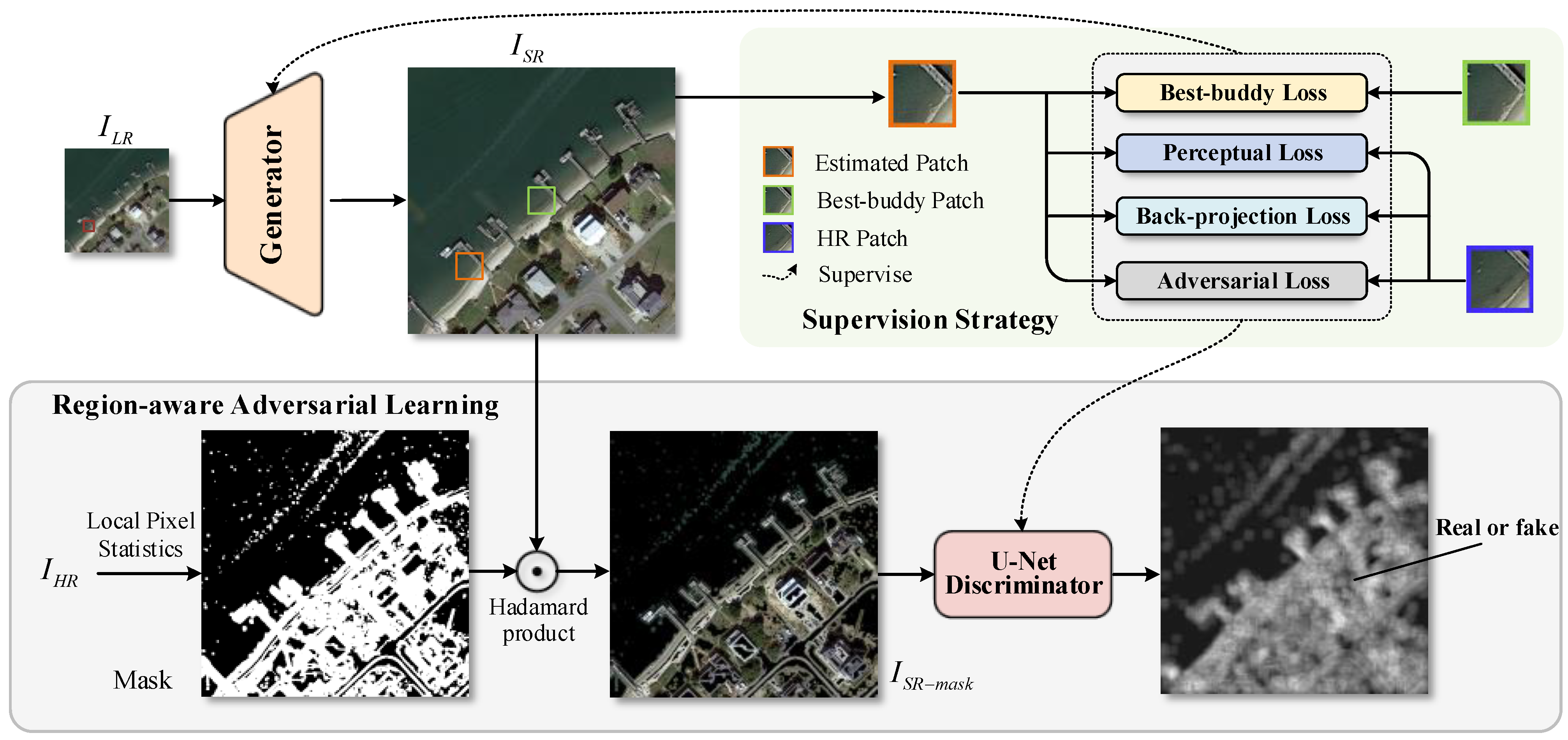
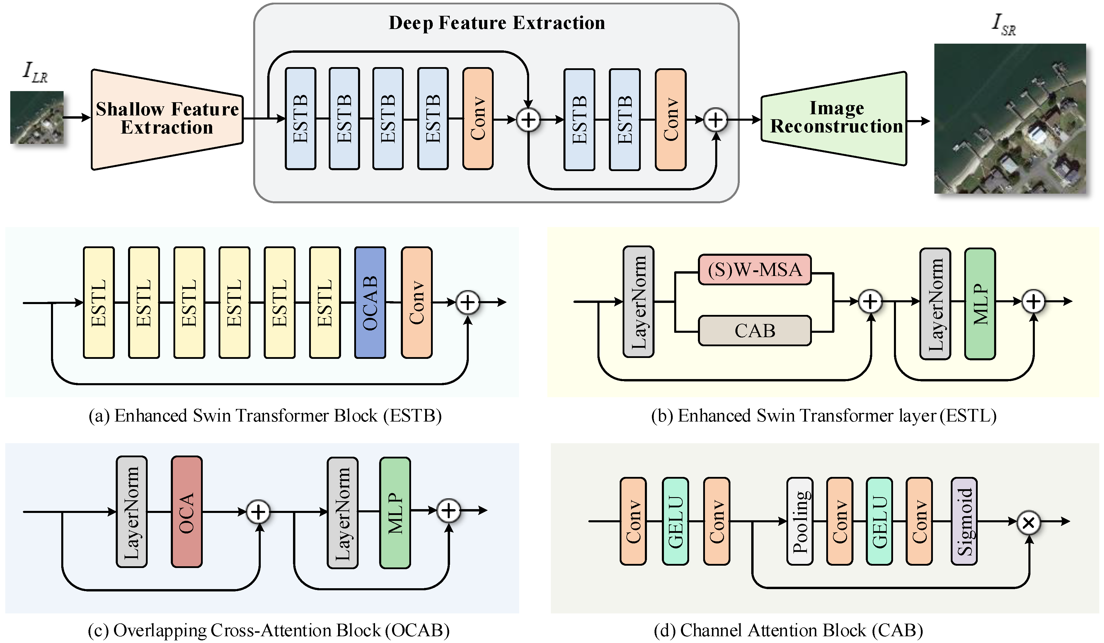
We propose a promising framework, ESTUGAN, which adopts the Enhanced Swin Transformer as the generator backbone and a U-Net discriminator. The Enhanced Swin Transformer is capable of mobilizing more input information to model local content, benefiting from united channel attention and self-attention. In addition, it employs an overlapping cross-attention mechanism to further aggregate cross-window information with stronger representational capabilities. Extensive experiments demonstrate that our proposed network outperforms other methods when targeting remote sensing image SR.
(2)
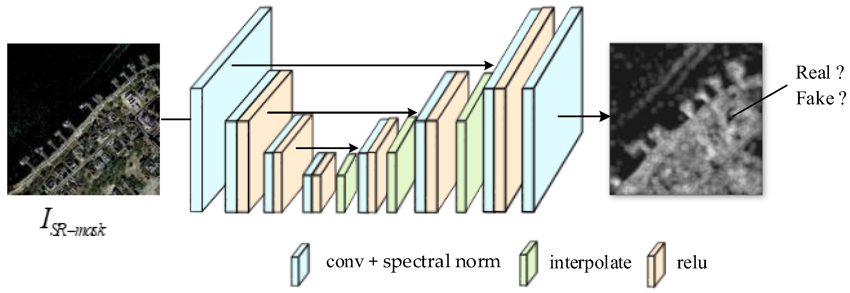
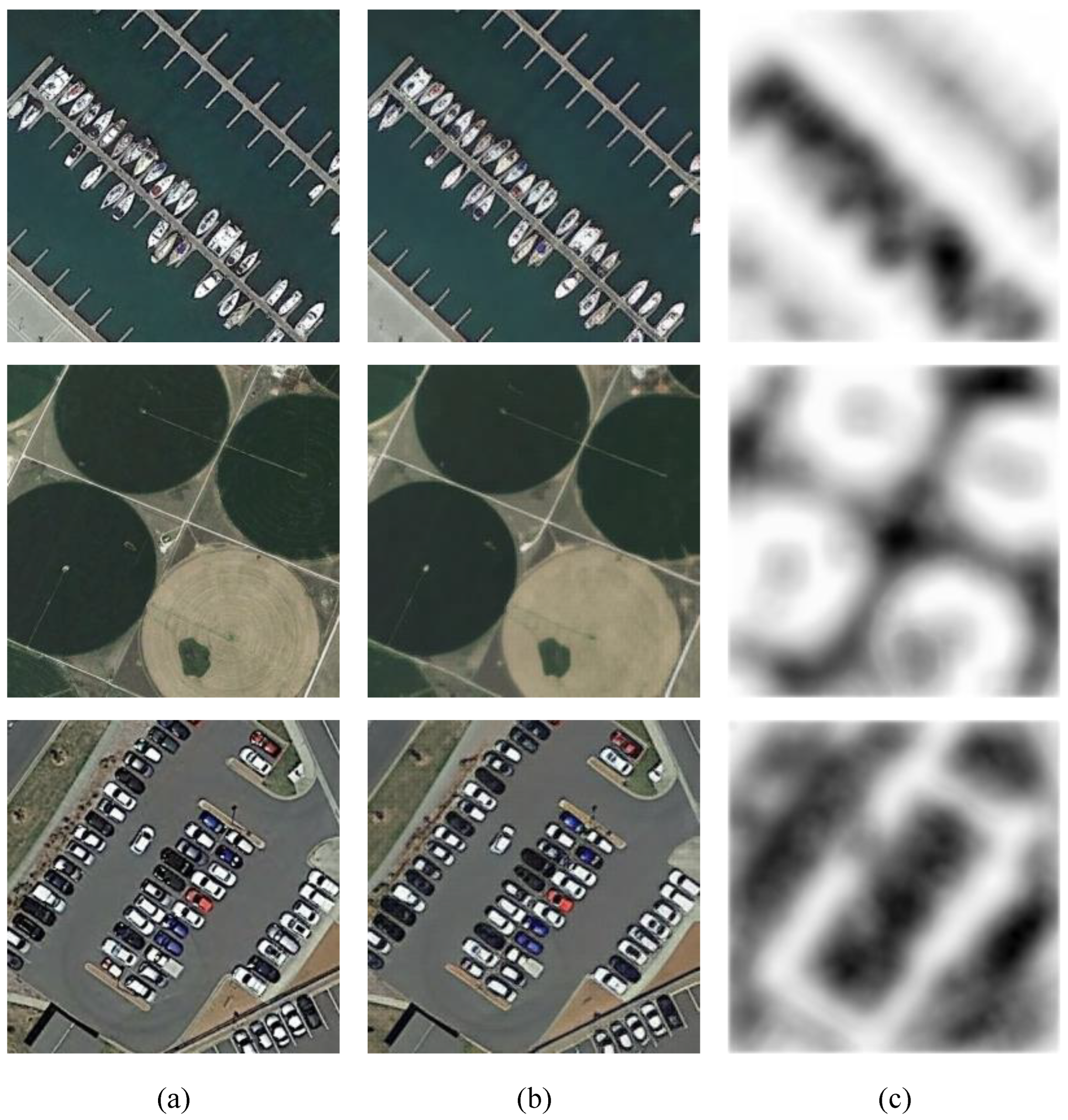
We propose a U-Net discriminator with the region-aware learning strategy to reconstruct highly detailed remote sensing images. The region-aware learning strategy can effectively suppress artifacts by masking flat regions and feeding only texture-rich regions to the discriminator for adversarial training. Moreover, the U-shaped network is designed with jumping connections that allows for the connection of shallow detailed content with deep semantic information, providing intensive feedback for each pixel’s authenticity.
(3)
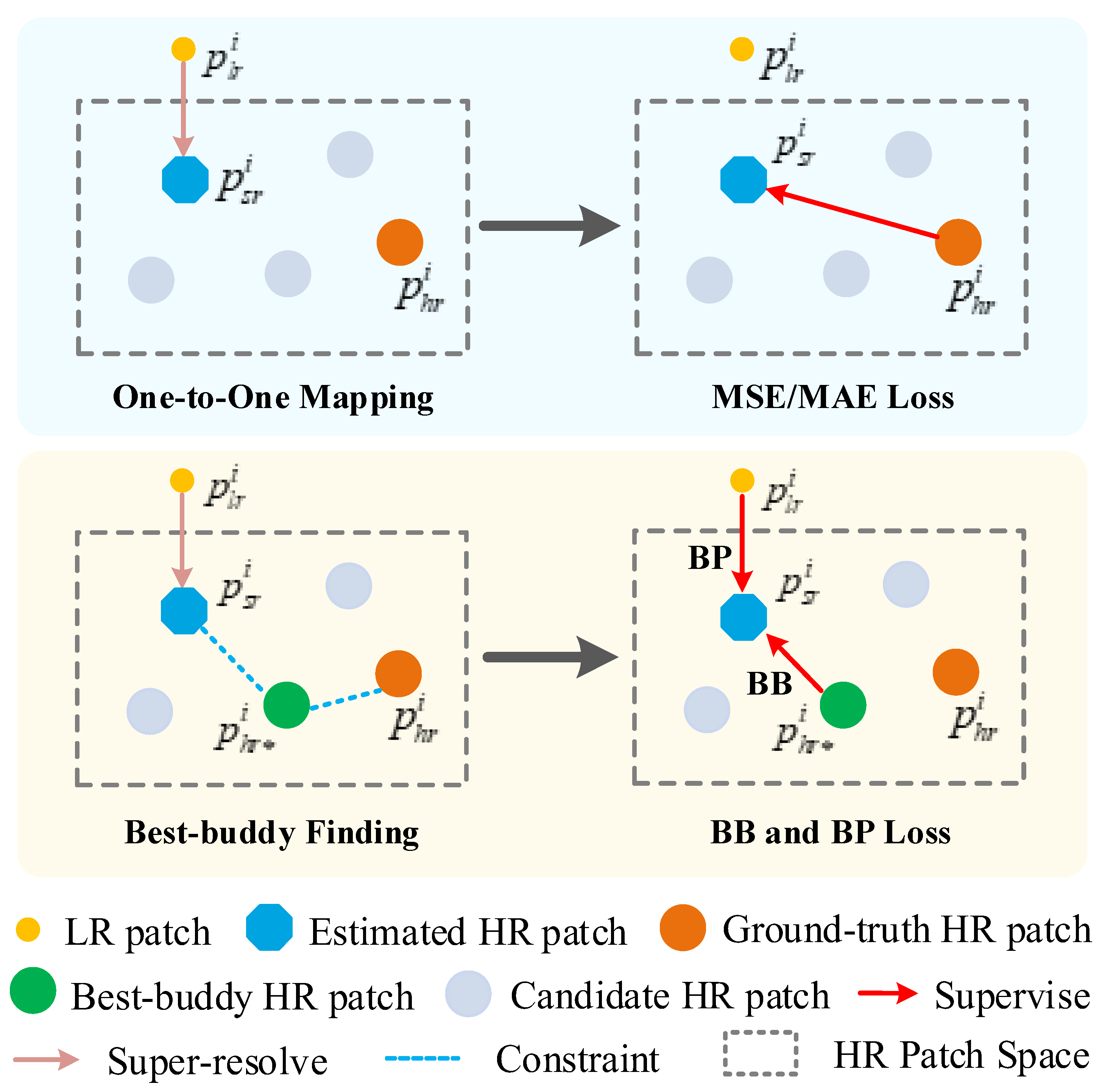
The BB loss and BP loss are employed to further enhance the visual quality of the image. Multiple supervised signals that are similar to the ground truth are utilized to flexibly guide the image reconstruction; this reduces the training difficulty and helps to generate high-frequency information.

2. Related Works

The following contents list some aspects of the previously proposed methodology related to our proposed ESTUGAN:

2.1. Swin Transformer

The Swin Transformer [10] is a universal backbone for vision tasks and represents one of the first hierarchical vision transformers. Due to its excellent performance and parallelization accessibility, it has become the state-of-the-art technology for various vision tasks such as target detection and image segmentation. The core idea of the Swin Transformer is to compute self-attention within a non-overlapping movable window, which makes the model computation linear with respect to the feature map resolution, and greatly compresses the cost of self-attention. SwinIR introduces the Swin Transformer to image SR for the first time, further refreshing the state of the art of SR tasks. However, there is still substantial room for improvement in the Swin Transformer. The window attention mechanism [28,29,30] has limitations, and the exchange of information across windows and the shallow message mobilization both require further optimization.

2.2. Generative Adversarial Network

Nowadays, GANs have been widely explored and have achieved remarkable achievements in various image processing domains such as style migration, super resolution, image complementation, and denoising tasks [31,32,33]. This approach is mainly inspired by the idea of competition in game theory, which is applied to deep learning by constructing two deep learning models: a generative network G (generator) and a discriminator network D (discriminator). The two models are then continuously played against each other to make G generate realistic images, while D has the powerful ability to determine the image authenticity. To reconstruct images with high perceptual quality, SRGAN introduces a discriminator that guides the generator to recover the fine texture information by adversarial loss. ESRGAN [15] proposes Residual-in-Residual Dense Blocks (RRDB) to build the network and invokes the relativistic GAN to make discriminators predict relative truthfulness, winning first prize in the PIRM 2018-SR Challenge. These approaches have been widely adopted as the mainstream of perception-based image SR algorithms.

2.3. Loss Function on Deep Learning

It is obvious that SISR is inherently an ill-posed problem, where a LR image often corresponds to multiple HR images. Proper guidance of the model to find the region in the latent space closest to the real HR image is the key to the SR problem. Therefore, a suitable loss function becomes particularly relevant. In existing studies, most algorithms adopt MAE/MSE loss to make the SR image approximate to the ground truth pixel by pixel. This pixel-level loss is beneficial to upgrade the PSNR but is detrimental to the reconstruction of texture details [34]. To solve this problem, perceptual loss [35] is proposed to compute the similarity of deep features to enhance the perceptual quality. Fuoli et al. [36] propose Fourier spatial loss to facilitate the recovery of lost high frequency information. Benefiting from perceptual loss and adversarial loss, SRGAN [13,14] and ESRGAN [15] recover photo-realistic outcomes, but they face the possibility of annoying artifacts. Liang et al. introduce the Local Discriminant Learning (LDL) strategy [37] that explicitly penalizes artifacts without sacrificing real details, alleviating the artifact problem partly. Li et al. suggest the Best-buddy loss [17] to address the above problems. The estimated patches are enabled to seek optimal supervision dynamically during training, contributing to the production of more reasonable details.

2.4. Deep Learning Based SISR for Remote Sensing Images

In recent years, deep learning based SISR has become mainstream due to the powerful extraction capabilities of deep neural networks. And these approaches also lead to the development and advancement of remote sensing image SR algorithms. The CNN-based SISR was widely adopted by scholars in the early days; they retrained the network on remote sensing images and designed elaborate network architectures for feature extraction. LGCNet [18] learns hierarchical representations of remote sensing images by constructing a “multifork” structure. DDRN [38] proposes ultra-dense residual blocks to construct a simple but effective recursive network. Similarly, many refined structural designs have been applied to the network with impressive achievements. However, the convolutional kernel interacts with the image in a content-independent manner, which limits the reconstruction of texture details. Some works enhance the expressive power of the model by adding various attentional mechanisms, such as MHAN [39] and SMSR [40]. But these approaches tend to be computationally intensive and still have long-term dependency modeling difficulties. In addition, the above method adopts the learning strategy which maximizes the PSNR and encourages the model to find the pixel mean, leading to blurred results. Regarding this topic, several related works have made promising progress. On the one hand, adversarial learning strategies have been employed by some works, such as SRGAN and ESRGAN, in order to reconstruct photo-realistic images. MA-GAN [27] and SRAGAN [41] combined a GAN with attention mechanisms to upgrade the visual quality of remote sensing images. On the other hand, some loss functions [35,36,37] have been proposed to motivate the generation of high-frequency content. However, these solutions are still not perfect, since problems remain, like the difficulty of GAN training and the potential for artifacts. Our work is based on a GAN, which employs the Swin Transformer as the generator for long term dependency modeling, and a U-Net discriminator with the region-aware strategy to facilitate high-frequency detail generation while suppressing artifacts to a certain extent.

2.5. Image Super Resolution Quality Assessment

SR image quality assessment is an effective way to evaluate and compare SR methods, which is an important guide for model optimization and parameter selection. Subjective human assessment represents a highly reliable evaluation approach, but it tends to be time-consuming and laborious. The PSNR [42] is the most popular metric to assess the reconstruction performance by calculating only the purely mathematical difference of pixels. Wang et al. [43] simulate the human visual system and propose an evaluation scheme based on structural similarity. However, these two options sometimes differ from the human eye’s perceptual quality, leading to ambiguous predictions. In order to maintain better consistency with subjective quality evaluations, a comparison of the feature similarity between images is employed by Zhang et al. [44] to estimate the distance from the prediction to the ground truth. The SFSN model [45] aims to find a balance between structural fidelity and statistical naturalness. Then, SRIF [46] is proposed to merge deterministic fidelity and statistical fidelity into a single prediction. Thanks to the development of deep learning, Ref. [47] extracts deep features to appraise the Learned Perceptual Image Patch Similarity (LPIPS) between two images, which is more in line with the human perceptual situation. DeepSRQ [48] with deep two-stream convolutional networks provides a satisfactory solution to the problem of no-reference evaluation.

3. Methods

In this section, we first present a brief overview on the workflow of our algorithm, and then we give a detailed description for the generator, the U-Net discriminator with the region-aware learning strategy, and the loss function employed by ESTUGAN, respectively.

3.1. Overview of ESTUGAN

For recovering images with superior perceptual quality, we designed the ESTUGAN based on a GAN, which consists of the ESTN as the generator, and the U-Net discriminator. The principal framework is shown in Figure 1. Given an LR image I L R R H × W × C , an SR image I S R R r H × r W × C (r is the scale factor) can be obtained by the generator, denoted as
I S R = G ( I L R )
where G ( · ) denotes the generator. Subsequently, unlike the approach of [14], which feeds I S R directly to the discriminator, in our approach, I S R is sent to the region-aware adversarial learning stage, where we feed only regions with rich texture details to the U-Net discriminator for authenticity judgments by regional division processing. Finally, the discriminator outputs the real probability map and feeds it back to the generator, prompting the generation of real abundant details. In a GAN, the generator is urged to deceive the discriminator by creating realistic fake HR images, while the discriminator is trained to be powerful in discriminating authenticity, and both of them compete against each other to make the SR image distribution gradually approximate the real image distribution.

3.2. The Architecture of the Generator

As shown in Figure 2, we keep the high-performance architecture design of SwinIR [11], and the whole generator is composed of three modules: shallow feature extraction, deep feature extraction, and image reconstruction.
In the shallow feature extraction module, we employ a separate convolutional layer to map the input image to a high-dimensional space. It helps the visual representation to be learned better and optimized stably. The extracted shallow features can be expressed as
F 0 = H S F ( I L R )
where H S F ( · ) denotes the shallow feature extraction.
In the deep feature extraction module, we adopt a new basic block inspired by HAT [12], called Residual Hybrid Attention Group. And we rename it to Enhanced Swin Transformer Block (ESTB) for the convenience of description, the architecture of which is shown in Figure 2a. It integrates the channel attention mechanism and the overlapping cross-attention block (OCAB), which achieves an effective aggregation for cross-window information. In addition, we insert a second residual mechanism after the convolution kernel behind the fourth ESTB. Although the residual block [49] can increase the perceptual field, we find that in low-level reconstruction tasks, such as image SR, excessively long residual connections will on the contrary weaken the generation quality of the reconstructed images, because overly abstract high-dimensional features can make network learning more difficult and cause degradation in the performance of the generation network [50]. To further demonstrate the effect of the number of residual blocks and the number of connection dimensions on the network performance, we set up three different networks in the ablation study section to demonstrate the superior performance of our network. The processes can be formulated as follows:
F D F = H D F i F 0 + F 0
F D F = H D F i F D F + F D F
where H D F i · denotes the deep feature extraction module, containing i ESTB blocks and a 3 × 3 convolutional layer. In this paper, i is set to 4 in Equation (3), and in Equation (4), i is set to 2.
In the image reconstruction module, we use jump connections to aggregate deep features and shallow features and reconstruct high-resolution images with the pixel-shuffle method [51]. It can be expressed as
I S R = H R e c F D F
where H R e c · indicates reconstruction module.

3.3. U-Net Discriminator with Region-Aware Learning Strategy

As for the discriminator, inspired by [52,53], we adopt the U-Net discriminator, which essentially consists of an encoder and a decoder to be connected, as shown in Figure 3. The encoder continuously downsamples the I S R in order to obtain the global information, and finally reacts to the overall image reality. While the decoder is dedicated to the local information authenticity judgment, it keeps performing progressive upsampling operations to output the per-pixel reality with the same resolution as I S R . In addition, skip connections are applied to facilitate the information communication between the two networks, further promoting the detailed recovery. Such a structural design forces the discriminator to focus on the structural and semantic message differences between fake and genuine samples, pursuing the accuracy of the global context and local information of the reconstruction outcome.
For addressing the artifacts of the GAN-based methods [17], the region aware strategy is appended within the U-Net discriminator, as shown in Figure 1. The smooth regions and texture-rich regions of I S R are separated by the statistical local pixel distribution of I H R , and only texture-rich regions are fed into the U-Net discriminator for adversarial learning. This not only avoids the generation of artifacts in smooth areas, but also permits the discriminator to focus on regions where fine realistic details are required to be recovered, assisting the reconstruction of perceptually realistic images. Regarding the specific region-aware learning strategy, we first perform the unfold operation with kernel size k on I H R to obtain r H × r W patches Q i , j with size k 2 . The standard deviation s t d ( Q i , j ) is then calculated for each patch, and the final binary feature map M i , j is obtained by comparison with the pre-set threshold, which is denoted as
M i , j = 0 ,                 s t d   Q i , j θ   1 ,                 s t d   Q i , j > θ
where i and j denote the specific locations of patches, and the pixel values are set to 0 for flat regions and 1 for texture-rich regions in the map. Finally, I S R _ m a s k is obtained by multiplying M i , j with I S R .
In addition, we also introduce the spectral normalization regularization [54] to further secure the stability of training and suppress artifacts.

3.4. Loss Function

3.4.1. Best-Buddy Loss

Since a single LR image can correspond to multiple HR images, SISR is intrinsically an indeterminate problem. For a given HR-LR pair, the commonly adopted MSE/MAE loss tends to perform a one-to-one rigid mapping, as shown in the blue diagram of Figure 4. This overlooks the intrinsic uncertainty of SISR, resulting in reconstructed images lacking high-frequency information. In order to overcome the limitation caused by the supervision of I S R from a single I H R , we refer to [55,56,57,58,59] and adopt the BB loss. It allows diverse supervised patches p h r i to positively steer the predicted patches p s r and achieves the multiplicity of supervision, as shown in the yellow diagram of Figure 4. For p h r i , it should be as close as possible to both the predicted patches p s r and the patch p h r of I H R , which can be expressed as
p h r i = argmin p B p p h r i 2 2 + p p s r i 2 2
where · 2 expresses L 2 loss, B denotes the supervised candidate database [17] of this image, which is obtained from the three-level image pyramid expansion achieved by the bicubic downsample operation, and i denotes the number of iterations. Then, the BB loss of this patch can be expressed as
L B B ( p s r i , p h r i ) = p s r i p h r i 1
where · 1 denotes L 1 loss.

3.4.2. Adversarial Loss

Adversarial loss is employed to facilitate perceptually realistic image generation, and the adversarial loss of the generator and discriminator are respectively denoted as
L a d v _ G = L B C E ( D I S R , U r e a l )
L a d v _ D = L B C E D I H R , U r e a l + L B C E ( D I S R , U f a k e )
where L B C E ( · ) denotes binary cross entropy loss, D ( · ) denotes the output of the discriminator, which is a tensor of shape r H × r W × 1 , U r e a l and U f a k e are tensors with the same shape as D ( · ) , where all the values of U r e a l are 1 for real labels and all the values of U f a k e are 0 for fake labels.

3.4.3. Perceptual Loss

The perceptual loss is calculated utilizing the three layers, c o n v 3 4 , c o n v 4 4 , and c o n v 5 4 , of the feature maps in the pre-trained VGG19 network, which can be expressed as
L p = i = 3 5 α i c o n v i 4 I S R c o n v i 4 I H R 1  
where α i denotes the weight occupied by each layer, and α 3 = 1/8, α 4 = 1/4, and α 5 = 1/2, respectively.

3.4.4. Back-Projection Loss

The adoption of BP loss forces the LR image obtained by downsampling I S R with r times to match I L R , achieving further supervision for I S R in the low-resolution image space, which can be denoted as
L B P = b i ( I S R , r ) I L R 1
where b i ( · , r ) denotes the bicubic downsampling operation with a scale factor r.
Thus, the overall generator loss can be expressed as
L G = μ 1 L B B + μ 2 L a d v _ G + μ 3 L p + μ 4 L B P

4. Experiments and Analysis

4.1. Datasets in Experiments

To validate the effectiveness of our proposed method, we selected four public remote sensing datasets, including the NWPU-RESISC45 dataset [60], the UCMerced dataset [61], the RSCNN7 dataset [62], and the DOTA dataset [63]. These datasets all consist of numerous RGB images and are extensively adopted in the remote sensing image SR field.

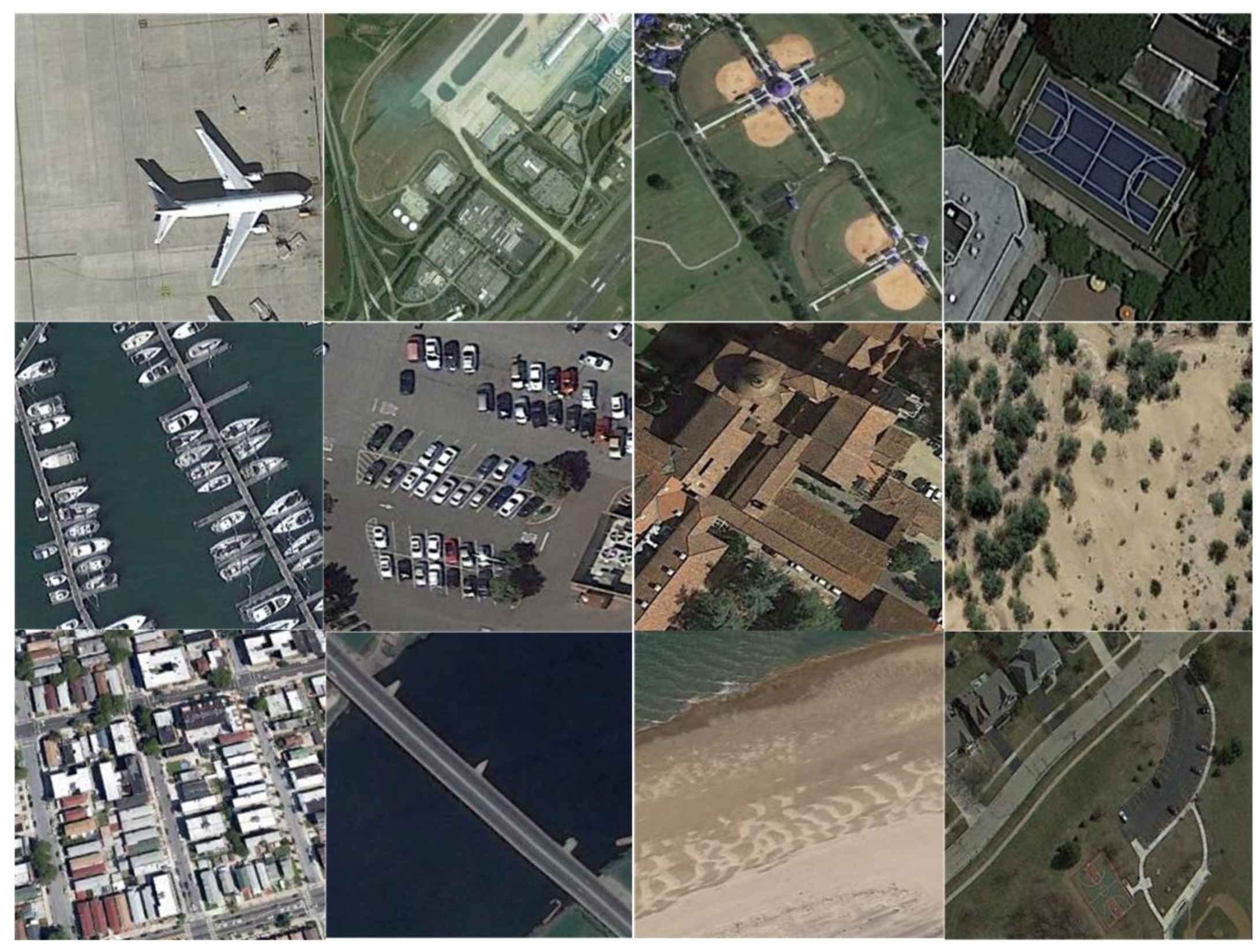
4.1.1. NWPU-RESISC45 Dataset

This dataset encompasses 45 classes of remote sensing images with high inter-class similarity and intra-class diversity. It contains a total of 31,500 images with a resolution of 256 × 256 pixels. We randomly selected 10 images in each category as the testing set for our experiments and used the rest as the training set. Some of the training set images are shown in Figure 5.

4.1.2. UCMerced Dataset

The UCMerced dataset is widely adopted for remote sensing image visual processing tasks, consisting of 21 categories, with 100 images per category. The images were captured by the remote sensing satellites of the University of California, Merced, and have a resolution of 256 × 256 pixels, covering various scenes, such as urban areas, forests, and farmlands. We randomly selected 10 images in each category as the testing set for our experiments, which can test the effectiveness of our approach and its robustness after training on the NWPU-RESISC45 dataset.

4.1.3. RSCNN7 Dataset

The RSCNN7 dataset consists of seven categories covering 2800 images and each image has 400 × 400 pixels. This dataset is sampled at different scales and takes into account weather variability and seasonal changes.

4.1.4. DOTA Dataset

The DOTA dataset consists of 2806 aerial images, each with pixel sizes ranging from 800 × 800 to 4000 × 4000, containing objects in various scales, shapes, and orientations. These images are annotated for 15 common target categories, including airplanes, ships, storage tanks, baseball fields, tennis courts, basketball courts, surface runways, harbors, bridges, large vehicles, small vehicles, helicopters, roundabouts, soccer fields, and basketball courts.

4.2. Quantitative Evaluation Metrics

In this paper, we judge the various methods using three typical image quality evaluation metrics, which are the peak signal-to-noise ratio (PSNR), the structure similarity index measure (SSIM), and the learned perceptual image patch similarity (LPIPS).

4.2.1. PSNR

The PSNR [42] is a common measure of signal reconstruction quality, and it is often defined simply by the mean squared error (MSE). For two monochrome images I and K with a size of m × n, their mean squared differences are defined as
M S E = 1 m n i = 0 m 1 j = 0 n 1 | | I i , j K ( i , j ) | | 2
Thus, the PSNR can be expressed as
P S N R = 10 l o g 10 ( M A X I 2 M S E )
where M A X I denotes the maximum pixel value in image I, and a higher PSNR value means less distortion.

4.2.2. SSIM

The SSIM [43] is also a full-reference image quality evaluation criterion, which measures image similarity in terms of brightness, contrast, and structure, respectively. It can be expressed as
S S I M = ( 2 μ x μ y + C 1 ) ( 2 σ x σ y + C 2 ) ( μ x 2 + μ y 2 + C 1 ) ( σ x 2 + σ y 2 + C 2 )
where μ x and μ y denote the mean pixel values for the two images, respectively, σ x and σ y denote the standard deviation for each image, and C 1 and C 2 are constants. The SSIM value ranges from 0 to 1, and the higher the value, the less the image distortion.

4.2.3. LPIPS

The LPIPS [47] evaluates the perceptual similarity between images according to a deep learning model, which corresponds more closely to human perception than the PSNR and SSIM do [34]. The LPIPS can be expressed as
L P I P S I H R , I S R = l 1 n l ω l ( ϕ I H R l ϕ I S R l ) 2 2
where ϕ · l indicates the feature map of the l -th convolutional layer, and n l denotes the quantity of elements in ϕ · l . denotes the product operation in the channel dimension, and ω l represents a learned weight vector. A lower value of LPIPS means that the two images are more similar in human perception.

4.3. Experimental Details

Our experiment was conducted on the NVIDIA Tesla V100 GPU. The input image size was set to 48 × 48 and the batch size was eight. We employed the bicubic operation to downsample the original high-resolution image to obtain the HR-LR training pair. The channel of our ESTN was set to sixty, and the attention heads and the window size were set to six and sixteen, respectively.
Adam was set as our optimizer and β 1 = 0.9 , β 2 = 0.999, the learning rate was 1 × 10 4 while the initial stage utilized preheating and cosine decay. k and θ were introduced in the method were are set to 11 and 0.025, respectively. As for the loss function, μ 1 , μ 3 , and μ 4 were set to 1, while μ 2 was set to 0.005 (refer to [17]).

4.4. Comparison with State-of-the-Art Methods

4.4.1. Quantitative Comparison

In our experiments, we validated the performance of our model ESTUGAN by comparing it with six deep-learning SR methods, including RCAN [5], RRDB, SwinIR [11], SRGAN [14], ESRGAN [15], and BebyGAN [17]. We selected 31050 images from the NWPU-RESISC45 dataset as the training set and 450 images as the testing set. In addition, to verify the generalizability of these models, we included 210 randomly selected images in the UCMerced dataset, 800 randomly selected images in the DOTA dataset, and all the images in the RSCNN7 dataset as additional test sets. Under the same conditions, we tested all the methods with the 4× amplification and evaluated them using the PSNR, SSIM, and LPIPS metrics.
Table 1 shows the quantitative results. It can be seen that the proposed approach achieves the most satisfactory results. In the comparison with the GAN-based methods (SRGAN, ESRGAN, and BebyGAN), ESTUGAN achieves the maximum PSNR and SSIM, and achieves the lowest LPIPS, demonstrating that it reconstructs images with optimal accuracy and perceptual quality. It is worth mentioning that ESTUGAN still maintains the best performance on three additional test sets, validating the scalability of our proposed model. In contrast, the performance of SRGAN on the DOTA dataset shows a distinct decline, reflecting the model’s shortcomings in generalizability. In the comparison with CNN-based methods (RCAN, RRDB, SwinIR), the proposed method also achieves amazing results, just slightly lower than SwinIR and higher than the other compared methods. Although it is slightly lower than SwinIR in performance, the number of parameters and FLOPs of our method are only one-fourth of those of SwinIR (illustrated in Section 4.6). The proposed method greatly saves computational resources and efficiency in the SR task for remote sensing images. The ESTN also achieves quite robust results with minimal parameters when evaluated using three additional test sets.
We also compared these methods on 45 category scenarios from the NWPU-RESISC45 dataset; as shown in Table 2, ESTUGAN outperforms the comparison methods for each scenario. Among them, the PSNR of ESTUGAN, in several scenes such as aircraft, desert, circular farmland, and industrial area, is higher than BebyGAN by over 0.3 dB, and ESTUGAN achieves the lowest LPIPS in all scenes, which means the predicted images generated by our method have the optimum visual effect. It also proves that our method can be fine-tuned for different scenes to faithfully reconstruct the actual image distribution.

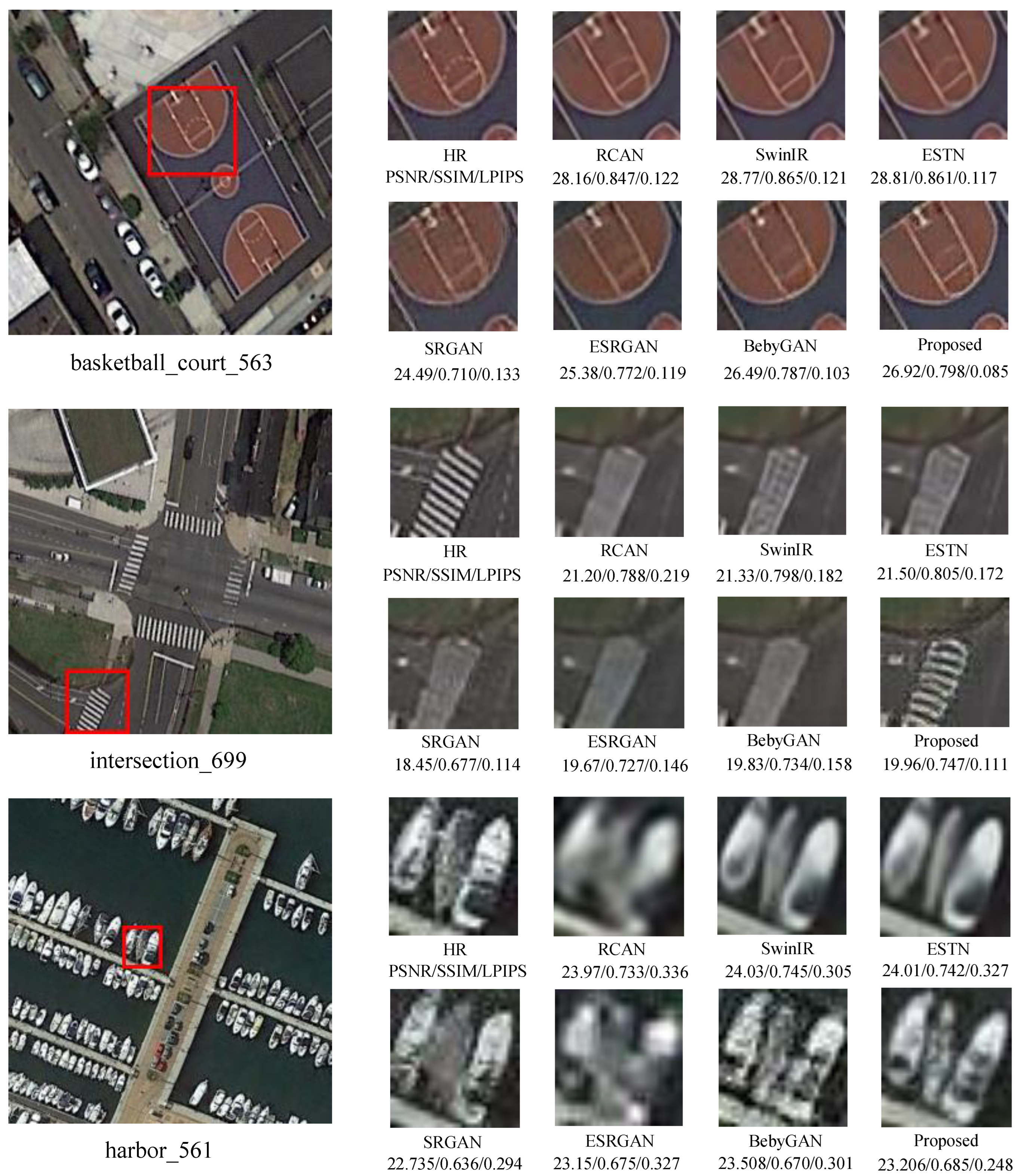
4.4.2. Qualitative Comparison
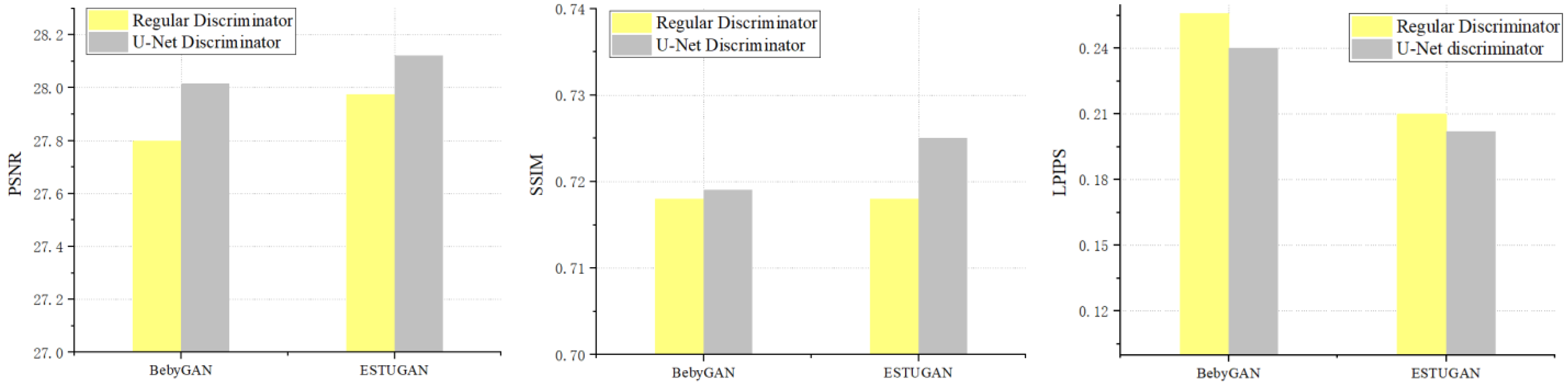
We also performed a qualitative comparison to verify the effectiveness of ESTUGAN, as shown in Figure 6. Compared to SRGAN, ESRGAN, and BebyGAN, our proposed method generates more accurate structure information and minimum artifacts, especially in the flat areas. We also reconstruct sharper and more detailed results compared to PSNR-based methods. The effectiveness of our method is well proven.

4.5. Ablation Study

We conducted ablation experiments on the test set to verify the performance of the proposed components. In order to verify the performance of the U-Net discriminator, we adopted BebyGAN and ESTUGAN as the baseline to test their performance with the U-Net discriminator and regular discriminator [14,15] respectively. As shown in Figure 7, after adopting the U-Net discriminator, the PSNR of BebyGAN improves by 0.22 dB, the LPIPS decreases by 0.012, and the SSIM increases by 0.001 dB. When replacing the U-Net discriminator with a regular discriminator in the proposed method, the PSNR drops by 0.146 dB, the LPIPS rises 0.008, and the SSIM decreases by nearly 0.01 dB, which significantly affects the reconstruction performance. This shows that the U-Net discriminator provides a more robust ability to identify authenticity. Meanwhile, we visualized the results of the discriminator determination, and the results are shown in Figure 8c, where the black pixels denote that the discriminator makes a negative judgment, while the white pixels indicate that the discriminator generates a positive judgment. Such an accurate pixel-by-pixel judgment facilitates the generator to produce better results for the LPIPS.
In addition, we also verified the effectiveness of the BB loss and the region-aware learning strategy in our approach, as shown in Table 3. Due to the elimination of the BB loss, the performance decreases on both test sets. Similarly, the PSNR, SSIM, and LPIPS deteriorate after the removal the region-aware strategy. It is noteworthy that the performance of the model without the BB loss and the region-aware learning strategy deteriorates more significantly on the UCMerced test set than on the NWPU-RESISC45 dataset. This observation underscores the potential benefits of incorporating the BB loss and the region-aware learning strategy to enhance the model generalizability.
Finally, to demonstrate the performance of our improved deep feature extraction module in the generator, we compared it with two baselines which have the same deep feature extraction module as HAT [12]. We set the number of channels to sixty and the ESTB to four (denoted as baseline1) and six (denoted as baseline2), respectively. Table 4 records the comparison results of our ESTN with two baselines on the UCMerced dataset. As can be seen from the experimental results, neither of the two baselines perform as well as our network. Although baseline2 has a deeper network structure, the effect is not better than baseline1. This proves that the residual structure will suffer performance degradation in the long-term feature extraction phase, and that cascading between residual structures will improve the performance of the remote sensing image SR task.

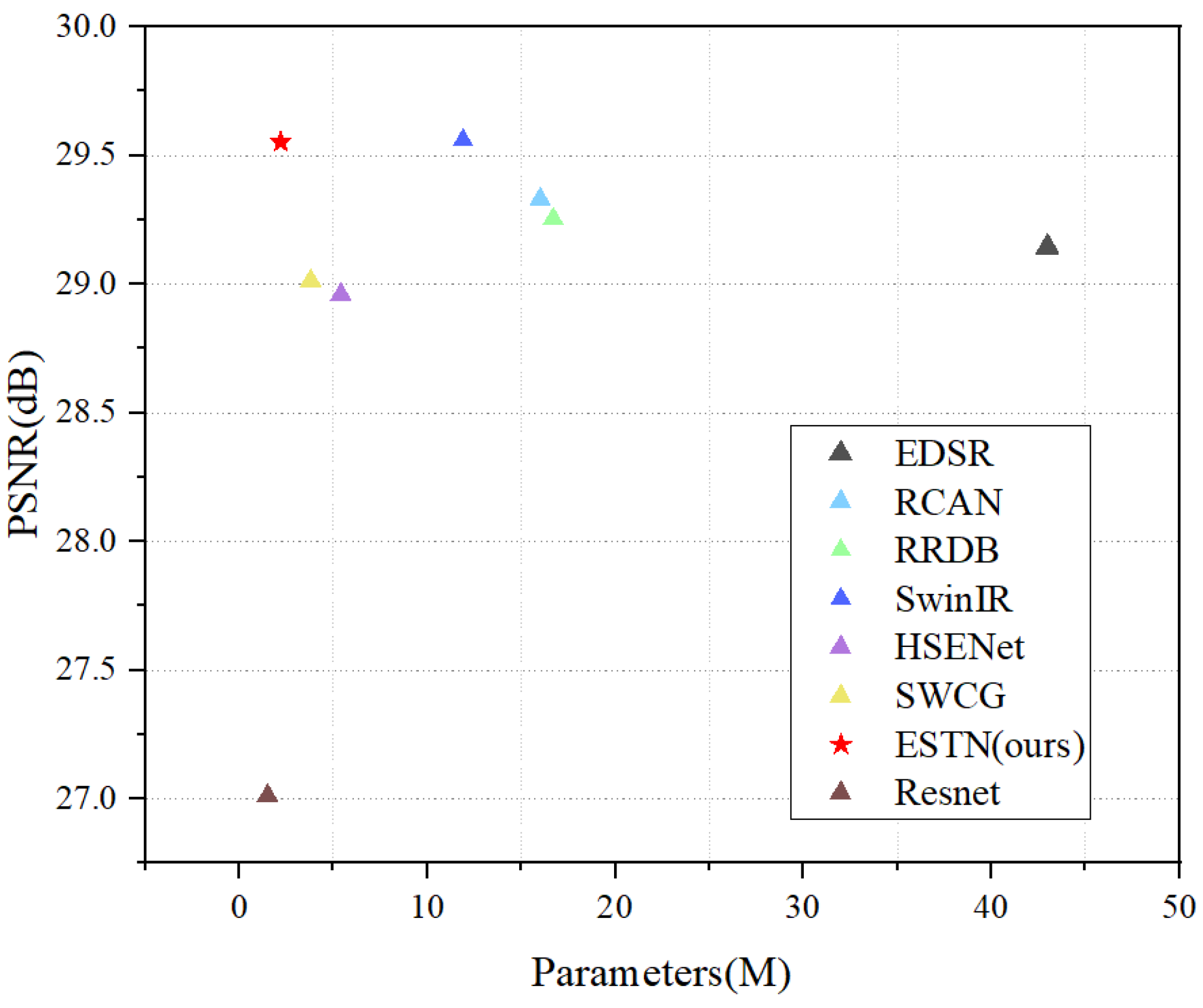
4.6. Model Complexity Analysis

Figure 9 visualizes the measurement between the parameters and the PSNR of EDSR [64], RCAN [5], RRDB [15], SwinIR [11], HSENet [24], SWCG [65], Resnet [2], and our ESTN. It can be seen that the ESTN is comparable to SwinIR in terms of performance and has an absolute advantage in the parameters, saving over nine parameters (M) compared to SwinIR. Our ESTN performs impressively in terms of the PSNR performance and the number of parameters. Table 5 comprehensively shows the parameters, FLOPs, and inference time for different methods.

5. Conclusions

In this paper, ESTUGAN was proposed for characteristics of remote sensing images. The generator was the ESTN with the backbone of the Swin Transformer, which combines the advantages of CNN- and transformer-based models, possessing a more powerful expression ability. Meanwhile, the U-Net discriminator with the region-aware learning strategy and the loss strategy that can supervise flexibility was proposed; it effectively suppressed artifacts and guided the generator to recover authentic high-frequency information. Extensive experiments proved that ESTUGAN outperforms existing methods with fewer parameters for remote sensing image SR. Specifically, we tested the performance of our model on four widely used remote sensing datasets. And for the proposed method, sufficient ablation tests were conducted to verify the validity of the components. At the same time, we also explored the network length and the performance of the image SR task to some extent; we found that just adding more functional blocks and increasing the number of parameters does not improve the overall performance, and even decreases it in some specific scenarios.
In the future, we will continue to explore the effectiveness of lightweight models for SR tasks in remote sensing images.

Author Contributions

Conceptualization, L.H.; methodology, L.H.; software, L.H. and T.P.; validation, C.Y. and L.H.; formal analysis, C.Y., L.H. and T.P.; investigation, L.H.; resources, C.Y. and L.H.; data curation, L.H.; writing-original draft preparation, L.H. and T.P.; writing-review and editing, C.Y., L.H., T.P. and Y.L.; visualization, L.H.; supervision, C.Y., Y.L. and T.L.; project administration, L.H.; funding acquisition, Y.L. All authors have read and agreed to the published version of the manuscript.

Funding

This research was supported by the Liaoning Provincial Science and Technology Department under Grant 2022JH2/101300247 and in part by the Shenyang Municipal Natural Science Foundation under Grant 23-503-6-18.

Data Availability Statement

Not applicable.

Acknowledgments

We are very grateful to the editors and reviewers for their valuable comments, to the providers of all the data used in the paper, and to the people who helped to complete this study.

Conflicts of Interest

The authors declare no conflict of interest.

References

  1. Dong, C.; Loy, C.C.; He, K.; Tang, X. Learning a Deep Convolutional Network for Image Super-Resolution. In Proceedings of the Computer Vision—ECCV 2014, Zurich, Switzerland, 6–12 September 2014; pp. 184–199. [Google Scholar]
  2. Kim, J.; Lee, J.K.; Lee, K.M. Accurate Image Super-Resolution Using Very Deep Convolutional Networks. In Proceedings of the IEEE Conference on Computer Vision and Pattern Recognition, Las Vegas, NV, USA, 26 June–1 July 2016; pp. 1646–1654. [Google Scholar]
  3. Kim, J.; Lee, J.K.; Lee, K.M. Deeply-Recursive Convolutional Network for Image Super-Resolution. In Proceedings of the IEEE Conference on Computer Vision and Pattern Recognition, Las Vegas, NV, USA, 26 June–1 July 2016; pp. 1637–1645. [Google Scholar]
  4. Lai, W.S.; Huang, J.B.; Ahuja, N.; Yang, M.H. Deep Laplacian Pyramid Networks for Fast and Accurate Super-Resolution. In Proceedings of the IEEE Conference on Computer Vision and Pattern Recognition, Honolulu, HI, USA, 26 June–21 July 2017; pp. 624–632. [Google Scholar]
  5. Zhang, Y.; Li, K.; Li, K.; Wang, L.; Zhong, B.; Fu, Y. Image Super-Resolution Using Very Deep Residual Channel Attention Networks. In Proceedings of the European Conference on Computer Vision (ECCV), Munich, Germany, 8–14 September 2018. [Google Scholar]
  6. Vaswani, A.; Shazeer, N.; Parmar, N.; Uszkoreit, J.; Jones, L.; Gomez, A.N.; Kaiser, Ł.; Polosukhin, I. Attention is All You Need. In Proceedings of the Advances in Neural Information Processing Systems 30, Long Beach, CA, USA, 4–9 December 2017. [Google Scholar]
  7. Vaswani, A.; Ramachandran, P.; Srinivas, A.; Parmar, N.; Hechtman, B.; Shlens, J. Scaling Local Self-Attention for Parameter Efficient Visual Backbones. In Proceedings of the IEEE Conference on Computer Vision and Pattern Recognition, Kuala Lumpur, Malaysia, 18–20 December 2021; pp. 1637–1645. [Google Scholar]
  8. Wang, Z.; Cun, X.; Bao, J.; Zhou, W.; Liu, J.; Li, H.U. A general u-shaped transformer for image restoration. arXiv 2021, arXiv:2106.03106. [Google Scholar]
  9. Carion, N.; Massa, F.; Synnaeve, G.; Usunier, N.; Kirillov, A.; Zagoruyko, S. End-to-end Object Detection with Transformers. In Proceedings of the European Conference on Computer Vision (ECCV), Glasgow, UK, 23–28 August 2020; pp. 213–229. [Google Scholar]
  10. Liu, Z.; Lin, Y.; Cao, Y.; Hu, H.; Wei, Y.; Zhang, Z.; Lin, S.; Guo, B. Swin Transformer: Hierarchical Vision Transformer Using Shifted Windows. In Proceedings of the IEEE/CVF International Conference on Computer Vision, Montreal, QC, Canada, 10–17 October 2021; pp. 10012–10022. [Google Scholar]
  11. Liang, J.; Cao, J.; Sun, G.; Zhang, K.; Gool, L.V.; Timofte, R. Swinir: Image Restoration Using Swin Transformer. In Proceedings of the IEEE/CVF International Conference on Computer Vision, Montreal, QC, Canada, 10–17 October 2021; pp. 1833–1844. [Google Scholar]
  12. Chen, X.; Wang, X.; Zhou, J.; Qiao, Y.; Dong, C. Activating More Pixels in Image Super-Resolution Transformer. In Proceedings of the IEEE/CVF International Conference on Computer Vision, Vancouver, BC, Canada, 18–22 June 2023; pp. 22367–22377. [Google Scholar]
  13. Goodfellow, I.; Pouget-Abadie, J.; Mirza, M.; Xu, B.; Warde-Farley, D.; Ozair, S.; Courville, A.; Bengio, Y. Generative adversarial networks. Commun. ACM 2014, 63, 139–144. [Google Scholar] [CrossRef]
  14. Ledig, C.; Theis, L.; Huszar, F.; Caballero, J.; Cunningham, A.; Acosta, A.; Aitken, A.; Tejani, A.; Totz, J.; Wang, Z.; et al. Photo-realistic Single Image Super-Resolution Using a Generative Adversarial Network. In Proceedings of the IEEE Conference on Computer Vision and Pattern Recognition, Honolulu, HI, USA, 21–26 July 2017; pp. 4681–4690. [Google Scholar]
  15. Wang, X.; Yu, K.; Wu, S.; Gu, J.; Liu, Y.; Dong, C.; Qiao, Y.; Loy, C.C. Esrgan: Enhanced Super-Resolution Generative Adversarial Networks. In Proceedings of the European Conference on Computer Vision (ECCV) Workshops, Munich, Germany, 8–14 September 2018. [Google Scholar]
  16. Zhang, W.; Liu, Y.; Dong, C.; Qiao, Y. Ranksrgan: Generative Adversarial Networks with Ranker for Image Super-Resolution. In Proceedings of the IEEE/CVF International Conference on Computer Vision, Seoul, Republic of Korea, 27 October–2 November 2019; pp. 3096–3105. [Google Scholar]
  17. Li, W.; Zhou, K.; Qi, L.; Lu, L.; Lu, J. Best-Buddy Gans for Highly Detailed Image Super-Resolution. In Proceedings of the AAAI Conference on Artificial Intelligence, Vancouver, BC, Canada, 22 February–1 March 2022; pp. 1412–1420. [Google Scholar]
  18. Lei, S.; Shi, Z.; Zou, Z. Super-resolution for remote sensing images via local–global combined network. IEEE Geosci. Remote Sens. Lett. 2017, 14, 1243–1247. [Google Scholar] [CrossRef]
  19. Jiang, K.; Wang, Z.; Yi, P.; Wang, G.; Lu, T.; Jiang, J. Edge-enhanced GAN for remote sensing image superresolution. IEEE Trans. Geosci. Remote Sens. 2019, 57, 5799–5812. [Google Scholar] [CrossRef]
  20. Pan, Z.; Ma, W.; Guo, J.; Lei, B. Super-resolution of single remote sensing image based on residual dense backprojection networks. IEEE Trans. Geosci. Remote Sens. 2019, 57, 7918–7933. [Google Scholar] [CrossRef]
  21. Ma, W.; Pan, Z.; Guo, J.; Lei, B. Achieving super-resolution remote sensing images via the wavelet transform combined with the recursive resnet. IEEE Trans. Geosci. Remote Sens. 2019, 57, 3512–3527. [Google Scholar] [CrossRef]
  22. Jiang, W.; Zhao, L.; Wang, Y.J.; Liu, W.; Liu, B.D. U-shaped attention connection network for remote-sensing image super-resolution. IEEE Geosci. Remote Sens. Lett. 2021, 19, 1–5. [Google Scholar] [CrossRef]
  23. Wu, H.; Zhang, L.; Ma, J. Remote sensing image super-resolution via saliency-guided feedback GANs. IEEE Trans. Geosci. Remote Sens. 2020, 60, 1–16. [Google Scholar] [CrossRef]
  24. Lei, S.; Shi, Z. Hybrid-scale self-similarity exploitation for remote sensing image super-resolution. IEEE Trans. Geosci. Remote Sens. 2021, 60, 1–10. [Google Scholar] [CrossRef]
  25. Liu, Z.; Feng, R.; Wang, L.; Han, W.; Zeng, T. Dual learning-based graph neural network for remote sensing image super-resolution. IEEE Trans. Geosci. Remote Sens. 2022, 60, 1–14. [Google Scholar] [CrossRef]
  26. Yu, Y.; Li, X.; Liu, F. E-DBPN: Enhanced deep back-projection networks for remote sensing scene image super-resolution. IEEE Trans. Geosci. Remote Sens. 2020, 58, 5503–5515. [Google Scholar] [CrossRef]
  27. Jia, S.; Wang, Z.; Li, Q.; Jia, X.; Xu, M. Multiattention generative adversarial network for remote sensing image super-resolution. IEEE Trans. Geosci. Remote Sens. 2022, 60, 1–15. [Google Scholar] [CrossRef]
  28. Liu, Z.; Hu, H.; Lin, Y.; Yao, Z.; Xie, Z.; Wei, Y.; Guo, B. Swin Transformer v2: Scaling up Capacity and Resolution. In Proceedings of the IEEE/CVF Conference on Computer Vision and Pattern Recognition, New Orleans, LA, USA, 19–24 June 2022; pp. 12009–12019. [Google Scholar]
  29. Choi, H.; Lee, J.; Yang, J. N-Gram in Swin Transformers for Efficient Lightweight Image Super-Resolution. In Proceedings of the IEEE/CVF International Conference on Computer Vision, Vancouver, BC, Canada, 18–22 June 2023; pp. 2071–2081. [Google Scholar]
  30. Hassani, A.; Shi, H. Dilated neighborhood attention transformer. arXiv 2022, arXiv:2209.15001. [Google Scholar]
  31. Karras, T.; Laine, S.; Aittala, M.; Hellsten, J.; Lehtinen, J.; Aila, T. Analyzing and Improving the Image Quality of Stylegan. In Proceedings of the IEEE/CVF Conference on Computer Vision and Pattern Recognition, Seattle, WA, USA, 16–20 June 2020; pp. 8110–8119. [Google Scholar]
  32. Brock, A.; Donahue, J.; Simonyan, K. Large scale GAN training for high fidelity natural image synthesis. arXiv 2018, arXiv:1809.11096. [Google Scholar]
  33. Karras, T.; Laine, S.; Aila, T. A Style-Based Generator Architecture for Generative Adversarial Networks. In Proceedings of the IEEE/CVF Conference on Computer Vision and Pattern Recognition, Long Beach, CA, USA, 16–20 June 2019; pp. 4401–4410. [Google Scholar]
  34. Yang, M.; Sowmya, A. New image quality evaluation metric for underwater video. IEEE Signal Process. Lett. 2014, 21, 1215–1219. [Google Scholar] [CrossRef]
  35. Johnson, J.; Alahi, A.; Fei-Fei, L. Perceptual Losses for Real-Time Style Transfer and Super-Resolution. In Proceedings of the European Conference on Computer Vision (ECCV), Amsterdam, The Netherlands, 11–14 October 2016; pp. 694–711. [Google Scholar]
  36. Fuoli, D.; Van Gool, L.; Timofte, R. Fourier Space Losses for Efficient Perceptual Image Super-Resolution. In Proceedings of the IEEE/CVF International Conference on Computer Vision, Montreal, QC, Canada, 10–17 October 2021; pp. 2360–2369. [Google Scholar]
  37. Liang, J.; Zeng, H.; Zhang, L. Details or Artifacts: A Locally Discriminative Learning Approach to Realistic Image Super-Resolution. In Proceedings of the IEEE/CVF Conference on Computer Vision and Pattern Recognition, New Orleans, LA, USA, 19–24 June 2022; pp. 5657–5666. [Google Scholar]
  38. Jiang, K.; Wang, Z.; Yi, P.; Jiang, J.; Xiao, J.; Yao, Y. Deep distillation recursive network for remote sensing imagery super-resolution. Remote Sens. 2018, 10, 1700. [Google Scholar] [CrossRef]
  39. Zhang, D.; Shao, J.; Li, X.; Shen, H.T. Remote sensing image super-resolution via mixed high-order attention network. IEEE Trans. Geosci. Remote Sens. 2020, 59, 5183–5196. [Google Scholar] [CrossRef]
  40. Zhang, S.; Yuan, Q.; Li, J.; Sun, J.; Zhang, X. Scene-adaptive remote sensing image super-resolution using a multiscale attention network. IEEE Trans. Geosci. Remote Sens. 2020, 58, 4764–4779. [Google Scholar] [CrossRef]
  41. Li, Y.; Mavromatis, S.; Zhang, F.; Du, Z.; Sequeira, J.; Wang, Z.; Zhao, X.; Liu, R. Single-image super-resolution for remote sensing images using a deep generative adversarial network with local and global attention mechanisms. IEEE Trans. Geosci. Remote Sens. 2021, 60, 1–24. [Google Scholar] [CrossRef]
  42. Huynh-Thu, Q.; Ghanbari, M. Scope of validity of PSNR in image/video quality assessment. Electron. Lett. 2008, 44, 800–801. [Google Scholar] [CrossRef]
  43. Wang, Z.; Bovik, A.C.; Sheikh, H.R.; Simoncelli, E.P. Image quality assessment: From error visibility to structural similarity. IEEE Trans. Image Process. 2004, 13, 600–612. [Google Scholar] [CrossRef] [PubMed]
  44. Zhang, L.; Zhang, L.; Mou, X.; Zhang, D. FSIM: A feature similarity index for image quality assessment. IEEE Trans. Image Process. 2011, 20, 2378–2386. [Google Scholar] [CrossRef]
  45. Zhou, W.; Wang, Z.; Chen, Z. Image Super-Resolution Quality Assessment: Structural Fidelity versus Statistical Naturalness. In Proceedings of the IEEE International Conference on Quality of Multimedia Experience (QoMEX), Virtual, 14–17 June 2021; pp. 61–64. [Google Scholar]
  46. Zhou, W.; Wang, Z. Quality Assessment of Image Super-Resolution: Balancing Deterministic and Statistical Fidelity. In Proceedings of the 30th ACM International Conference on Multimedia, Lisboa, Portugal, 10–14 October 2022; pp. 934–942. [Google Scholar]
  47. Zhang, R.; Isola, P.; Efros, A.A.; Shechtman, E.; Wang, O. The Unreasonable Effectiveness of Deep Features as a Perceptual Metric. In Proceedings of the IEEE Conference on Computer Vision and Pattern Recognition, Salt Lake City, UT, USA, 18–22 June 2018; pp. 586–595. [Google Scholar]
  48. Zhou, W.; Jiang, Q.; Wang, Y.; Chen, Z.; Li, W. Blind quality assessment for image superresolution using deep two-stream convolutional networks. Inf. Sci. 2020, 528, 205–218. [Google Scholar] [CrossRef]
  49. Chen, T.; Liu, H.; Ma, Z.; Shen, Q.; Cao, X.; Wang, Y. End-to-end learnt image compression via non-local attention optimization and improved context modeling. IEEE Trans. Image Process. 2021, 30, 3179–3191. [Google Scholar] [CrossRef]
  50. Zhang, Y.; Li, K.; Li, K.; Zhong, B.; Fu, Y. Residual non-local attention networks for image restoration. arXiv 2019, arXiv:1903.10082. [Google Scholar]
  51. Shi, W.; Caballero, J.; Huszár, F.; Totz, J.; Aitken, A.P.; Bishop, R.; Wang, Z. Real-Time Single Image and Video Super-Resolution Using an Efficient Sub-Pixel Convolutional Neural Network. In Proceedings of the IEEE Conference on Computer Vision and Pattern Recognition, Las Vegas, NV, USA, 26 June–1 July 2016; pp. 1874–1883. [Google Scholar]
  52. Ronneberger, O.; Fischer, P.; Brox, T. U-Net: Convolutional Networks for Biomedical Image Segmentation. In Proceedings of the Medical Image Computing and Computer-Assisted Intervention—MICCAI 2015: 18th International Conference, Munich, Germany, 5–9 October 2015; pp. 234–241. [Google Scholar]
  53. Schonfeld, E.; Schiele, B.; Khoreva, A. A U-Net Based Discriminator for Generative Adversarial Networks. In Proceedings of the IEEE/CVF Conference on Computer Vision and Pattern Recognition, Seattle, WA, USA, 13–19 June 2020; pp. 8207–8216. [Google Scholar]
  54. Miyato, T.; Kataoka, T.; Koyama, M.; Yoshida, Y. Spectral normalization for generative adversarial networks. arXiv 2018, arXiv:1802.05957. [Google Scholar]
  55. Kindermann, S.; Osher, S.; Jones, P.W. Deblurring and denoising of images by nonlocal functionals. Multiscale Model. Simul. 2005, 4, 1091–1115. [Google Scholar] [CrossRef]
  56. Protter, M.; Elad, M.; Takeda, H.; Milanfar, P. Generalizing the nonlocal-means to super-resolution reconstruction. IEEE Trans. Image Process. 2008, 18, 36–51. [Google Scholar] [CrossRef]
  57. Pan, T.; Zhang, L.; Song, Y.; Liu, Y. Hybrid Attention Compression Network with Light Graph Attention Module for Remote Sensing images. IEEE Geosci. Remote Sens. Lett. 2023, 20, 1–5. [Google Scholar] [CrossRef]
  58. Glasner, D.; Bagon, S.; Irani, M. Super-resolution from a single image. In Proceedings of the IEEE 12th International Conference on Computer Vision, Kyoto, Japan, 27 September–4 October 2009; pp. 349–356. [Google Scholar]
  59. Huang, J.B.; Singh, A.; Ahuja, N. Single Image Super-Resolution from Transformed Self-Exemplars. In Proceedings of the IEEE Conference on Computer Vision and Pattern Recognition, Boston, MA, USA, 8–12 June 2015; pp. 5197–5206. [Google Scholar]
  60. Cheng, G.; Han, J.; Lu, X. Remote sensing image scene classification: Benchmark and state of the art. Proc. IEEE 2017, 105, 1865–1883. [Google Scholar] [CrossRef]
  61. Yang, Y.; Newsam, S. Bag-of-Visual-Words and Spatial Extensions for Land-Use Classification. In Proceedings of the 18th SIGSPATIAL International Conference on Advances in Geographic Information Systems, San Jose, CA, USA, 2–5 November 2010; pp. 270–279. [Google Scholar]
  62. Zou, Q.; Ni, L.; Zhang, T.; Wang, Q. Deep learning-based feature selection for remote sensing scene classification. IEEE Geosci. Remote Sens. Lett. 2015, 12, 2321–2325. [Google Scholar] [CrossRef]
  63. Xia, G.S.; Bai, X.; Ding, J.; Zhu, Z.; Belongie, S.; Luo, J.; Datcu, M.; Pelillo, M.; Zhang, L. DOTA: A Large-Scale Dataset for Object Detection in Aerial Images. In Proceedings of the IEEE Conference on Computer Vision and Pattern Recognition, Salt Lake City, UT, USA, 18–22 June 2018; pp. 3974–3983. [Google Scholar]
  64. Lim, B.; Son, S.; Kim, H.; Nah, S.; Mu Lee, K. Enhanced Deep Residual Networks for Single Image Super-Resolution. In Proceedings of the IEEE Conference on Computer Vision and Pattern Recognition Workshops, Honolulu, HI, USA, 26 June–21 July 2017; pp. 136–144. [Google Scholar]
  65. Tu, J.; Mei, G.; Ma, Z.; Piccialli, F. SWCGAN: Generative adversarial network combining swin transformer and CNN for remote sensing image super-resolution. IEEE J. Sel. Top. Appl. Earth Obs. Remote Sens. 2022, 15, 5662–5673. [Google Scholar] [CrossRef]
Figure 1. The overview of our proposed ESTUGAN. The proposed U-Net discriminator with region-aware learning strategy focuses on adversarial learning in texture-rich regions and outputs a map for the true situation of each pixel. We use Best-buddy loss, Back-projection loss, perceptual loss, and adversarial loss to supervise the generator, and adversarial loss to guide the optimization for the discriminator.
Electronics 12 04235 g001
Figure 2. The framework of our proposed ESTN generator, which consists of three modules in total, including the deep feature extraction module, shallow feature extraction module, and image reconstruction module.
Electronics 12 04235 g002
Figure 3. The framework of our proposed U-Net discriminator.
Electronics 12 04235 g003
Figure 4. Our Best-buddy (BB) loss combined with Back-projection (BP) loss for supervision compared to MSE/MAE loss. Specifically, the blue plot represents the MAE/MSE loss, and the yellow plot represents the BB loss and BP loss we adopted. p l r i , p h r i , p s r i , and p h r i denote the LR patch, HR patch (ground truth), predicted HR patch, and Best-buddy HR patch in the current iteration, respectively.
Electronics 12 04235 g004
Figure 5. Partial images of the training set in the NWPU-RESISC45 dataset.
Electronics 12 04235 g005
Figure 6. Visualization comparison of various algorithms on the NWPU-RESISC45 dataset with a scale factor ×4.
Electronics 12 04235 g006
Figure 7. The performance of our proposed ESTUGAN and the BebyGAN on the NWPU-RESISC45 dataset when different discriminators are employed. The discriminators were measured using PSNR, SSIM, and LPIPS metrics.
Electronics 12 04235 g007
Figure 8. The visualization of the U-Net discriminator. (a) The original images in the selected dataset. (b) The generated images of the proposed generator. (c) The discrimination on the generated images.
Electronics 12 04235 g008
Figure 9. Visualization comparison of parametric quantities and PSNR of diverse approaches.
Electronics 12 04235 g009
Table 1. Qualitative comparison of PSNR, SSIM, and LPIPS in the NWPU-RESISC45, the UCMerced dataset, the RSCNN7 dataset, and the DOTA dataset at a four-time scale factor.
MethodNWPU-RESISC45UCMerced
PSNRSSIMLPIPSPSNRSSIMLPIPS
Bicubic27.610.6970.52826.960.6980.492
RCAN29.230.7720.34628.860.7760.318
RRDB29.200.7700.36228.860.7750.338
SwinIR29.420.7790.34029.170.7870.312
ESTN (ours)29.390.7770.34129.110.7850.312
SRGAN25.260.6440.23324.130.6450.258
ESRGAN26.180.7110.26325.240.7170.259
BebyGAN27.800.7180.26127.280.7240.257
ESTUGAN (ours)28.120.7250.20427.810.7390.208
MethodRSCNN7DOTA
PSNRSSIMLPIPSPSNRSSIMLPIPS
Bicubic27.990.6840.59230.890.8090.431
RCAN29.170.7440.44133.660.8680.267
RRDB29.160.7440.44933.650.8680.273
SwinIR29.330.7510.43633.980.8730.264
ESTN (ours)29.300.7490.43833.950.8720.266
SRGAN25.230.6080.28426.310.7320.272
ESRGAN26.240.6920.33128.190.8240.246
BebyGAN28.070.6980.31831.060.8290.233
ESTUGAN (ours)28.150.6990.27132.170.8290.179
Table 2. SR results for each class in the NWPU-RESISC45 dataset at a four-time scale factor.
Scene ClassBicubic
PSNR/LPIPS
RCAN
PSNR/LPIPS
SwinIR
PSNR/LPIPS
SRGAN
PSNR/LPIPS
ESRGAN
PSNR/LPIPS
BebyGAN
PSNR/LPIPS
ESTN (Ours)
PSNR/LPIPS
ESTGAN (Ours)
PSNR/LPIPS
Airplane28.57/0.43431.05/0.22931.42/0.22526.84/0.16826.15/0.20729.24/0.20731.32/0.22429.99/0.153
Airport27.83/0.55129.13/0.39429.26/0.39325.63/0.24425.90/0.28428.01/0.28729.22/0.39528.17/0.242
Baseball diamond27.69/0.52029.69/0.31429.88/0.31226.23/0.20126.81/0.22628.44/0.23829.85/0.31228.40/0.175
Basketball court26.53/0.51028.74/0.27629.06/0.26525.75/0.20526.18/0.25327.40/0.24929.01/0.26427.37/0.176
Beach30.05/0.48531.30/0.35031.36/0.34627.13/0.20526.13/0.28129.23/0.27531.36/0.34730.26/0.227
Bridge29.04/0.45031.05/0.26531.23/0.25828.18/0.16928.23/0.21229.56/0.22431.21/0.25929.81/0.166
Chaparral25.54/0.53327.14/0.32427.31/0.32720.74/0.32924.59/0.23325.82/0.24727.31/0.32425.74/0.158
Church24.49/0.56826.39/0.32126.60/0.31523.50/0.20724.43/0.26425.28/0.27626.57/0.31825.25/0.194
Circular farmland31.21/0.44833.26/0.24633.43/0.24229.99/0.15028.32/0.19731.52/0.20233.41/0.24132.12/0.153
Cloud34.81/0.36236.21/0.26736.38/0.27529.07/0.16827.92/0.15932.37/0.16436.35/0.27434.73/0.153
Commercial area25.98/0.57627.53/0.34127.67/0.33424.45/0.23925.38/0.27526.50/0.28227.66/0.33326.51/0.207
Dense residential22.43/0.66023.84/0.41124.01/0.39120.20/0.25722.56/0.28623.02/0.29424.00/0.39122.87/0.206
Desert32.17/0.47233.13/0.36133.23/0.36127.03/0.21425.05/0.28930.76/0.27033.26/0.35932.08/0.230
Forest28.47/0.65329.00/0.55329.03/0.54722.33/0.39227.79/0.35828.11/0.31929.04/0.54627.64/0.288
Freeway27.34/0.54428.79/0.35029.16/0.33325.71/0.23526.81/0.26627.78/0.26629.06/0.33527.84/0.198
Golf course29.26/0.53131.11/0.34031.20/0.34227.53/0.18828.56/0.24329.81/0.25931.20/0.34029.83/0.188
Ground track field27.22/0.52028.89/0.32729.19/0.31824.99/0.20326.55/0.23027.64/0.23929.10/0.32127.75/0.168
Harbor21.44/0.53422.91/0.30923.33/0.27320.25/0.17721.83/0.22422.14/0.22823.22/0.28122.04/0.171
Industrial area27.04/0.50928.88/0.31529.09/0.31624.77/0.19825.75/0.23727.35/0.24629.04/0.31527.77/0.188
Intersection23.44/0.58725.19/0.34025.38/0.32322.50/0.26923.19/0.30624.02/0.30825.43/0.32724.29/0.226
Island36.18/0.28337.43/0.18937.64/0.18733.43/0.12429.52/0.15832.35/0.16037.67/0.18735.94/0.124
Lake30.65/0.49531.78/0.37731.84/0.37726.27/0.26228.62/0.26530.19/0.25931.84/0.37830.65/0.233
Meadow29.36/0.67529.61/0.61029.63/0.60824.80/0.35728.43/0.48028.92/0.36629.63/0.60528.62/0.363
Medium residential27.45/0.63928.67/0.44228.77/0.43624.97/0.26726.95/0.31027.73/0.34128.74/0.43527.53/0.242
Mobile home park22.76/0.66024.62/0.40724.84/0.39521.56/0.23623.18/0.31323.69/0.34024.81/0.39323.60/0.235
Mountain29.70/0.55530.55/0.44430.60/0.44426.74/0.26827.23/0.29029.45/0.29330.60/0.44329.54/0.257
Overpass27.71/0.51529.66/0.32929.83/0.32127.18/0.19927.16/0.24728.48/0.26029.82/0.32528.61/0.188
Palace26.34/0.53328.11/0.33828.31/0.33323.38/0.25525.75/0.23726.94/0.23728.29/0.33727.03/0.185
Parking lot21.36/0.57923.08/0.32623.46/0.30120.13/0.22921.57/0.27121.93/0.27123.35/0.30122.30/0.215
Railway26.98/0.56928.37/0.37628.57/0.36625.76/0.21926.51/0.28627.42/0.28928.48/0.37227.35/0.209
Railway station25.95/0.54727.65/0.36727.93/0.36024.76/0.21225.13/0.25826.49/0.25327.91/0.36126.82/0.203
Rectangular farmland31.36/0.54232.78/0.36132.93/0.35630.50/0.21428.86/0.29631.16/0.29132.92/0.35831.72/0.241
River29.20/0.48230.98/0.30231.13/0.29727.97/0.17627.65/0.21029.53/0.21431.12/0.29829.78/0.177
Roundabout24.97/0.57226.41/0.38526.57/0.38223.75/0.24424.41/0.28325.58/0.29326.56/0.38125.51/0.226
Runway29.35/0.43733.07/0.24033.87/0.23429.01/0.17127.63/0.21630.71/0.21833.63/0.23531.95/0.157
Sea ice29.60/0.44731.38/0.30331.49/0.29822.89/0.37827.94/0.22129.65/0.22131.47/0.30230.14/0.182
Ship27.67/0.49429.58/0.29229.79/0.28126.34/0.20326.56/0.26628.25/0.26129.72/0.28628.44/0.187
Snowberg23.89/0.55025.10/0.40825.22/0.40019.42/0.38323.05/0.27224.19/0.28025.22/0.39824.06/0.225
Sparse residential26.94/0.65727.95/0.50628.08/0.50524.57/0.31926.10/0.39527.15/0.39128.04/0.50326.98/0.313
Stadium26.70/0.50628.49/0.32628.65/0.32524.49/0.22325.32/0.22827.15/0.23928.61/0.32427.44/0.183
Storage tank25.72/0.49427.94/0.28228.17/0.27824.98/0.18125.12/0.20426.80/0.21928.12/0.27726.84/0.154
Tennis court25.65/0.60127.51/0.37327.63/0.36624.22/0.22325.31/0.28126.27/0.29527.63/0.37026.33/0.207
Terrace28.79/0.47530.49/0.28730.66/0.28327.38/0.18326.73/0.24229.00/0.25630.62/0.28329.42/0.186
Thermal power station26.60/0.51128.51/0.31528.71/0.31225.13/0.21425.52/0.22227.07/0.23428.66/0.31027.46/0.186
Wetland31.14/0.51232.25/0.37032.35/0.36824.51/0.32929.62/0.26830.82/0.28432.36/0.36730.92/0.226
Mean27.61/0.52829.23/0.34629.42/0.34025.26/0.23326.18/0.26327.80/0.26129.39/0.34128.12/0.204
Standard deviation3.07/0.0763.03/0.0783.02/0.0792.87/0.0621.94/0.0552.50/0.0463.03/0.0782.94/0.044
Table 3. The comparison of ablation studies on BB loss and region aware strategies in the NWPU-RESISC45 dataset. “Ours” means our proposed ESTUGAN, “w/o BBL” and “w/o RA” indicate the model removing BB loss and the mode removing the region aware strategy.
DatasetMetricsOursw/o BBLw/o RA
NWPU-RESISC45PSNR28.1227.9527.98
SSIM0.7250.7170.719
LPIPS0.2040.2130.212
UC-MercedPSNR27.8127.4627.50
SSIM0.7390.7260.728
LPIPS0.2080.2170.215
Table 4. Comparison of using different generator frameworks on the UCMerced dataset.
Generator SettingsPSNRSSIMLPIPS
Baseline129.040.7830.311
Baseline228.600.7680.330
ESTN (ours)29.110.7850.312
Table 5. Parameters, FLOPs, and GPU runtime for various super-resolution models. GPU runtime is tested on the Tesla V100 GPU and the input size is 125 × 125.
ModelParametersFLOPsGPU Runtime
RCAN16 M233.8 G0.189 s
RRDB16.7 M257.5 G0.101 s
HSENet5.4 M73.3 G0.155 s
SwinIR11.9 M202.2 G0.288 s
ESTN (ours)2.2 M53.5 G0.165 s
Disclaimer/Publisher’s Note: The statements, opinions and data contained in all publications are solely those of the individual author(s) and contributor(s) and not of MDPI and/or the editor(s). MDPI and/or the editor(s) disclaim responsibility for any injury to people or property resulting from any ideas, methods, instructions or products referred to in the content.

