Infrared and Visible Image Fusion Based on Mask and Cross-Dynamic Fusion

Abstract

Both single infrared and visible images have respective limitations. Fusion technology has been developed to conquer these restrictions. It is designed to generate a fused image with infrared information and texture details. Most traditional fusion methods use hand-designed fusion strategies, but some are too rough and have limited fusion performance. Recently, some researchers have proposed fusion methods based on deep learning, but some early fusion networks cannot adaptively fuse images due to unreasonable design. Therefore, we propose a mask and cross-dynamic fusion-based network called MCDFN. This network adaptively preserves the salient features of infrared images and the texture details of visible images through an end-to-end fusion process. Specifically, we designed a two-stage fusion network. In the first stage, we train the autoencoder network so that the encoder and decoder learn feature extraction and reconstruction capabilities. In the second stage, the autoencoder is fixed, and we employ a fusion strategy combining mask and cross-dynamic fusion to train the entire fusion network. This strategy is conducive to the adaptive fusion of image information between infrared images and visible images in multiple dimensions. On the public TNO dataset and the RoadScene dataset, we selected nine different fusion methods to compare with our proposed method. Experimental results show that our proposed fusion method achieves good results on both datasets.

1. Introduction

Image fusion is a method of fusing two source images with different characteristics to obtain a more comprehensive and high-quality fusion image. Visible images have a variety of texture details, such as the shape and color of objects. However, due to the inherent constraints of the imaging sensor and the impact of the data capture environment, particular objects in the visible image might remain less discernible. Infrared images contain information about the thermal radiation characteristics of objects, but they lack rich texture detail. Clearly, both visible and infrared images have their limitations. Image fusion effectively addresses these challenges. The resultant images, fused from infrared and visible sources, retain the rich details of visible images and exhibit the pronounced target features of infrared images [1,2].

1.1. Technology Application

Infrared and visible image fusion technology has a variety of application scenarios in real life, including military, medical, remote sensing, etc.

In the military field [3], infrared and visible image fusion technology plays a crucial role, especially when dealing with complex backgrounds and harsh environments. It significantly improves target visibility and accuracy. For instance, in applications like drone reconnaissance and security surveillance, this fusion strategy maintains image clarity when there is ample ambient light. It captures heat source information imperceptible to conventional vision. This greatly enhances the safety and accuracy of surveillance. In low-light situations, the fusion images produced by this technology provide powerful support for night missions. It offers pilots a more comprehensive view of their surroundings, leading to better-informed flight decisions.

In the medical field [4,5,6], fusion technology can depict the temperature distribution of biological tissues more accurately. It assists doctors in more easily determining disease status and enhances the precision of surgical operations. Compared to solely relying on infrared thermal imaging for pinpointing disease sites in organisms, images from fusion technology align more closely with human intuitive perception. The technology integrates external morphology with internal details, rendering a doctor’s disease diagnosis more comprehensive.

In the remote sensing domain [7,8], this technology notably enhances land cover classification under intricate surface conditions, improving accuracy. For disaster monitoring and assessment, particularly in forest fire detection, infrared images can precisely pinpoint the fire’s origin. In contrast, visible images provide a detailed overview of the burning area. Fusion technology delves deeper into extracting crucial information about ignition sources from either infrared or visible images, offering invaluable insights for subsequent rescue efforts and fire control.

1.2. Related Work

In the field of infrared and visible image fusion, there are various technical classifications, including traditional fusion techniques and deep learning-based fusion methods [9].

Traditional fusion techniques mainly use mathematical transformations to transform source images into spatial or transformation domains, measure the activity level in these domains, and design fusion rules to achieve image fusion. Typical methods include methods based on multiscale transformations [10,11], methods based on sparse representations [12], and subspace-based methods [13,14].

The method based on multiscale transformation plays an important role in the field of infrared and visible image fusion. Its core idea is to decompose the image into sub-images of different scales and then fuse them, comprising three steps: scale decomposition, fusion strategy, and fusion reconstruction. Multiscale transformation technology helps to capture image details and global information at different scales while effectively suppressing noise and enhancing target information. Recently, various multiscale transformation techniques, such as Laplacian pyramid transform [15], discrete wavelet transform [16,17], curved wave transform [18], and multiscale pixel-level image fusion, have been successfully applied in image fusion.

The fusion method based on sparse representation aims to use an overcomplete dictionary to represent signals as linear combinations of a small number of basis vectors. First, sparse representation is used to represent the infrared and visible source images. Then, for each pixel in the sparse representation, the basis vectors from different source images are merged into a new base vector. Finally, the new basis vectors are reconstructed into a fused image according to certain rules. The fusion method for infrared and visible images, based on sparse representation technology, can effectively leverage the characteristics of both image types. It extracts useful information from both visible and infrared images and combines them to produce richer and clearer fused images.

Compared to the sparse representation-based fusion method, the subspace-based fusion method treats the visible and infrared images as two separate datasets. Then, the samples in each dataset are projected separately from the high-dimensional source image into different low-dimensional subspaces, each of which describes different local characteristics of the samples. This method allows the relationships between samples to be efficiently compared in subspace, facilitating the analysis and processing of the data.

However, traditional methods can lead to information loss during fusion, especially in subtle features such as edges, textures, and details. In addition, these methods often require manual selection and design of features, which can result in poor performance across different data and scenarios with limited generalization capabilities.

With the rapid development of deep learning technology in computer vision, many infrared and visible image fusion methods based on deep learning have emerged. In the process of infrared and visible image fusion, the deep learning method can automatically learn the features of the input data more effectively. Furthermore, it can capture the complex relationship between different band images, improving the image fusion quality and model adaptive ability, and having a more vital adaptive ability and generalization ability. Mainstream deep learning-based fusion methods are mainly divided into image fusion technology based on autoencoders (AE) [19,20]; image fusion technology based on convolution neural networks (CNN); and image fusion technology based on generative adversarial networks (GAN) [21].

AE-based image fusion technology achieves feature extraction and reconstruction through training an autoencoder. First, the autoencoder extracts features from different images. Then, it fuses this feature information based on specific rules. Finally, the fusion image is generated by a reverse reconstruction process. DenseFuse [19] is one of the best-known autoencoder-based methods. As a supervised model, it trains encoders and decoders on the MS-COCO [22] dataset. It employs a pre-trained autoencoder to decompose and reconstruct images. This approach moves away from the image decomposition method typical of traditional image fusion. Instead, it leverages the potent feature extraction capabilities of convolutional neural networks. These networks offer superior adaptability to various images compared to traditional methods. However, since DenseFuse employs only visible images during autoencoder training, it might become insensitive to certain concealed information in infrared images during feature extraction and reconstruction. This can also result in shortcomings in extracting complementary information between infrared and visible feature maps in the fusion process.

CNN-based image fusion techniques include end-to-end fusion methods [23] and fusion methods that combine CNNs with traditional methods [24]. In IFCNN [25], Zhang et al. propose an end-to-end CNN-based method that uses two convolutional layers to extract image features and then uses appropriate fusion rules for the convolution features of multiple input images, and finally performs two-layer convolution reconstruction of the fused features to obtain the final fusion image. It proposes a proportional retention loss of gradient and intensity to guide the network to directly generate fused images. In U2Fusion [26], Xu et al. propose an unsupervised end-to-end fusion network that can be applied to different types of images, automatically learning the relationships between images and implementing image fusion without the need for additional labeled data to solve different fusion problems in image fusion. Furthermore, in a fusion approach that combines CNNs with traditional methods, Liu et al. [27] use convolutional networks to generate weight maps. They then employ multiscale image decomposition and reconstruction through image pyramids to produce medical images that align more with human visual perception. Wang et al. [24] use a contrast pyramid to decompose the source images and fuse the source image in the trained CNN according to different spatial frequency bands and weighted fusion operators. However, some CNN-based fusion methods rely solely on the results of the last layer for image features, potentially resulting in the loss of valuable information from intermediate layers.

GAN-based image fusion technology relies on the adversarial game between the generator and the discriminator to estimate the probability density of the target to generate the fusion image implicitly. In FusionGAN [21], as pioneers of GAN-based image fusion, Ma et al. further enrich significant target and texture details in fused images by establishing adversarial generative rules between fused images and infrared (visible) images. However, a single discriminator can cause patterns in the fused image to be biased towards either visible or infrared images, which inevitably forces the fused image to be similar to something of little interest in the infrared (visible) image, making it difficult for the fused image to weigh the retention of information such as significant targets and texture detail between the infrared and visible images. Drawing upon GAN frameworks, Ma et al. [28] introduced an advanced dual-discriminator conditional generative adversarial network to enhance robustness. This approach also aimed to strike a balance between infrared and visible images. Nonetheless, the inherent rivalry between the generator and the discriminator complicates the fine-tuning and control of the resultant fusion images.

1.3. Contribution

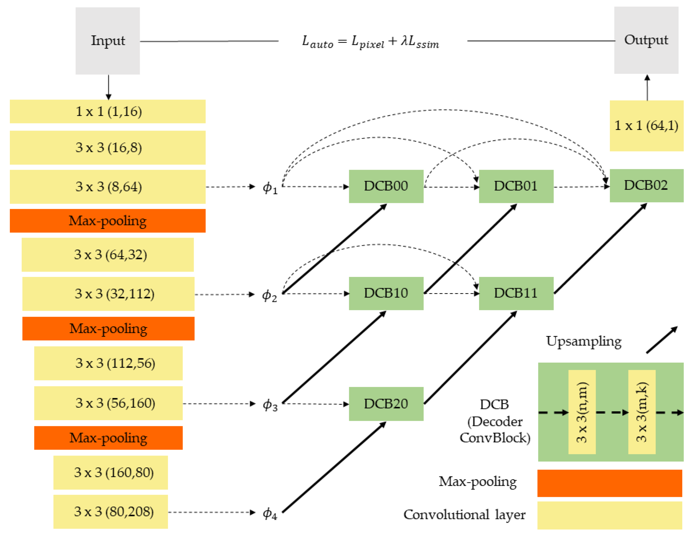
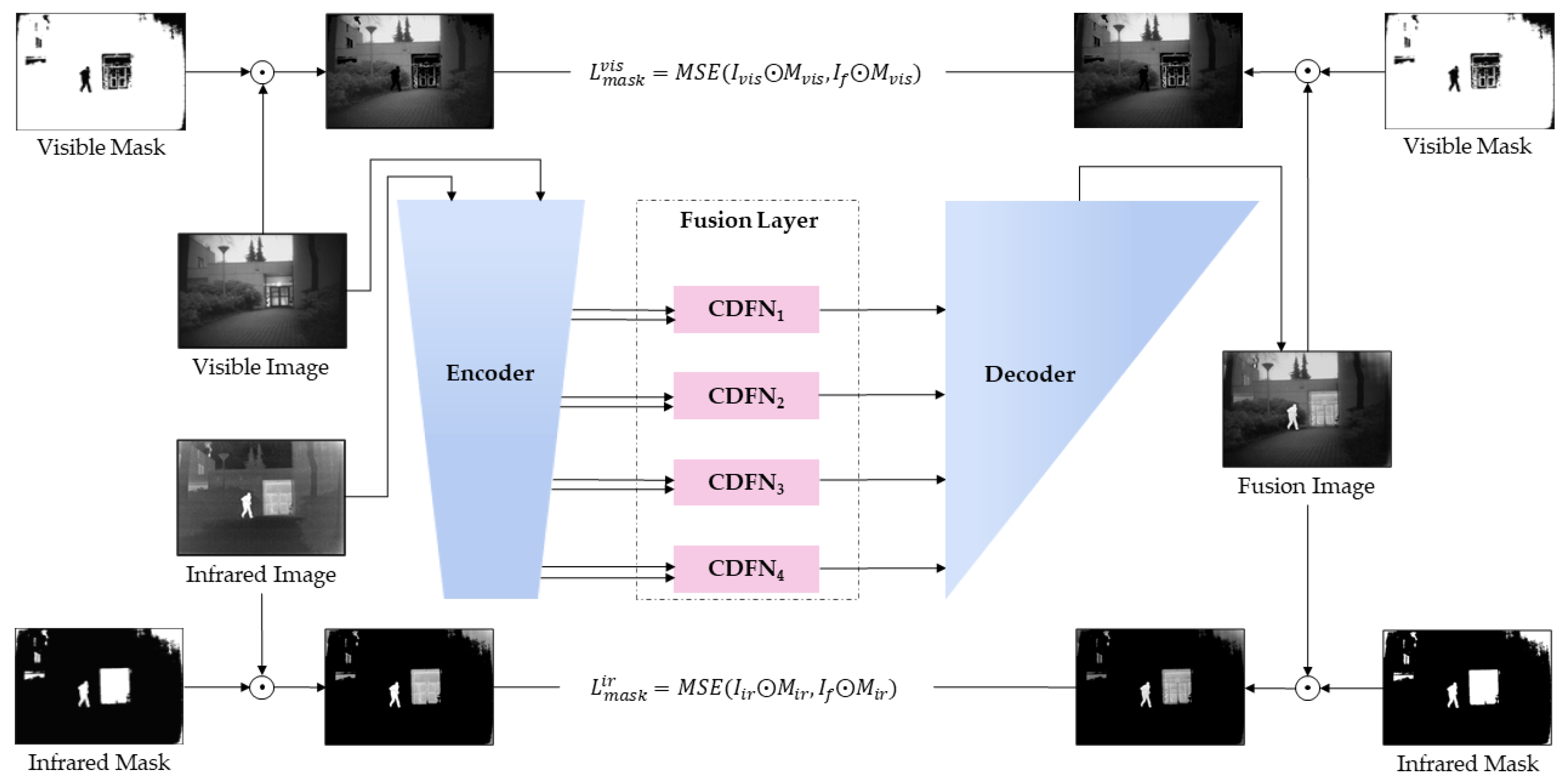
To solve some of the abovementioned problems, this study is based on the Nestfuse [20] network and is further improved to construct an end-to-end multiscale autoencoder network. At the same time, we propose an efficient fusion strategy based on mask and cross-dynamic fusion methods. This strategy enhances the infrared salient features in the image and injects richer texture detail and edge information into the image. The main contributions of this paper are as follows:

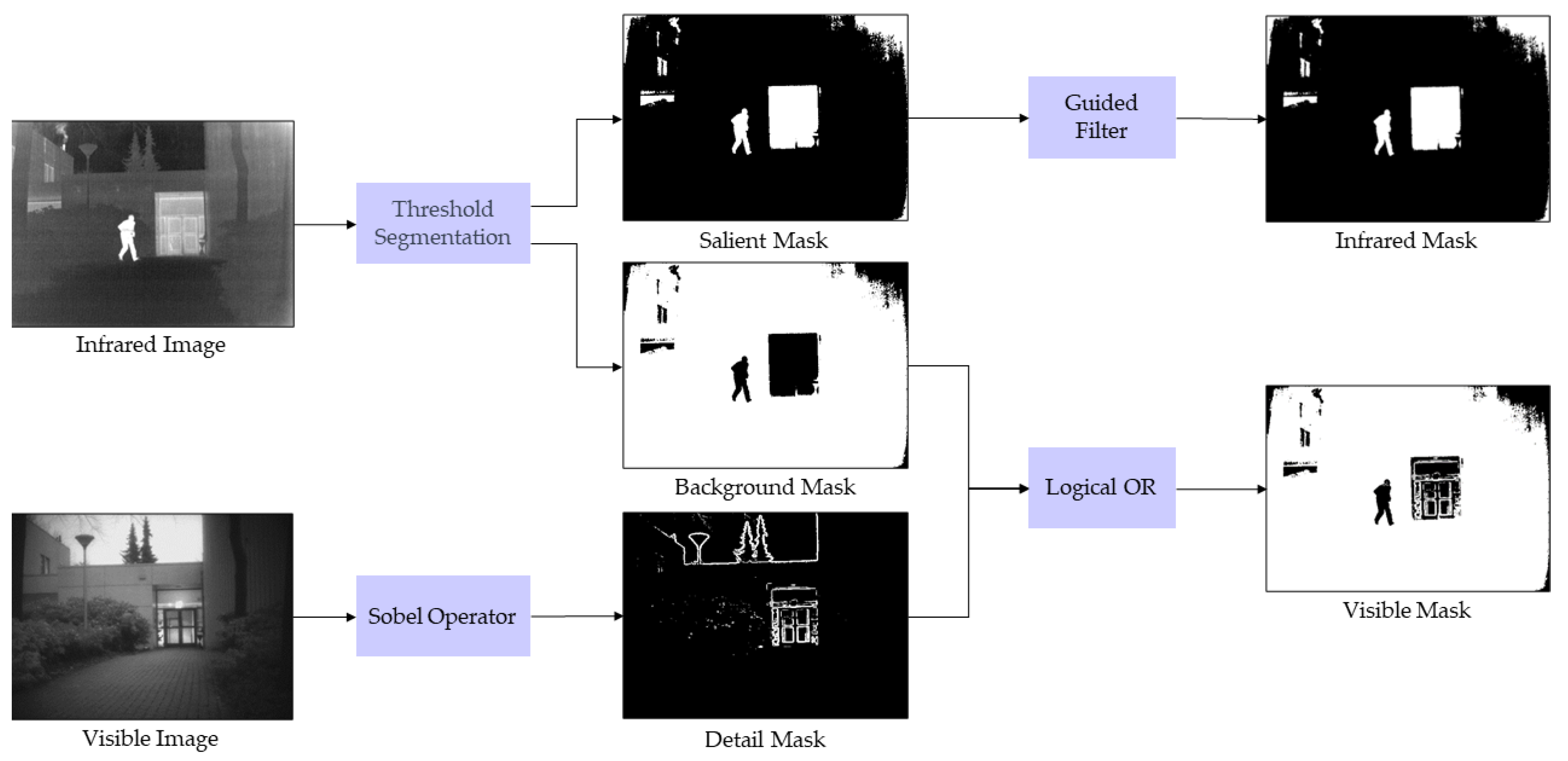
(1) We integrate a novel mask generation strategy in the training stage. The resulting fused image retains the more prominent area features and clearer edge texture information of the source image.

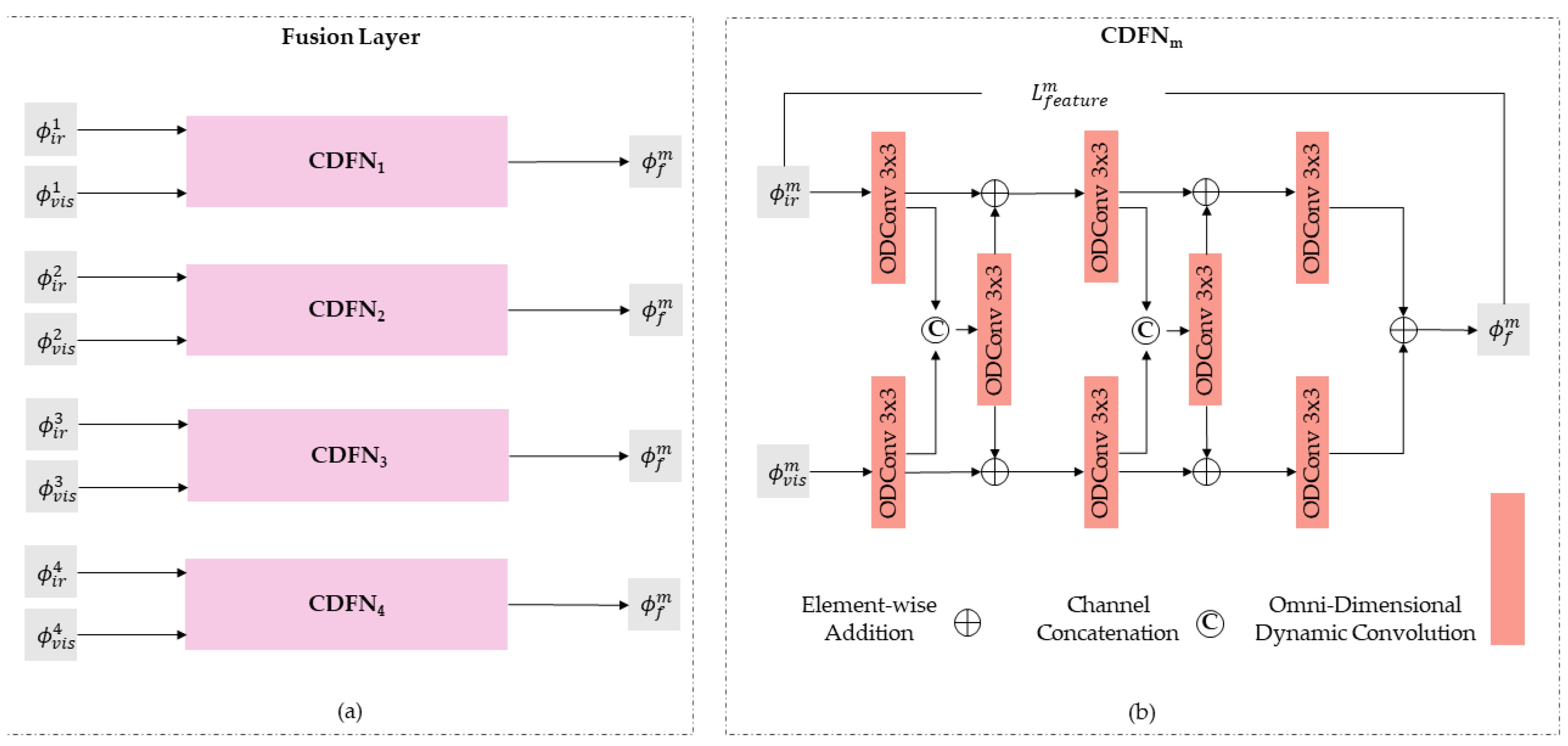
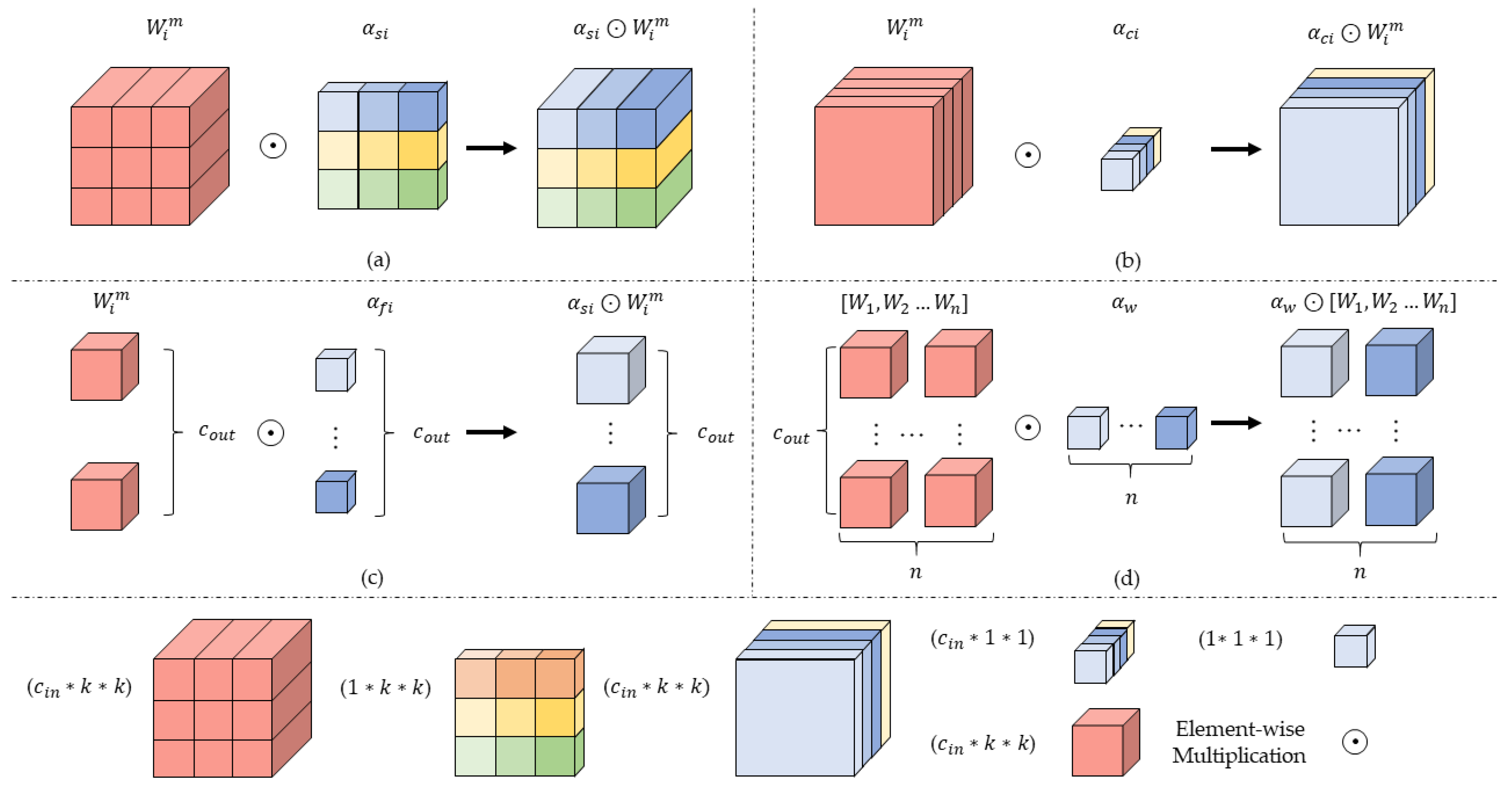
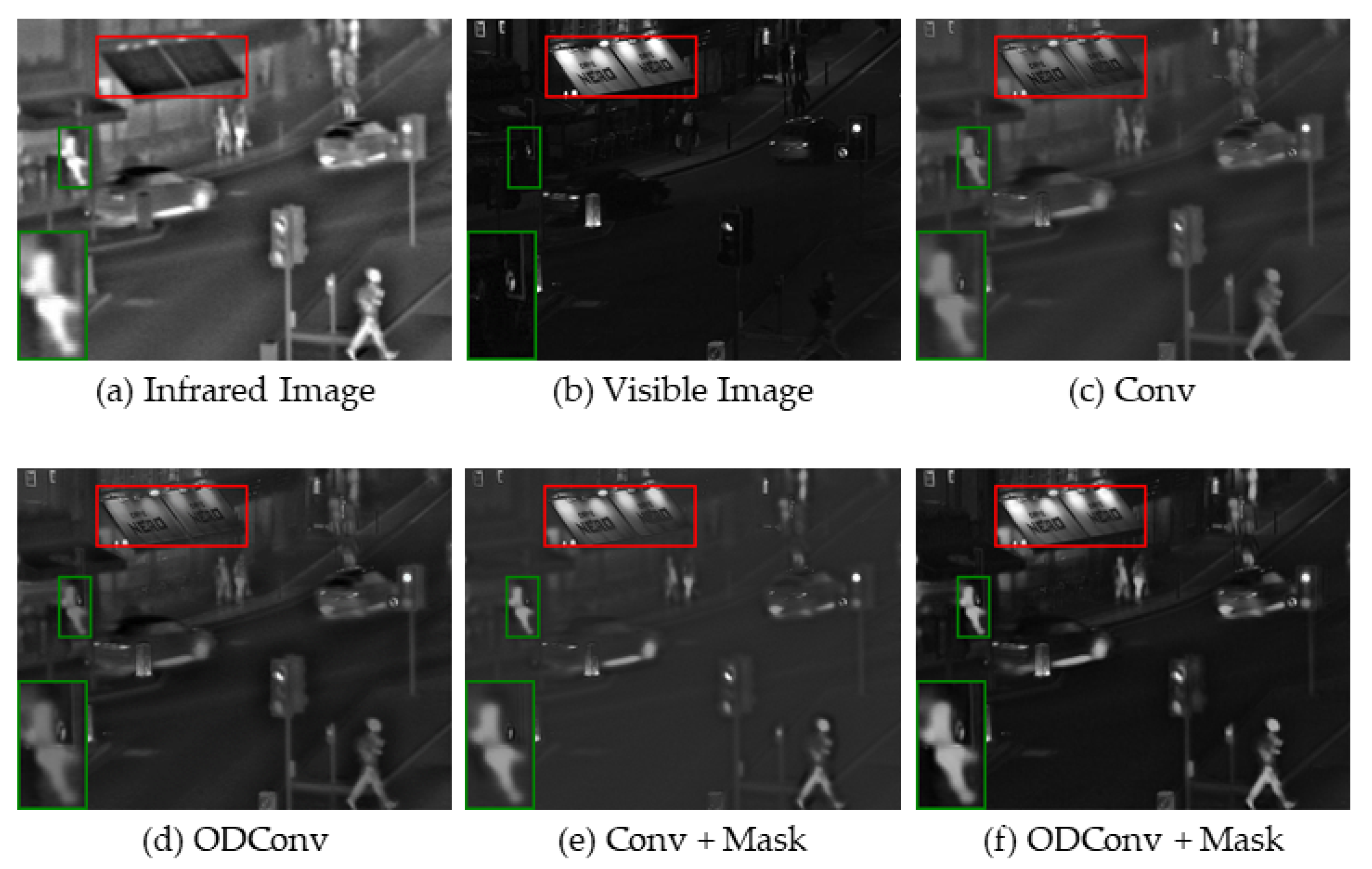
(2) We adopt a cross-dynamic fusion method regarding the fusion layer. In this way, different features in the source images can adaptively fuse in multiple dimensions, further improving the overall fusion effect.

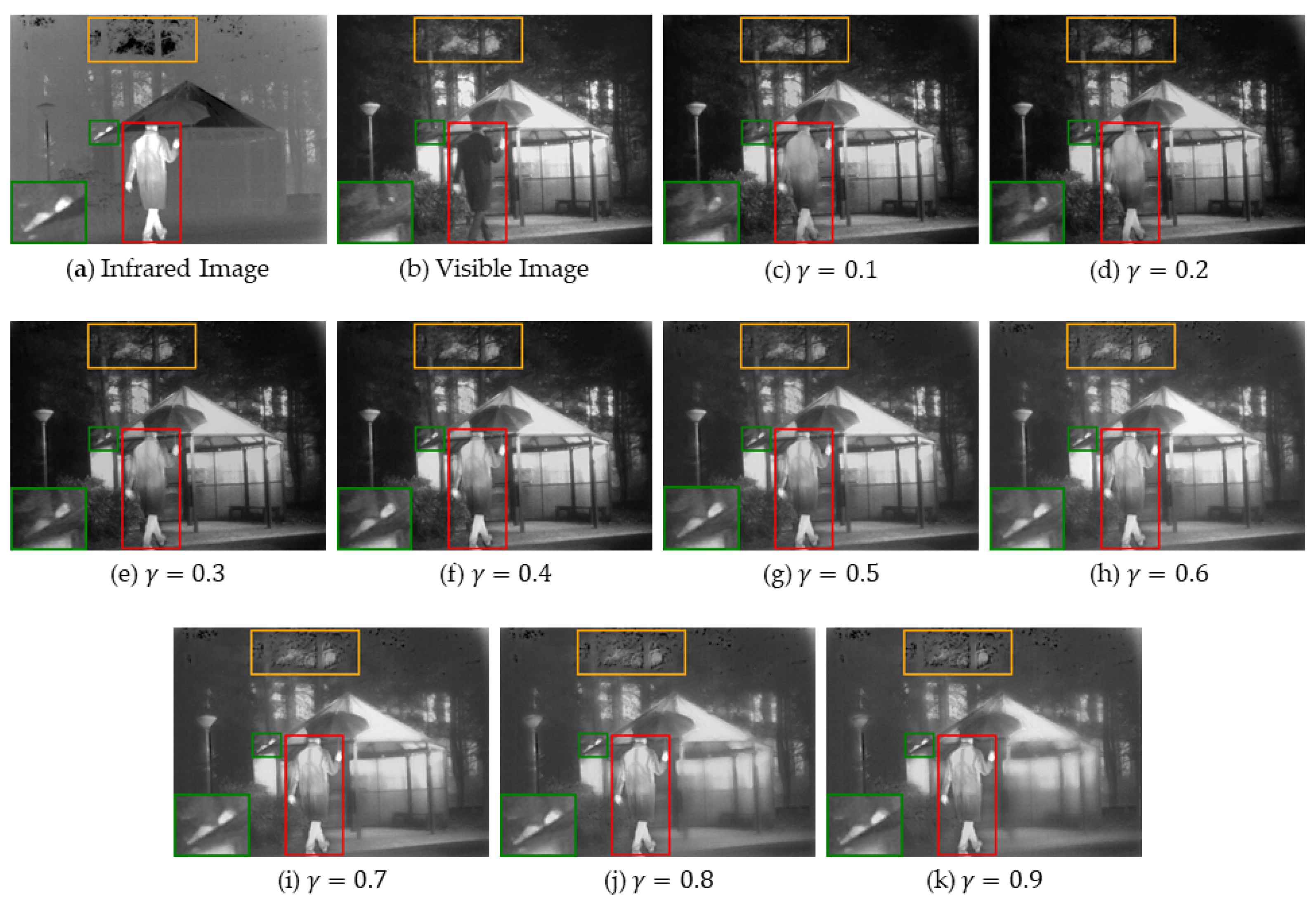
(3) To ensure that the fusion image maintains a mutual balance between retaining rich texture detail and salient features of thermal imaging, we design a blending loss strategy in the fusion stage.

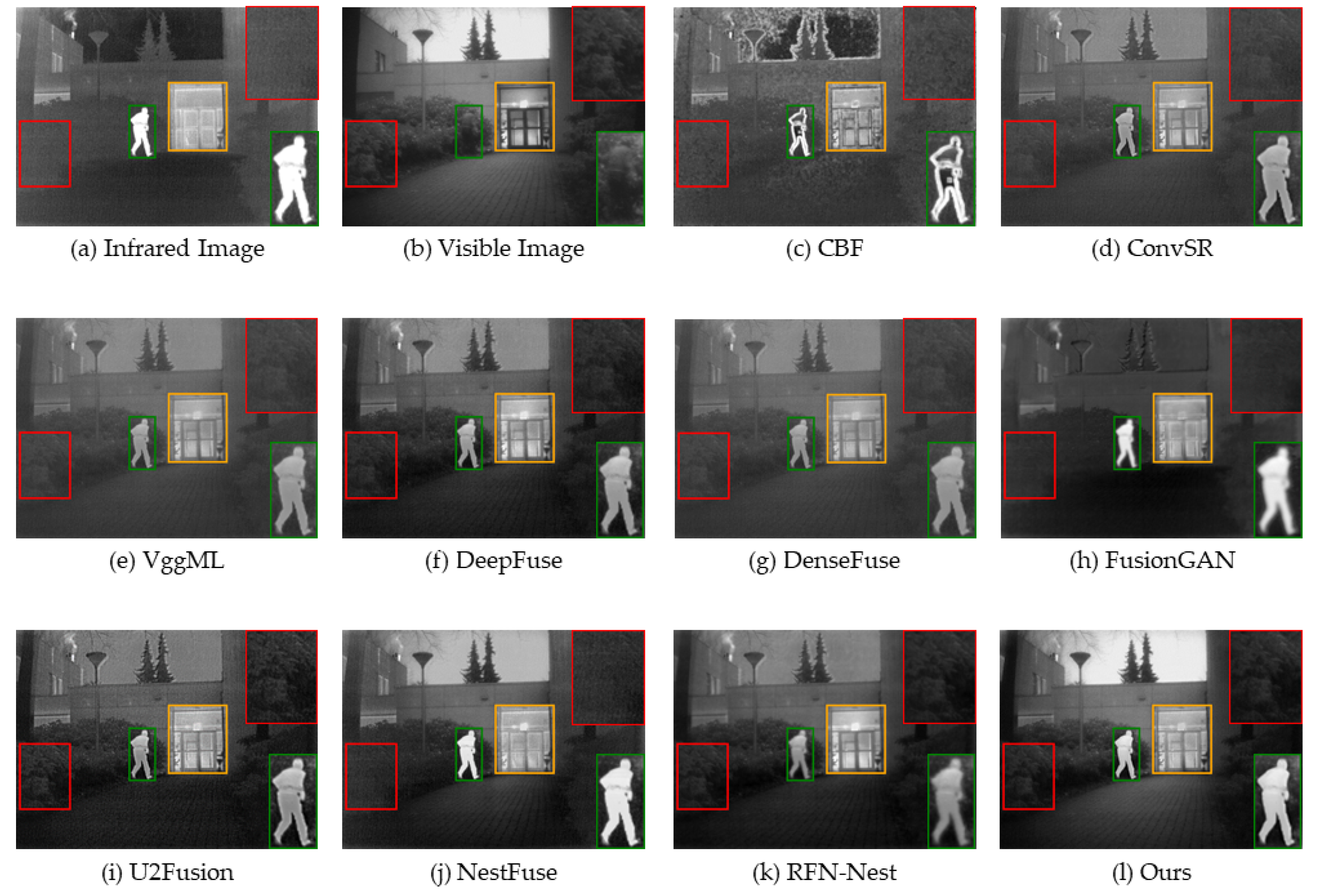
The rest of this article is organized below. Section 2 details the overall framework of MCDFN and training strategies, mask generation strategies, hybrid loss functions, etc. In Section 3, we conduct experiments on the proposed method and evaluate the experimental results to demonstrate the effectiveness and generalization of the proposed method. Finally, Section 4 gives some discussion and conclusions.

2. Materials and Methods

In this paper, we propose an infrared and visible image fusion network structure based on mask and cross-dynamic fusion, including end-to-end autoencoder network structure, two-stage network training, mask generation strategy, cross-dynamic fusion layer designed using omni-dimensional dynamic convolution (ODConv [29]), and the proposed hybrid loss function. In this section, we will cover the above in detail.

2.1. Framework Overview

The shallow feature map mainly captures the low-level features of the image, such as edges, colors, textures, etc. In contrast, the deep feature map can capture the high-level features of the image, including the shape, spatial structure, and semantic information of the object. Therefore, designing a feature extraction network with multiple scales is significant.

Figure 1 shows the proposed network framework, which consists of three parts: the encoder, fusion layer, and decoder. In this network, the encoder’s feature extraction ability and the decoder’s feature reconstruction ability are crucial in generating the final fusion image.

In Figure 1, we adopted a two-stage training strategy [20]. In the first stage, we train the encoder and decoder to build an autoencoder network to realize tefeature extraction and reconstruction of the input image. Through this stage of autoencoder training, we equip the network with effective extraction and reconstruction capabilities for image features. Subsequently, in the second stage, we use the trained autoencoder to train the fusion layer’s cross-dynamic fusion network (CDFN). CDFN integrates infrared features and visible features from different scales by cross-dynamic convolution to compensate for their information differences, thereby promoting a more effective fusion of infrared and visible features.

It is worth noting that we replaced the traditional convolution with ODConv [29] throughout the fusion layer. Compared with traditional convolution, ODConv introduces a multi-dimensional attention mechanism and adopts a parallel strategy, which can learn diverse attention features in four dimensions of the convolutional kernel space.

To better generate the fusion image containing the infrared image’s significant information and the visible image’s clear texture details, we introduce a mask strategy. This strategy uses the mask of the infrared image to enhance the fusion image’s information acquisition ability and highlight the characteristics of infrared thermal imaging. Similarly, using the mask of the visible image enhances the fusion image’s visual perception, ensuring it possesses rich edge and detailed texture characteristics. The fused images produced by networks trained with this masking strategy can contain more important features in infrared and visible images.

2.2. One-Stage Network Training

In the first stage, the encoder network is trained to extract multiscale features, and the decoder network is trained to reconstruct the input image with multiscale features. The autoencoder training framework is shown in Figure 2.

In Figure 2, $Input$ represents the input image and $Output$ represents the output image obtained after being processed and reconstructed through the autoencoder network. The left-side encoder is responsible for extracting deep features, comprising ordinary convolution layers with kernel sizes of 1 × 1 and 31 × 3 and down-sampling operations (max-pooling). When the input image passes through the encoder, it yields deep features at four scales (${\varphi }_{1-4}$). On the right side, the decoder receives the multiscale deep feature maps the encoder provides. These feature maps undergo convolution and up-sampling operations through skip-short connections and are eventually reconstructed into the output image.

In the first stage of autoencoder network training, we use the $L_{auto}$ loss function to train the autoencoder network. This ensures that the output image, obtained after the input image passes through the autoencoder network, can be consistent with the input image. $L_{auto}$ is defined in Equation (1).

$$L_{auto}=L_{pixel}+\lambda L_{ssim}$$

(1)

$L_{pixel}$ and $L_{ssim}$ represent the pixel loss and structural similarity loss between the input and output images, respectively. $\lambda$ is a trade-off value between $L_{pixel}$ and $L_{ssim}$. The formula for calculating the $L_{pixel}$ is shown in Equation (2):

$$L_{pixel}={\left|\right|Output-Input\left|\right|}_F^2$$

(2)

where ${\left|\left|·\right|\right|}_F$ is the Frobenius norm, which measures the error between the output image and the input image, $L_{pixel}$ limits the output image to being as close to the input image as possible at the pixel level.

$L_{ssim}$ is used to limit the structural consistency of the input and output images and improve the robustness of image reconstruction, which is defined as Equation (3):

$$L_{ssim}=1-SSIM\left(Output,Input\right)$$

(3)

where $SSIM(·)$ is a structured similarity measure. This function will calculate the structural similarity between the output and input images; the calculated value ranges between [0, 1]. For $L_{ssim}$, the smaller the value, the closer the structural similarity between the two.

2.3. Fusion Layer Design

We propose an infrared and visible image fusion network structure based on mask and cross-dynamic fusion. This structure includes an end-to-end autoencoder network, a two-stage network training approach, and a mask generation strategy. Furthermore, it features a cross-dynamic fusion layer designed using omni-dimensional dynamic convolution (ODConv [29]) and incorporates our proposed hybrid loss function. In this section, we will delve into these components in detail.

In the fusion layer, we design four scale fusion modules. For each module, a cross-dynamic fusion strategy is employed to integrate multiscale features better. Instead of the standard convolutional layer, we incorporate the ODConv layer in the network. This enhances the feature fusion effect across multiple dimensions, optimizes the important target within the fused image, minimizes interference from irrelevant regions, and reduces redundant information. As a result, our model is versatile, adapting to diverse fusion requirements under various scenarios. The structure of the fusion layer is illustrated in Figure 3a:

In the CDFN module of Figure 3b, ${\varphi }_{ir}^m$ and ${\varphi }_{vis}^m$ represent the mth-scale infrared image feature and the visible image feature extracted by the encoder, where $m\in \{1,2,3,4\}$ corresponds to a multiscale layer 1–4 CDFN network, where all convolutional layers use ODConv. At the same time, in order to retain the effective information of infrared salient feature maps of different scales, we design a multiscale infrared feature loss function ($L_{feature}^m$), where $m\in \{1,2,3,4\}$ represents the feature loss of the layer 1–4 network, ${\left|\left|·\right|\right|}_F^2$ represents the square of the Frobenius norm, and the infrared feature loss function formula is as defined Equation (4):

$$L_{feature}^m={\left|\left|{\varphi }_f^m-{\varphi }_{ir}^m\right|\right|}_F^2$$

(4)

Dynamic convolution was initially proposed in CondConv [30] and DyConv [31]. However, the implementation of the two is different, which also leads to different results in the model’s accuracy, size, and efficiency.

CondConv breaks a fundamental static convolution assumption: all datasets’ samples should use the same convolution kernel. CondConv learns specialized convolution kernels for each input, which opens up a new direction for increasing model capacity while maintaining efficient processing power, increasing the scale and complexity of convolution kernel generation functions. That is, the amount of computation generated by the convolution kernel is more efficient than adding more convolution or more channel counts.

The primary objective of dynamic convolution is to strike a balance between network efficiency and computational demand. Traditional strategies to enhance network performance, such as widening or deepening the network, often lead to increased computational overhead. This is not ideal for networks designed for efficiency. Therefore, DyConv is proposed to solve the problem of expressing capabilities through multi-convolutional kernel fusion models without increasing the depth and width of the network. For dynamic convolutional layers, dynamic convolution uses a dynamic attention mechanism to weighted linear combinations of n convolution kernels to enable the convolution operation of dynamic convolution to be linked to the input data. In CondConv, dynamic convolution is defined as Equation (5):

$$y=\left({\alpha }_1{W}_1+{\alpha }_2{W}_2+\dots +{\alpha }_n{W}_n\right)\ast x$$

(5)

In the above dynamic convolution formula, $x\in R_{in}^{h\ast w\ast c}$ and $y\in R_{out}^{h\ast w\ast c}$ represent the input characteristics and output features (features are represented as R, height is h, width is w, and the number of channels is c); $W_n$ represents a convolution kernel of dynamic convolution, with the same dimensions as the standard convolution kernel parameter. ${\alpha }_n\in R$ is a weighted coefficient learned by gradient descent, calculated using the attention function ${\pi }_{wi}\left(x\right)$ to weight the $W_n$.

Building on CondConv and DyConv, ODConv introduces a multi-dimensional attention mechanism, as shown in Figure 4.

In Figure 4, element-wise multiplication operations are performed in four dimensions, namely the spatial dimension (Figure 4a), the input channel dimension (Figure 4b), the output channel dimension (Figure 4c), and the convolution dimension of the convolution kernel space (Figure 4d). All four attentions are calculated using the long attention mechanism. Dynamic convolution in ODConv is defined as Equation (6):

$$y=\sum _{k=1}^n({\alpha }_{s}k\odot {\alpha }_{c}k\odot {\alpha }_{f}k\odot {\alpha }_{w}k\odot W_k)\ast x$$

(6)

where the symbols x and the symbol y are the same as Equation 5, ${\alpha }_{wi}\in R$ represents the attention weight coefficient of the convolution kernel $W_i$; ${\alpha }_{si}\in R^{k\ast k}$, ${\alpha }_{ci}\in R^{c_{in}}$, ${\alpha }_{fi}\in R^{c_{out}}$ represent the attention calculation weight coefficients of the spatial dimension, input channel dimension, and output channel dimension, respectively; and ⊙ represents element-wise multiplication operations in different dimensions. ${\alpha }_{si}$, ${\alpha }_{ci}$, ${\alpha }_{fi}$, ${\alpha }_{wi}$ are all calculated here by the multi-head attention module ${\pi }_{wi}\left(x\right)$. ODConv’s attention to the four dimensions is complementary, providing performance guarantees for obtaining rich contextual information.

2.4. Mask Generation Strategy

Using masks to limit the fusion process can help improve fusion quality and visual perception fidelity. Infrared masks can help models identify salient objects or features in infrared images, focusing attention on the most important areas of infrared images. By using infrared masks, the model can suppress noise and irrelevant information in infrared images, thereby improving the degree of concentration on infrared information. Visible masks are used to highlight the shape and texture details of objects in visible images. They improve the visual quality of the fused image, bringing it closer to the appearance of the visible image. By emphasizing visible detail, the contrast of the fused image can be increased, resulting in a more recognizable and visually natural image.

The generation process of the infrared mask and the visible mask used in our model is illustrated in Figure 5.

Considering that different target areas in infrared and visible images have different pixel brightness values, a method combining threshold segmentation, a guided filter, and a Sobel operator generates masks corresponding to infrared and visible images. First, we obtain threshold segmentation masks for infrared images and visible images, which are generated as follows:

$$M_{i{r}_{ij}}=\left\{\begin{array}{c}1,I_{i{r}_{ij}}-{\overline{I}}_{ir}>threshold\hfill \\ 0,otherwise\hfill \end{array}\right.$$

(7)

where $M_{{ir}_{ij}}$ and $I_{i{r}_{ij}}$ are the pixel values of the infrared significant mask $M_{ir}$ and the infrared image $I_{ir}$, respectively, in row i and column j; ${\overline{I}}_{ir}$ is the average of all elements in the $I_{ir}$, $threshold$ is the predefined threshold, and in the same way, we can obtain the visible background mask $M_{vis}=1-M_{ir}$. Based on the empirical design in the related article [32,33], the $threshold$ is set to 50 in this article.

Secondly, to emphasize the essential details in the infrared image and the intricate texture in the visible image, We employed a guide filter [34]. This filter method was to soften the starkness of the edges, even out the mask image, and accentuate the target within the picture. In addition, we use the Sobel operator to process the visible original image, and by highlighting the edge area, we can obtain a visible edge texture mask with high-frequency texture information characteristics. The Sobel operator is shown in Equation (8):

$$\begin{array}{cc}\hfill & \hfill G_{vis}^x=\left[\begin{array}{ccc}-1& 0& 1\\ -2& 0& 2\\ -1& 0& 1\end{array}\right]\ast I_{vis}\hfill \\ \hfill & \hfill G_{vis}^y=\left[\begin{array}{ccc}-1& -2& -1\\ 0& 0& 0\\ 1& 2& 1\end{array}\right]\ast I_{vis}\hfill \\ \hfill & \hfill M_{vis}=\sqrt{{G_{vis}^x}^2+{G_{vis}^y}^2}\hfill \end{array}$$

(8)

Among them, $G_{vis}^x$ is used to detect vertical edges, $G_{vis}^y$ is used to detect horizontal edges, and $M_{vis}$ is the final generated visible detail mask.

Finally, logical OR operations are applied to the visible background mask and visible detail mask to obtain the final visible mask used for training. All masks used in this dataset are generated using this mask generation strategy.

2.5. Two-Stage Network Training

In the second stage, the encoder and decoder are fixed after training in the first stage, using the infrared feature loss function to train the fusion network (CDFN). Meanwhile, we added an infrared mask and a visible mask to enhance the fusion image information to retain important information in the mask area in the infrared and visible image. Figure 1 shows the second stage of the training process.

In Figure 1, we use a trained encoder network to extract depth features from the source image. Feature maps (${\varphi }_{ir}^m$ and ${\varphi }_{vi}^m$) at different scales are input into multiple CDFNs designed by us in pairs, and fusion is carried out at different scales. Finally, through the trained decoder network, the fusion feature image (${\varphi }_f^m$) obtained at multiple scales is reconstructed into the final fusion image.

To train MCDFN, we propose a $L_{MCDFN}$ of mixed loss functions, which is defined as Equation (9):

$$L_{MCDFN}={L_{mask}+\alpha L}_{feature}+\beta L_{ssim}$$

(9)

$L_{mask}$, $L_{feature}$, and $L_{ssim}$ represent the mask content loss function, infrared feature loss function, and structural similarity loss function, respectively, and $\alpha$ and $\beta$ are the weights set to balance the influence of the loss function on the image. $L_{mask}$ contains infrared mask loss ($L_{mask}^{ir}$) and visible mask loss ($L_{mask}^{vis}$), defined as Equation (10):

$$L_{mask}^{ir}=MSE\left(I_{ir}\odot M,I_f\odot M\right)$$

(10)

where $MSE$ represents the mean squared error function, $I_{ir}\odot M$ is used to represent significant features in infrared images, $I_f\odot M$ is used to represent significant features in fused images, and similarly, texture details and structural information in visible images can be expressed as Equation (11),

$$L_{mask}^{vis}=MSE(I_{vis}\odot (1-M),If\odot (1-M))$$

(11)

Combining $L_{mask}^{ir}$ and $L_{mask}^{vis}$ yields the total loss function $L_{mask}$, expressed as Equation (12).

$$L_{mask}=L_{mask}^{ir}+L_{mask}^{vis}$$

(12)

$L_{feature}$ represents the multiscale infrared feature loss function, which is used to constrain the deeper features to retain a more significant structure because infrared images have different significant target features at different scales. $L_{feature}$ is defined as Equation (13):

$$L_{feature}=\sum _{m=1}^4{w}_m{L}_{feature}^m$$

(13)

In Equation (13), we use $w_m$ as the weights for different scale loss functions due to the variations in the fusion layers at different scales. According to the loss ratio, we set $w_m=[1,10,100,1000]$, and the formula for $L_{feature}^m$ can be found in Equation (4).

To reflect the structural information between the generated image and the source image, we also introduce structural similarity loss to preserve further the structural similarity between the generated and the source images. $L_{ssim}$ is defined as follows:

$$L_{ssim}=\gamma (1-SSIM(I_{ir},I_f))+(1-\gamma )(1-SSIM(I_{vis},I_f))$$

(14)

where $\gamma$ is used to balance the similarity between a fused image and a different source image.

3. Experiments and Results Analysis

This section briefly describes the experimental setup, including the training and test experiment setup and the parameter settings and evaluation metrics used during the testing stage. Secondly, we conduct ablation experiments on the module and loss function weight design in the MCDFN model to verify the necessity of each module and weight design. Finally, we qualitatively compare the MCDFN model with other existing fusion models on the public test sets TNO [35] and RoadScene [36]. In addition, we use seven different types of public evaluation metrics to objectively evaluate the fusion performance of each model to ensure that the validity of the MCDFN model is demonstrated in qualitative and quantitative comparisons.

3.1. Experimental Setup and Implementation

3.1.1. Network Training Settings

Our model training consists of two stages: In the first stage, we train an encoder-decoder network to extract multiscale depth features of images and reconstruct them. 80,000 images of the MS-COCO dataset were used for training, and these images were converted into a 256 × 256 grayscale map. In Equation (1), to make the $L_{pixel}$ and $L_{ssim}$ have similar orders of magnitude, we set the value of the parameter $\lambda$ to $1\times {10}^2$. The number of epochs, learning rate, and batch size are set to 2, $1\times {10}^{-4}$, and 4, respectively.

In the second stage, we select some images from the KASIT [37] dataset, process these images, adjust the resolution to 224 × 224, and obtain 27,000 pairs of infrared and visible grayscale maps, and at the same time, through the infrared mask generation strategy in Equation (7), the 27,000 filtered infrared grayscale images are processed to obtain the same number of infrared masks and visible masks. Figure 1 shows the two-stage training process, in which the autoencoder after the one-stage training is fixed, and the mask and fusion layer are introduced to further train the network. In the second stage of training, the number of epochs, learning rate, and batch size are set to 10, $1\times {10}^{-3}$, and 8, respectively.

Our experiments were conducted on the Linux operating system using NVIDIA RTX 3090, programming environments for Python 3.8 and Pytorch 1.7.1, and CUDA version 11.0.

3.1.2. Test Experiment Setup

Our model was tested using two public test datasets: the TNO dataset, consisting of 21 pairs of infrared and visible images, and the RoadScene dataset, consisting of 43 pairs of infrared and visible images. The TNO dataset is one of the most commonly used datasets for research in infrared-visible image fusion. It includes various multi-spectral images taken under conditions such as indoor and outdoor environments, low-light scenarios, adverse weather, and natural subjects like humans, machinery, vehicles, and buildings. The RoadScene dataset comprises registered visible and infrared images sourced from genuine driving recordings. These paired images capture quintessential road environments teeming with pedestrians and vehicles.

3.1.3. Evaluation Metrics

Even without ground-truth for each image pair, various quantitative metrics remain available for image fusion assessment. In this article, we use seven evaluation metrics, which are grouped into the following five categories:

(1) Evaluation metrics based on information theory: entropy (EN [38]), mutual information (MI [39]), fusion mutual information weighted (FMI${}_w$ [40]);

(2) Evaluation metrics based on image features: standard deviation (SD [38]);

(3) Evaluation metrics based on structural similarity: structural similarity index measure (SSIM [41]);

(4) Evaluation metrics based on human visual perception: visual information fidelity (VIF [42]);

(5) Evaluation metrics based on source and generated images: gradient-based fusion performance (Q${}^{AB/F}$ [43]).

Higher values for EN, MI, and SD indicate that the image has richer texture and detail, contains more information from the other image, and has greater contrast within the image. An increase in FMI${}_w$ suggests a stronger similarity of the two images at the feature level. A rise in SSIM indicates that the two images are visually more similar. A higher VIF value indicates better visual fidelity of the image, aligning more with human visual habits. As for Q${}^{AB/F}$, it measures the degree to which salient information between the images is expressed. A higher Q${}^{AB/F}$ value indicates better quality of the salient information in the fused image.

In summary, the higher the values of the above seven indicators, the better the performance of the fused image in terms of information volume, visual perception, and overall fusion effect. However, we must recognize that these assessment indicators are often subject to their constraints and limitations and that there may be mutual constraints between them. Therefore, based on specific application needs, we should weigh the advantages and limitations of these metrics to optimize and train the model to ensure that the model can achieve the best results in the actual application.

3.2. Ablation Experiments

In this section, we delve into the impact of the $\alpha$ and $\beta$ parameters within $L_{MODFN}$ and the significance of the $\gamma$ parameter in $L_{ssim}$ on fusion efficacy. We will also shed light on the robustness and relevance of the infrared masking technique and the utility of the ODConv module. For clarity, all experimental references in this discussion are based on evaluations conducted using 21 pairs from the TNO dataset.

3.2.1. The Effect of the Loss Function Weights

Regarding the three weight parameters ($\alpha$, $\beta$, $\gamma$) within the loss function presented in this paper, during comparative experiments, one parameter is analyzed while keeping the other two fixed. To begin with, based on the loss ratio in the training process, we set both $\alpha$ and $\beta$ to a fixed value of 0.1. Then, the $\gamma$ weight values are compared, with $\gamma$ ranging from 0.1 to 0.9. Figure 6 shows the fusion results for these different $\gamma$ weights. Feature details in smaller color boxes are enlarged to larger same-color boxes in the same image. Annotations in subsequent figures follow the same pattern.

Observing Figure 6, it is evident that as the value of $\gamma$ increases, the texture details of the “tree” (within the orange box) gradually diminish. Concurrently, the infrared information of the “person” (within the red box) becomes more pronounced. Furthermore, the distinct objects within the “green box” become progressively clearer, while the background visible information increasingly blurs. It is readily apparent that when $\gamma$ falls within the range of {0.1, 0.2}, the amalgamated image places undue emphasis on preserving the structural and textural nuances of the visible snapshot. This tendency inadvertently sacrifices a considerable volume of infrared image intricacies. On the flip side, for $\gamma$ values in the vicinity of {0.8, 0.9}, the fusion becomes skewed towards safeguarding infrared data, which manifests as pronounced noise around the “tree” and a palpable erosion of texture throughout the picture. Fusion images obtained with $\gamma$ values in the range of {0.3, 0.4, 0.5, 0.6, 0.7} can decently retain the complementary information between the source images. Thus, our consideration narrows down to selecting from these five weight values.

We objectively evaluated the influence of these $\gamma$ values on the fusion images, and the fusion assessment indicators corresponding to different $\gamma$ values are presented in

Table 1. Evaluation results of the five $\gamma$ values on the 21 pairs of the TNO dataset.

$\mathit{\gamma }$	EN	SD	MI	FMI${}_{\mathit{w}}$	SSIM	VIF	Q${}^{\mathbf{AB}/\mathit{F}}$
0.3	7.022	100.319	14.044	0.425	0.664	0.940	0.484
0.4	7.055	102.314	14.110	0.422	0.679	0.927	0.471
0.5	7.043	101.701	14.087	0.412	0.687	0.870	0.452
0.6	7.012	101.434	14.065	0.393	0.695	0.794	0.416
0.7	7.026	98.127	14.052	0.391	0.697	0.716	0.367

. The bold font, italic font, and underlined font represent each column’s best value, second-best value, and third-best value. Annotations in subsequent tables follow the same pattern.

Table 1 shows that when $\gamma$ is set to 0.4, it achieves three best and three second-best values. Consequently, we fix $\gamma$ at 0.4 for subsequent comparative experiments involving $\alpha$ and $\beta$. Firstly, with $\alpha$ fixed at 0.1 and $\gamma$ at 0.4, we set $\beta$ to values within {0.01, 0.1, 1}. Subsequently, with $\beta$ fixed at 0.1 and $\gamma$ at 0.4, we set $\alpha$ to values in {0.01, 0.1, 1}. Quantitative comparison results are presented in

Table 2. Evaluation results of different $\alpha$ and $\beta$ values on the 21 pairs of the TNO dataset.

$\mathit{\alpha }$	$\mathit{\beta }$	EN	SD	MI	FMI${}_{\mathit{w}}$	SSIM	VIF	Q${}^{\mathbf{AB}/\mathit{F}}$
0.1	1	6.874	90.236	13.749	0.425	0.697	0.826	0.429
	0.1	7.055	102.314	14.110	0.422	0.679	0.927	0.471
	0.01	7.039	100.761	14.079	0.382	0.655	0.896	0.457
1	0.1	7.015	100.747	14.051	0.411	0.659	0.962	0.470
0.01	0.1	6.992	99.106	13.985	0.429	0.649	0.925	0.469

.

In Table 2, the weights of $\alpha$ = 0.1, $\beta$ = 0.1, and $\gamma$ = 0.4 yielded four best values, two second-best values, and one third-best value. In summary, after qualitative and quantitative evaluation, we believe that the network trained with this combination of weight coefficients can have better fusion performance. Subsequent experiments will be conducted under this combination of weight coefficients.

3.2.2. Effect of Masks and ODConv Modules

To verify the impact of the mask and the ODConv module on our proposed model, we conducted ablation studies on both components during the two-stage training process. Without the mask, the content in Equation (12) related to $L_{mask}$ is replaced with $MSE(I_{ir},I_f)+MSE(I_{vis},I_f)$ to balance the disparity between the source and fused images. We compared the fusion networks in different scenarios: without any added modules (only ordinary Conv), with only the mask module added, with only the ODConv module added, and with both the mask and ODConv modules integrated. Comparison illustrations can be found in Figure 7.

In Figure 7, the fusion image (d) using ODConv has clearer edge information and texture detail in the background content compared to the fusion image (c) using Conv. The fusion image generated by Conv and mask in (e) can retain more prominent “person” (within the green box) features and improve the visibility of “text” (within the red box). Finally, the fusion image generated by combining ODConv and mask in (f) has rich background edge information and texture details. It retains crucial infrared image features, thereby significantly improving visual perception.

In

Table 3. Evaluation results of different modules on the 21 pairs of the TNO dataset.

	EN	SD	MI	FMIw	SSIM	VIF	Q${}^{\mathbf{AB}/\mathit{F}}$
Conv	6.707	66.450	13.414	0.419	0.709	0.746	0.427
ODConv	6.741	67.529	13.482	0.423	0.713	0.761	0.426
Conv + Mask	6.827	92.065	13.655	0.424	0.685	0.886	0.449
ODConv + Mask	7.055	102.314	14.110	0.422	0.679	0.927	0.471

, the comparison of quantitative evaluation indicators across four different module combinations is presented. When contrasted with the traditional Conv fusion network, the fusion image incorporating the mask module exhibits a marked improvement in index performance. While adding only the ODConv module does not lead to a significant rise in the fusion index compared to the traditional Conv, introducing both the mask module and ODConv module surpasses the performance of only using the mask module. There is a notable enhancement in EN, SD, MI, VIF, Q${}^{AB/F}$ indicators. This can be attributed to the mask module allowing the ODConv to capitalize on its multi-dimensional attention characteristics more efficiently. Consequently, this leads to an adaptive enhancement across spatial and channel dimensions, emphasizing specific features like edges, textures, or salient objects, thereby improving image visibility and prominence of features.

3.3. Qualitative and Quantitative Evaluation on TNO Dataset

We compared our proposed MCDFN model with nine representative methods on the TNO dataset in both qualitative and quantitative aspects. These methods include the fusion method based on Cross-Bilateral Filtering (CBF [44]), the fusion method based on Convolutional Sparse Representation (ConvSR [45]); the Multi-Layer Deep Feature Fusion method (VggML [46]); DeepFuse [47]; the fusion method based on Dense Block (DenseFuse [19]); the fusion method based on Generative Adversarial Networks (FusionGAN [21]); U2Fusion [26]; the fusion method based on Nested Connection NestFuse [20], and RFN-Nest [48].

Figure 8 and Figure 9 are the experimental results of various methods on test images (’Kaptein_1123’ and ’Dune’) of different TNO datasets, respectively. In order to better evaluate the qualitatively between different fusion methods, we use red boxes, green boxes, and orange boxes to label the more obvious feature areas.

From Figure 8, it can be observed that although CBF can show the infrared features of the “person” in the green box, it only highlights the edge area of the “person”, and the texture details of the “grass” in the red box are basically invisible. ConvSR, VggML, DeepFuse, DenseFuse, U2Fusion, and RFN-Nest can highlight the overall salient features of a “person”, but compared with infrared images, their features are still relatively gray, and the “grass” detail features of ConvSR, VggML, and DenseFuse are seriously lost. In addition to CBF, FusionGAN, and NestFuse, other methods and our method can better retain the edge information of the “door frame” in the orange box. The images obtained by FusionGAN, NestFuse, and our method can all have significant information close to the “person” in the infrared image. However, the information retention of FusionGAN and NestFuse in the “grass” detail is still poor, and the fusion image generated by FusionGAN is closer to the infrared image. Our method retains the infrared salient features of the “person” and the texture details of the “grass”, and the edge information in the “door frame” is preserved, which has an excellent visual effect.

In another test, Figure 9, it can be observed that ConvSR, VggML, DenseFuse, and RFN-Nest are unable to clearly showcase the infrared details of the “person” in the red box, with only the upper part of the infrared feature being relatively clear. FusionGAN essentially loses the information of the “fence” in the green box and the overall visible background information. While U2Fusion retains the image features of both the “person” and the “fence”, its background noise is excessive. CBF, DeepFuse, NestFuse, and our method present a smoother image with less noise, preserving many image features from the “person” and “fence”. When retaining the information of the “person” and “fence”, our method is closer to the original infrared and visible images.

Based on the aforementioned comparative analysis, we subjectively believe that, compared to the other nine fusion methods, our method can offer clearer infrared contrast, maintain a higher fidelity in texture visual information, and emphasize the edge features of background information. To further validate the effectiveness of our model, apart from conducting qualitative evaluations of various methods, we also carried out quantitative comparisons on the TNO dataset. The quantitative results of the different methods can be found in

Table 4. Quantitative results of different methods on the 21 pairs of the TNO dataset.

	EN	SD	MI	FMI${}_{\mathit{w}}$	SSIM	VIF	Q${}^{\mathbf{AB}/\mathit{F}}$
CBF	6.857	76.824	13.714	0.323	0.599	0.718	0.453
ConvSR	6.258	50.743	12.517	0.383	0.753	0.633	0.534
VggML	6.182	48.157	12.365	0.416	0.778	0.295	0.451
DeepFuse	6.699	68.793	13.398	0.424	0.728	0.779	0.437
DenseFuse	6.173	47.819	12.347	0.417	0.779	0.608	0.343
FusionGAN	6.362	54.357	12.725	0.370	0.653	0.453	0.218
U2Fusion	6.757	64.911	13.514	0.362	0.694	0.751	0.424
NestFuse	6.894	80.372	13.789	0.432	0.714	0.752	0.483
RFN-Nest	6.841	71.899	13.682	0.302	0.699	0.657	0.359
Ours	7.055	102.314	14.110	0.422	0.679	0.927	0.471

.

As seen from Table 4, our method achieves four best values and two third-best values compared to other methods. The EN, SD, and MI are much greater than the results of other methods, indicating that the fusion image produced by the proposed fusion method contains more information and detail, reflecting its greater advantages in diversity, texture richness, and information retention. VIF is much higher than other methods, indicating that our method has a more significant effect on fusing infrared and visible image features, and the overall vision is closer to the original image.

3.4. Qualitative and Quantitative Evaluation on RoadScene Dataset

To verify the generalizability of our model, we compared our method with the nine methods from Section 3.3 using the same evaluation metrics on the RoadScene dataset. Figure 10 and Figure 11 are the fusion effects of two pairs of infrared and visible images selected on the RoadScene dataset in different methods.

A qualitative evaluation of Figure 10 reveals significant differences between the different methods in the retention of infrared signature information for “people” (within the red box). Specifically, FusionGAN and RFN-Nest are slightly inadequate, resulting in the ambiguity of the infrared characteristics of “people”. At the same time, looking at the texture detail of the “text” (within the green box), we notice that the CBF method loses some of the details. Although ConvSR, VggML, DeepFuse, and DenseFuse retain the texture of “text” to some extent, their low brightness makes the visual effect less than ideal. Impressively, U2Fusion, NestFuse, and the methods proposed in this study excel at preserving “text” details, successfully capturing rich information, and human visual sense. Finally, besides this paper and NestFuse, other fusion images generate artifacts or noise in the background. This further highlights our proposed method’s efficient fusion performance.

In Figure 11, we observe that methods other than FusionGAN and RFN-Nest retain the infrared signature of “human” in the red box well. However, CBF’s background information is still littered with many noise points. In addition, CBF and FusionGAN tried to preserve the details of the “billboard” inside the green box, but there were some artifact effects. In NestFuse, the “billboard” information is almost completely lost. In contrast, our method and VggML, DeepFuse, DenseFuse, and U2Fusion all demonstrate superior performance in maintaining the infrared signature of the “human” and the detail of the “billboard”.

Table 5. Quantitative results of different methods on the 43 pairs of the RoadScene dataset.

	EN	SD	MI	FMI${}_{\mathit{w}}$	SSIM	VIF	Q${}^{\mathbf{AB}/\mathit{F}}$
CBF	7.397	74.974	14.415	0.370	0.624	0.649	0.514
ConvSR	7.035	57.831	14.070	0.388	0.722	0.735	0.589
VggML	6.988	55.660	13.976	0.426	0.717	0.724	0.487
DeepFuse	7.156	63.983	14.312	0.433	0.705	0.753	0.495
DenseFuse	7.224	64.155	14.448	0.390	0.695	0.751	0.484
FusionGAN	7.040	58.950	14.080	0.277	0.598	0.590	0.251
U2Fusion	7.162	60.603	14.324	0.391	0.695	0.713	0.513
NestFuse	7.370	76.136	14.541	0.390	0.668	0.867	0.495
RFN-Nest	7.317	69.510	14.604	0.271	0.657	0.743	0.304
Ours	7.405	78.301	14.610	0.399	0.655	0.786	0.427

presents the evaluation results of different methods on 43 pairs of RoadScene datasets. Remarkably, this paper obtained three best values, one second-best value, and one third-best value in quantitative evaluation. NestFuse and our method perform well on all four indicators: EN, SD, MI, and VIF. This shows that the two methods can better combine thermal radiation information in infrared images with rich textures in visible images. Compared to other methods, they achieve a higher level of background information balance, free of noise and artifacts and more in line with the perception of the human eye. However, although the CBF method achieved two second-best and two third-best values, its excessive reliance on hand-designed fusion methods led to a loss of texture detail in visible images.

The proposed method performs well in all evaluation dimensions after in-depth comparison and evaluation with nine different fusion methods on two datasets. This method can not only accurately capture and retain rich image information and realize the efficient balance and fusion of feature information, but also can preserve the significant infrared characteristics and visible texture details. In addition, it shows good generalization ability, which is undoubtedly more competitive than many other representative fusion technologies.

4. Discussion and Conclusions

This paper proposes a two-stage network structure of binding mask and cross-dynamic fusion, called MCDFN, for infrared and visible image fusion. We design ensemble strategies using convolutional neural networks compared to traditional fusion methods. The mask strategy maximizes the retention of useful information on significant and marginal areas in infrared and visible images. Additionally, we can maximize the fusion of useful information by introducing omni-dimensional dynamic convolution and focusing on the structural features of infrared and visible images across multiple dimensions. We also employ the multiscale infrared feature loss function and the structured similarity loss function to improve the significance and consistency between the generated and original images. Qualitative and quantitative evaluation results with the other nine methods on the TNO and RoadScene datasets show that our fusion method has better feature and detail retention capabilities.

We must acknowledge that, like many others, our model only achieves relatively best results on some datasets or tasks. Furthermore, given the inherent limitations in the field of image fusion, the source images used by our model must be pre-registered. MCDFN employs a multiscale approach that excels at extracting depth features at various scales of images. This enriches the contextual information available for image fusion and enhances the robustness and adaptability of the model. However, this complex approach also increases the number of model parameters, resulting in our model requiring more powerful hardware performance.

In our upcoming research, we plan to design an efficient, lightweight, and general network that integrates image registration and fusion. The network is designed to be more adaptive, less demanding of computing resources, and more flexible, enabling it to be more smoothly integrated into various applications in daily life. In addition, we will focus on the network’s real-time performance and the cross-scene’s robustness to ensure high-quality image fusion in most conditions.

References

1. Ma, W.; Wang, K.; Li, J.; Yang, S.X.; Li, J.; Song, L.; Li, Q. Infrared and Visible Image Fusion Technology and Application: A Review. Sensors 2023, 23, 599. [Google Scholar] [CrossRef] [PubMed]
2. Sun, C.; Zhang, C.; Xiong, N. Infrared and visible image fusion techniques based on deep learning: A review. Electronics 2020, 9, 2162. [Google Scholar] [CrossRef]
3. Liu, Y.; Chen, X.; Wang, Z.; Wang, Z.J.; Ward, R.K.; Wang, X. Deep learning for pixel-level image fusion: Recent advances and future prospects. Inf. Fusion 2018, 42, 158–173. [Google Scholar] [CrossRef]
4. Xu, H.; Ma, J. EMFusion: An unsupervised enhanced medical image fusion network. Inf. Fusion 2021, 76, 177–186. [Google Scholar] [CrossRef]
5. Zhou, T.; Li, Q.; Lu, H.; Cheng, Q.; Zhang, X. GAN review: Models and medical image fusion applications. Inf. Fusion 2023, 91, 134–148. [Google Scholar] [CrossRef]
6. Fu, J.; Li, W.; Du, J.; Huang, Y. A multiscale residual pyramid attention network for medical image fusion. Biomed. Signal Process. Control 2021, 66, 102488. [Google Scholar] [CrossRef]
7. Karim, S.; Tong, G.; Li, J.; Qadir, A.; Farooq, U.; Yu, Y. Current advances and future perspectives of image fusion: A comprehensive review. Inf. Fusion 2023, 90, 185–217. [Google Scholar] [CrossRef]
8. Liu, Q.; Zhou, H.; Xu, Q.; Liu, X.; Wang, Y. PSGAN: A generative adversarial network for remote sensing image pan-sharpening. IEEE Trans. Geosci. Remote Sens. 2020, 59, 10227–10242. [Google Scholar] [CrossRef]
9. Zhang, H.; Xu, H.; Tian, X.; Jiang, J.; Ma, J. Image fusion meets deep learning: A survey and perspective. Inf. Fusion 2021, 76, 323–336. [Google Scholar] [CrossRef]
10. Liu, Y.; Liu, S.; Wang, Z. A general framework for image fusion based on multi-scale transform and sparse representation. Inf. Fusion 2015, 24, 147–164. [Google Scholar] [CrossRef]
11. Ben Hamza, A.; He, Y.; Krim, H.; Willsky, A. A multiscale approach to pixel-level image fusion. Integr. Comput.-Aided Eng. 2005, 12, 135–146. [Google Scholar] [CrossRef]
12. Bin, Y.; Shutao, L. Multifocus Image Fusion and Restoration With Sparse Representation. IEEE Trans. Instrum. Meas. 2010, 59, 884–892. [Google Scholar]
13. Harsanyi, J.C.; Chang, C.-I. Hyperspectral image classification and dimensionality reduction: An orthogonal subspace projection approach. IEEE Trans. Geosci. Remote Sens. 1994, 32, 779–785. [Google Scholar] [CrossRef]
14. Bavirisetti, D.P.; Xiao, G.; Liu, G. Multi-sensor image fusion based on fourth order partial differential equations. In Proceedings of the 2017 20th International Conference on Information Fusion (Fusion), Xi’an, China, 10–13 July 2017; pp. 1–9. [Google Scholar]
15. Burt, P.J.; Adelson, E.H. The Laplacian pyramid as a compact image code. In Readings in Computer Vision; Fischler, M.A., Firschein, O., Eds.; Elsevier: Amsterdam, The Netherlands, 1987; pp. 671–679. [Google Scholar]
16. Liu, Y.; Jin, J.; Wang, Q.; Shen, Y.; Dong, X. Region level based multi-focus image fusion using quaternion wavelet and normalized cut. Signal Process. 2014, 97, 9–30. [Google Scholar] [CrossRef]
17. Pajares, G.; De La Cruz, J.M. A wavelet-based image fusion tutorial. Pattern Recognit. 2004, 37, 1855–1872. [Google Scholar] [CrossRef]
18. Choi, M.; Kim, R.Y.; Nam, M.-R.; Kim, H.O. Fusion of multispectral and panchromatic satellite images using the curvelet transform. IEEE Geosci. Remote Sens. Lett. 2005, 2, 136–140. [Google Scholar] [CrossRef]
19. Li, H.; Wu, X.-J. DenseFuse: A fusion approach to infrared and visible images. IEEE Trans. Image Process. 2018, 28, 2614–2623. [Google Scholar] [CrossRef]
20. Li, H.; Wu, X.-J.; Durrani, T. NestFuse: An infrared and visible image fusion architecture based on nest connection and spatial/channel attention models. IEEE Trans. Instrum. Meas. 2020, 69, 9645–9656. [Google Scholar] [CrossRef]
21. Ma, J.; Yu, W.; Liang, P.; Li, C.; Jiang, J. FusionGAN: A generative adversarial network for infrared and visible image fusion. Inf. Fusion 2019, 48, 11–26. [Google Scholar] [CrossRef]
22. Lin, T.-Y.; Maire, M.; Belongie, S.; Hays, J.; Perona, P.; Ramanan, D.; Dollár, P.; Zitnick, C.L. Microsoft coco: Common objects in context. In Proceedings of the Computer Vision—ECCV 2014: 13th European Conference, Zurich, Switzerland, 6–12 September 2014; pp. 740–755. [Google Scholar]
23. Zhang, H.; Xu, H.; Xiao, Y.; Guo, X.; Ma, J. Rethinking the image fusion: A fast unified image fusion network based on proportional maintenance of gradient and intensity. In Proceedings of the AAAI Conference on Artificial Intelligence, New York, NY, USA, 7–12 February 2020; pp. 12797–12804. [Google Scholar]
24. Wang, K.; Zheng, M.; Wei, H.; Qi, G.; Li, Y. Multi-modality medical image fusion using convolutional neural network and contrast pyramid. Sensors 2020, 20, 2169. [Google Scholar] [CrossRef]
25. Zhang, Y.; Liu, Y.; Sun, P.; Yan, H.; Zhao, X.; Zhang, L. IFCNN: A general image fusion framework based on convolutional neural network. Inf. Fusion 2020, 54, 99–118. [Google Scholar] [CrossRef]
26. Xu, H.; Ma, J.; Jiang, J.; Guo, X.; Ling, H. U2Fusion: A unified unsupervised image fusion network. IEEE Trans. Pattern Anal. Mach. Intell. 2020, 44, 502–518. [Google Scholar] [CrossRef]
27. Liu, Y.; Chen, X.; Cheng, J.; Peng, H. A medical image fusion method based on convolutional neural networks. In Proceedings of the 2017 20th International Conference on Information Fusion (Fusion), Xi’an, China, 10–13 July 2017; pp. 1–7. [Google Scholar]
28. Ma, J.; Xu, H.; Jiang, J.; Mei, X.; Zhang, X.-P. DDcGAN: A dual-discriminator conditional generative adversarial network for multi-resolution image fusion. IEEE Trans. Image Process. 2020, 29, 4980–4995. [Google Scholar] [CrossRef] [PubMed]
29. Li, C.; Zhou, A.; Yao, A. Omni-dimensional dynamic convolution. arXiv 2022, arXiv:2209.07947. [Google Scholar]
30. Yang, B.; Bender, G.; Le, Q.V.; Ngiam, J. CondConv: Conditionally parameterized convolutions for efficient inference. In Proceedings of the 33rd International Conference on Neural Information Processing Systems, Vancouver, BC, Canada, 10–12 December 2019; pp. 1307–1318. [Google Scholar]
31. Chen, Y.; Dai, X.; Liu, M.; Chen, D.; Yuan, L.; Liu, Z. Dynamic convolution: Attention over convolution kernels. In Proceedings of the IEEE/CVF Conference on Computer Vision and Pattern Recognition, Seattle, WA, USA, 13–19 June 2020; pp. 11030–11039. [Google Scholar]
32. Guo, C.; Fan, D.; Jiang, Z.; Zhang, D. MDFN: Mask deep fusion network for visible and infrared image fusion without reference ground-truth. Expert Syst. Appl. 2023, 211, 118631. [Google Scholar] [CrossRef]
33. Ma, J.; Tang, L.; Xu, M.; Zhang, H.; Xiao, G. STDFusionNet: An infrared and visible image fusion network based on salient target detection. IEEE Trans. Instrum. Meas. 2021, 70, 1–13. [Google Scholar] [CrossRef]
34. Wu, H.; Zheng, S.; Zhang, J.; Huang, K. Fast end-to-end trainable guided filter. In Proceedings of the IEEE Conference on Computer Vision and Pattern Recognition, Salt Lake City, UT, USA, 18–23 June 2018; pp. 1838–1847. [Google Scholar]
35. Toet, A. The TNO multiband image data collection. Data Brief 2017, 15, 249–251. [Google Scholar] [CrossRef]
36. Xu, H.; Ma, J.; Le, Z.; Jiang, J.; Guo, X. Fusiondn: A unified densely connected network for image fusion. In Proceedings of the AAAI Conference on Artificial Intelligence, New York, NY, USA, 7–12 February 2020; pp. 12484–12491. [Google Scholar]
37. Hwang, S.; Park, J.; Kim, N.; Choi, Y.; So Kweon, I. Multispectral pedestrian detection: Benchmark dataset and baseline. In Proceedings of the IEEE Conference on Computer Vision and Pattern Recognition, Boston, MA, USA, 7–12 June 2015; pp. 1037–1045. [Google Scholar]
38. Roberts, J.W.; Van Aardt, J.A.; Ahmed, F.B. Assessment of image fusion procedures using entropy, image quality, and multispectral classification. J. Appl. Remote Sens. 2008, 2, 023522. [Google Scholar]
39. Qu, G.; Zhang, D.; Yan, P. Information measure for performance of image fusion. Electron. Lett. 2002, 38, 1. [Google Scholar] [CrossRef]
40. Haghighat, M.; Razian, M.A. Fast-FMI: Non-reference image fusion metric. In Proceedings of the 2014 IEEE 8th International Conference on Application of Information and Communication Technologies (AICT), Astana, Kazakhstan, 14–17 October 2014; pp. 1–3. [Google Scholar]
41. Wang, Z.; Bovik, A.C.; Sheikh, H.R.; Simoncelli, E.P. Image quality assessment: From error visibility to structural similarity. IEEE Trans. Image Process. 2004, 13, 600–612. [Google Scholar] [CrossRef]
42. Han, Y.; Cai, Y.; Cao, Y.; Xu, X. A new image fusion performance metric based on visual information fidelity. Inf. Fusion 2013, 14, 127–135. [Google Scholar] [CrossRef]
43. Xydeas, C.S.; Petrovic, V. Objective image fusion performance measure. Electron. Lett. 2000, 36, 308–309. [Google Scholar] [CrossRef]
44. Shreyamsha Kumar, B. Image fusion based on pixel significance using cross bilateral filter. Signal Image Video Process. 2015, 9, 1193–1204. [Google Scholar] [CrossRef]
45. Liu, Y.; Chen, X.; Ward, R.K.; Wang, Z.J. Image fusion with convolutional sparse representation. IEEE Signal Process. Lett. 2016, 23, 1882–1886. [Google Scholar] [CrossRef]
46. Li, H.; Wu, X.-J.; Kittler, J. Infrared and visible image fusion using a deep learning framework. In Proceedings of the 2018 24th International Conference on Pattern Recognition (ICPR), Beijing, China, 20–24 August 2018; pp. 2705–2710. [Google Scholar]
47. Ram Prabhakar, K.; Sai Srikar, V.; Venkatesh Babu, R. Deepfuse: A deep unsupervised approach for exposure fusion with extreme exposure image pairs. In Proceedings of the IEEE International Conference on Computer Vision, Venice, Italy, 22–29 October 2017; pp. 4714–4722. [Google Scholar]
48. Li, H.; Wu, X.-J.; Kittler, J. RFN-Nest: An end-to-end residual fusion network for infrared and visible images. Inf. Fusion 2021, 73, 72–86. [Google Scholar] [CrossRef]
Figure 1. The architecture of our MCDFN method. The encoder on the left is used to extract multiscale features. The fusion layer in the middle fuses the features extracted at 4 scales. The decoder on the right reconstructs the four fused features into a fusion image. The infrared and visible masks are used for loss function computation.
Electronics 12 04342 g001
Figure 2. The autoencoder network architecture. The left section details the structure of the encoder, while the right section details the structure of the decoder. The symbols ϕ 1 4 denote the four scale features extracted from the input image.
Electronics 12 04342 g002
Figure 3. The fusion layer and the CDFN module. (a) Fusion layer, containing four scales of CDFN module. (b) CDFN module, using cross-dynamic fusion.
Electronics 12 04342 g003
Figure 4. Description of the four types of attention in ODConv. ( a b c ) represents (input channel ∗ kernel height ∗ kernel width), and c o u t represents the output channel size. (ad) represent element-wise multiplication operations on different dimensions.
Electronics 12 04342 g004
Figure 5. The strategy for generating infrared masks and visible masks. The left infrared and visible source images are processed to obtain masks for model training.
Electronics 12 04342 g005
Figure 6. The fusion results with different γ in the ’Kaptein_1654’. (a) Infrared source image; (b) visible source image; (ck) fusion images obtained using γ values from 0.1 to 0.9.
Electronics 12 04342 g006
Figure 7. Results of module ablation studies on ‘Road’. (a) Infrared source image; (b) visible source image; (cf) fusion images obtained using different modules.
Electronics 12 04342 g007
Figure 8. The fusion results with different methods in the ’Kaptein_1123’. (a) Infrared source image; (b) visible source image; (cl) fusion images generated using different methods.
Electronics 12 04342 g008
Figure 9. The fusion results with different methods in the ’Dune’. (a) Infrared source image; (b) visible source image; (cl) fusion images generated using different methods.
Electronics 12 04342 g009
Figure 10. The fusion results with different methods in the ’FLIR_04602’. (a) Infrared source image; (b) visible source image; (cl) fusion images generated using different methods.
Electronics 12 04342 g010
Figure 11. The fusion results with different methods in the ’FLIR_05857’. (a) Infrared source image; (b) visible source image; (cl) fusion images generated using different methods.
Electronics 12 04342 g011