

How Far Have We Progressed in the Sampling Methods for Imbalanced Data Classification? An Empirical Study
Abstract
:1. Introduction
- RQ1: How effective are the employed sampling methods?
- RQ2: How stable are the employed sampling methods?
- RQ3: Is the performance of sampling methods affected by the learners?
2. Related Work
3. Experimental Study
3.1. Sampling Methods
3.1.1. Oversampling Methods
- ROS: ROS increases the number of minority instances by randomly replicating minority instances. In particular, for a given dataset, a instance from the minority class is randomly selected and then a copy of the selected instance is added to the dataset. By these means, the originally skewed dataset is balanced to the desired level with ROS;
- SMOTE [28]: SMOTE is a method for generating new minority class instances based on k-nearest neighbors, which aims to solve the overfitting problem in ROS. In particular, one minority class instance is randomly selected and corresponding k nearest neighbor instances with the same class label are found. Then, the synthetic instance is randomly generated along the line segment, which joins the selected instance and its individual neighbor instance;
- BSMOTE [30]: BSMOTE makes a modification of SMOTE by focusing on the dangerous and borderline instances. It first finds the dangerous minority class instances that have more majority class instances as neighbors than minority class neighbors. The dangerous minority class instances are regarded as the borderline minority instances, and then they are fed into the SMOTE method for generating synthetic minority instances in the neighborhood of the borderline minority instances;
- ADASYN [31]: ADASYN is another modification of the SMOTE method and focuses on the hard to classify minority class instances. First, the learning difficulty of each minority instance is calculated as the ratio of instances belonging to the majority class in its neighborhood. Then, ADASYN assigns weights to the minority class instances, according to their level of learning difficulty. Finally, the weight distribution is employed to automatically generate the number of synthetic instances that need to be created with SMOTE method for all minority data;
- SLSMOTE [59]: Based on SMOTE, SLSMOTE assigns each minority class instance a safe level, before generating synthetic instances, which are calculated based on the number of minority class instances in the corresponding k nearest neighbor instances. In SLSMOTE, all synthetic instances are generated in safe regions, as each synthetic instance is positioned closer to the largest safe level;
- MWMOTE [32]: Based on the weaknesses of SMOTE, BSMOTE and ADASYN, MWMOTE first identifies the hard-to-learn informative minority class instances, which are then assigned weights according to their Euclidean distance from the nearest majority class instance. Then, a clustering method is employed to cluster these weighted informative minority class instances, and finally new minority class instances are generated inside each individual cluster;
- KSMOTE [9]: KSMOTE first clusters the data with k-means clustering method and then picks out the clusters with a number of minority class instances greater than majority class instances.For each selected cluster, the number of generated instances is obtained according to the sampling weight computed based on its minority density, and SMOTE is then applied to achieve the target ratio of minority and majority instances.
3.1.2. Undersampling Methods
- RUS: RUS decreases the number of majority instances in a given dataset by deleting majority instances at random; namely, randomly selecting a majority class instances and removing them until the given dataset reaches the specified imbalance ratio;
- CNN [40]: CNN aims to find a subset that can correctly classify the original dataset using the 1-nearest neighbor method. For the purpose of deleting majority instances, all minority instances and a randomly selected majority instance are merged into an initial subset. Then, other majority instances are classified based on the 1-nearest neighbor method with the initial subset. The misclassified majority instances are put into a subset for obtaining the final training data;
- ENN [41]: ENN is a kind of data cleaning technique that can be used as a undersampling method [60]. In ENN, the KNN technique with K = 3 is first employed to classify each majority class instance in the original data using all the remaining instances. Finally, those misclassified majority class instances are removed from the original data and all residual instances are regarded training data;
- Tomek [44]: Tomek is also a data cleaning technique employed as a undersampling method. When the distance between a majority instance and a minority instance is smaller than the distances between any other instances and each of the two instances, such a pair of instances is called a tomek link.When employing Tomek as a undersampling method, the majority instances belonging to all tomek links are deleted, to rebalance the original data;
- OSS [43]: For the purpose of removing redundant and noisy majority class instances, OSS combines the CNN and Tomek methods. To be specific, OSS first employs a CNN to remove redundant majority class instances and thus obtains a subset that can represent the original data. Then, the Tomek method is applied to the obtained subset, to delete the noisy majority class instances;
- NCL [42]: NCL makes improvements on ENN, as it deals with not only the majority class instances but also the minority class instances. In particular, for a majority class instance, it will be deleted from the original data if most of its neighbors are minority class instances (namely ENN). However, for a minority class instance, all the its neighbors belonging to the majority class are removed;
- NearMiss2 [61]: NearMiss2 applies the simple KNN approach to resolve the imbalanced class distribution, aiming to pick out majority class instances that are close to all minority class instances. In particular, in this method, majority class instances are selected based on their average distance to the three farthest minority class instances;
- USBC [45]: USBC first clusters all the training instances into certain clusters using the k-means clustering method. Based on the idea that each cluster seems to have distinct characteristics, USBC selects a suitable number of majority class instances from each cluster by considering the imbalanced ratio of the corresponding cluster. In other words, a cluster with more majority class instances will be sampled more;
- CentersNN [46]: CentersNN is another undersampling method based on the clustering technique. Differently from USBC, CentersNN uses the k-means method for the majority class instances, in which the number of clusters is set as the number of the minority class. Finally, the nearest neighbors of all the cluster centers are picked out to combine with all the minority class instances as the final training data.
3.2. Datasets
3.3. Evaluation Measures
- TPR: TPR measures the proportion of correctly classified positive instances, which is also called recall or sensitivity. The equation for TPR is as follows:
- AUC: AUC is obtained by calculating the area under the ROC curve, in which the horizontal axis is the FPR (false positive rate) and the vertical axis is the TPR. Furthermore, AUC ranges from 0 to 1 with a larger AUC value indicating a better classification performance;
- F-Measure: F-Measure computes the harmonic mean between precision and recall (namely TPR), and the equation of F-Measure is shown as follows:where
- G-Mean: G-Mean was proposed as a compromise between TPR and TNR (true negative rate), and the corresponding calculation is shown as follows:where
3.4. Experimental Setup
3.5. Research Questions
- How effective are the employed sampling methods?
- How stable are the employed sampling methods?
- Is the performance of the sampling methods affected by the learners?
4. Results and Discussion
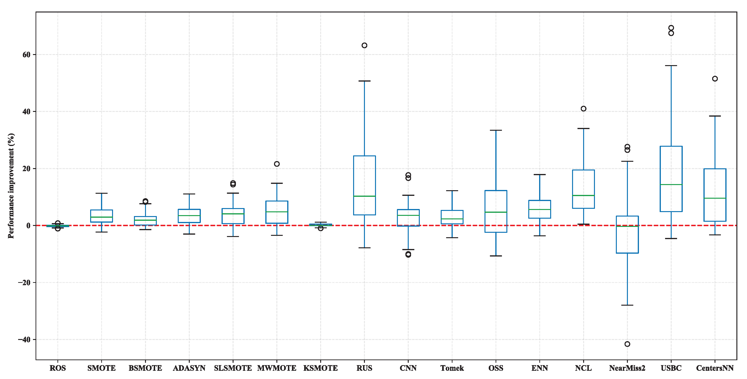
4.1. Results of RQ1
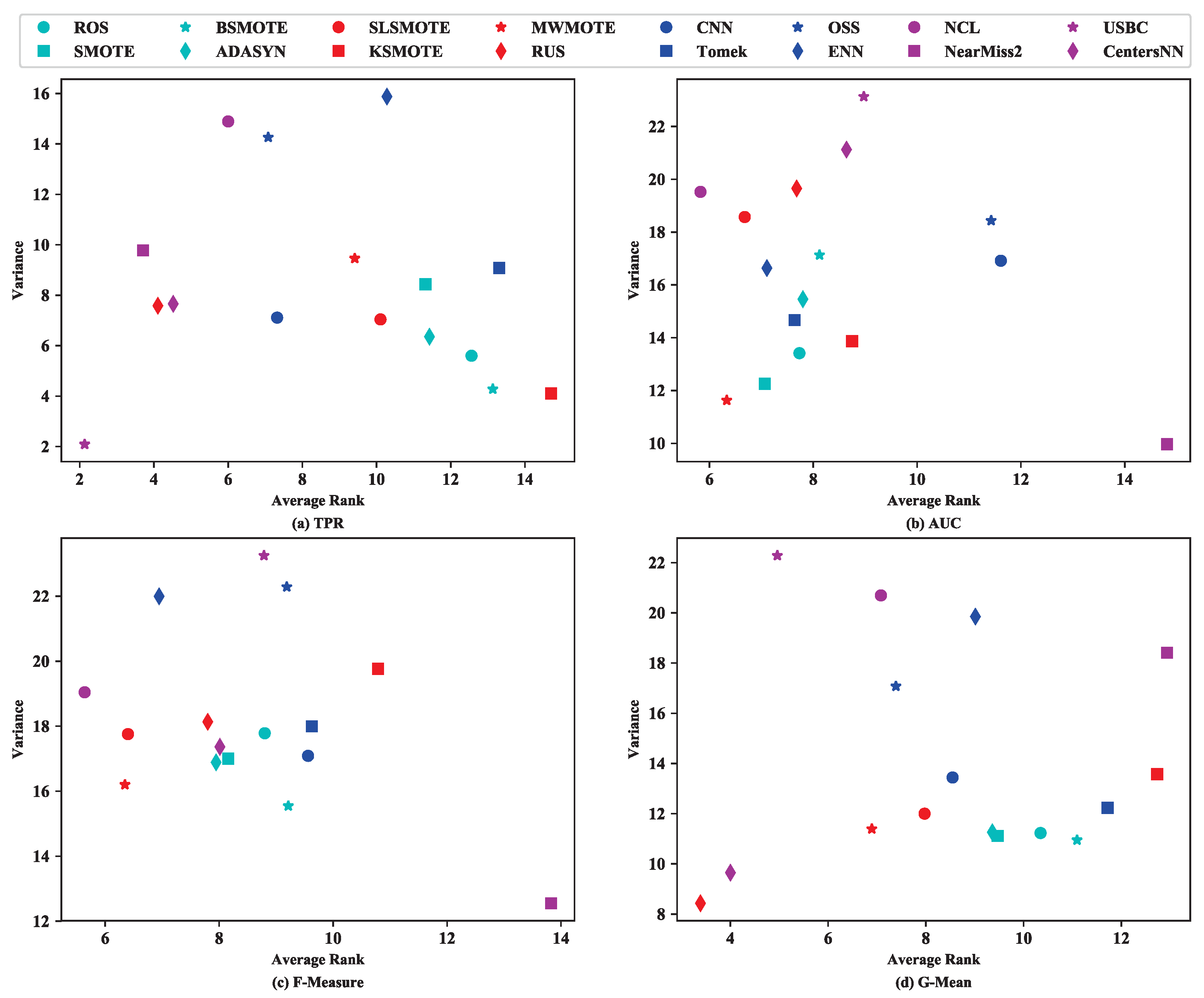
4.2. Results of RQ2
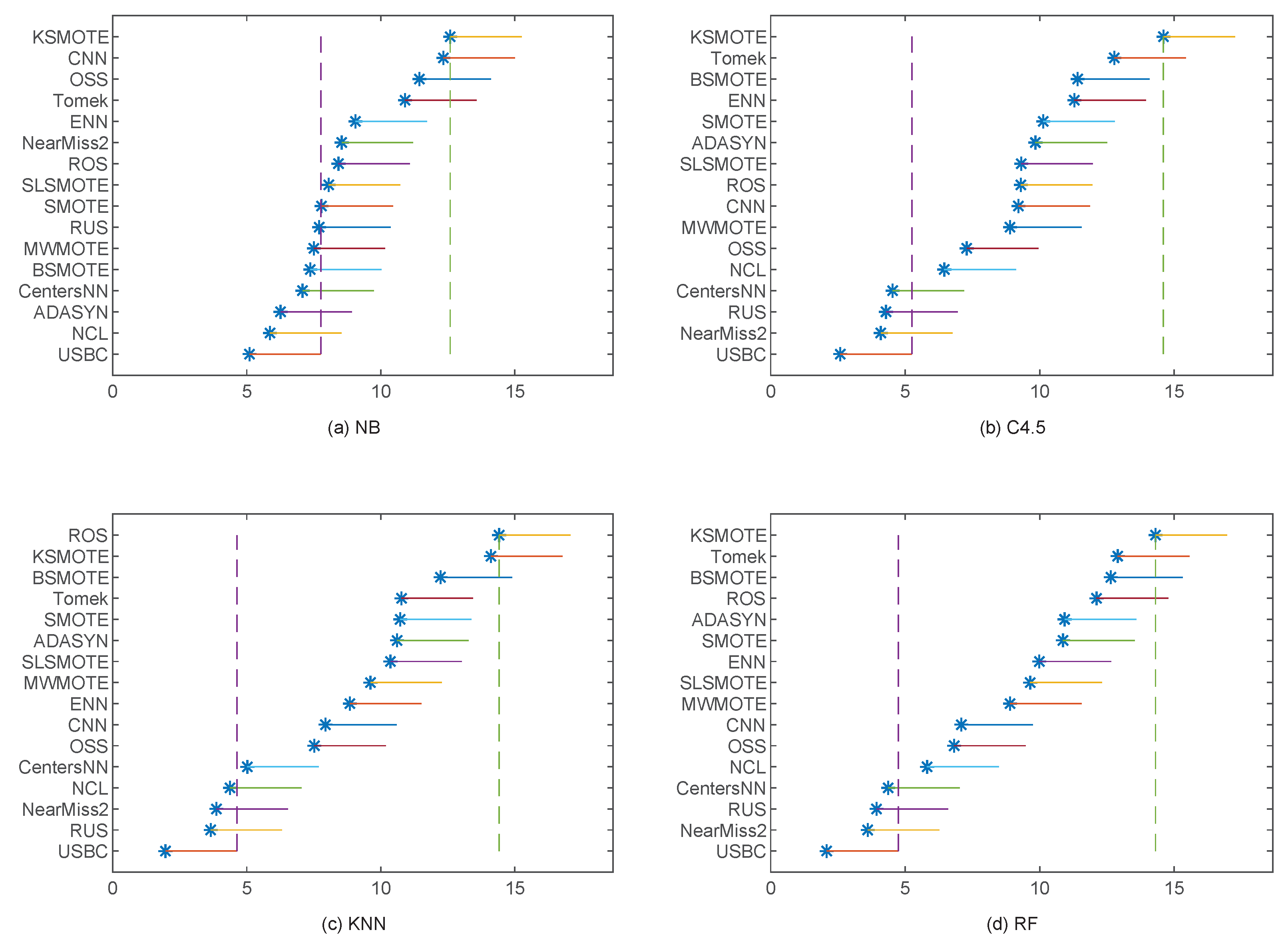
4.3. Results of RQ3
5. Conclusions
Author Contributions
Funding
Data Availability Statement
Conflicts of Interest
References
- He, H.; Garcia, E.A. Learning from Imbalanced Data. IEEE Trans. Knowl. Data Eng. 2009, 21, 1263–1284. [Google Scholar]
- Guo, G.; Li, Y.; Shang, J.; Gu, M.; Huang, Y.; Gong, B. Learning from class-imbalanced data: Review of methods and applications. Expert Syst. Appl. 2017, 73, 220–239. [Google Scholar]
- Zhu, B.; Baesens, B.; Broucke, S.K.L.M.V. An empirical comparison of techniques for the class imbalance problem in churn prediction. Inf. Sci. 2017, 408, 84–99. [Google Scholar] [CrossRef]
- Sun, Z.; Song, Q.; Zhu, X. Using coding-based ensemble learning to improve software defect prediction. IEEE Trans. Syst. Man Cybern. Part C Appl. Rev. 2012, 42, 1806–1817. [Google Scholar] [CrossRef]
- Xie, Y.; Li, S.; Wu, C.T.; Lai, Z.; Su, M. A novel hypergraph convolution network for wafer defect patterns identification based on an unbalanced dataset. J. Intell. Manuf. 2022, 1–14. [Google Scholar] [CrossRef]
- Wei, W.; Li, J.; Cao, L.; Ou, Y.; Chen, J. Effective detection of sophisticated online banking fraud on extremely imbalanced data. World Wide Web 2013, 16, 449–475. [Google Scholar] [CrossRef]
- Chawla, N.V.; Japkowicz, N.; Kotcz, A. Special issue on learning from imbalanced data sets. ACM SIGKDD Explor. Newsl. 2004, 6, 1–6. [Google Scholar] [CrossRef]
- Batista, G.E.; Prati, R.C.; Monard, M.C. A study of the behavior of several methods for balancing machine learning training data. ACM SIGKDD Explor. Newsl. 2004, 6, 20–29. [Google Scholar] [CrossRef]
- Douzas, G.; Bacao, F.; Last, F. Improving imbalanced learning through a heuristic oversampling method based on k-means and SMOTE. Inf. Sci. 2018, 465, 1–20. [Google Scholar] [CrossRef]
- López, V.; Fernández, A.; Moreno-Torres, J.G.; Herrera, F. Analysis of preprocessing vs. cost-sensitive learning for imbalanced classification. Open problems on intrinsic data characteristics. Expert Syst. Appl. 2012, 39, 6585–6608. [Google Scholar] [CrossRef]
- Yu, H.; Sun, C.; Yang, X.; Yang, W.; Shen, J.; Qi, Y. ODOC-ELM: Optimal decision outputs compensation-based extreme learning machine for classifying imbalanced data. Knowl.-Based Syst. 2016, 92, 55–70. [Google Scholar] [CrossRef]
- Galar, M.; Fernandez, A.; Barrenechea, E.; Bustince, H.; Herrera, F. A review on ensembles for the class imbalance problem: Bagging-, boosting-, and hybrid-based approaches. IEEE Trans. Syst. Man Cybern. Part C Appl. Rev. 2011, 42, 463–484. [Google Scholar] [CrossRef]
- Sun, Z.; Song, Q.; Zhu, X.; Sun, H.; Xu, B.; Zhou, Y. A novel ensemble method for classifying imbalanced data. Pattern Recognit. 2015, 48, 1623–1637. [Google Scholar] [CrossRef]
- López, V.; Fernández, A.; García, S.; Palade, V.; Herrera, F. An insight into classification with imbalanced data: Empirical results and current trends on using data intrinsic characteristics. Inf. Sci. 2013, 250, 113–141. [Google Scholar] [CrossRef]
- Estabrooks, A.; Jo, T.; Japkowicz, N. A Multiple Resampling Method for Learning from Imbalanced Data Sets. Comput. Intell. 2004, 20, 18–36. [Google Scholar] [CrossRef]
- Loyola-González, O.; Martínez-Trinidad, J.F.; Carrasco-Ochoa, J.A.; García-Borroto, M. Study of the impact of resampling methods for contrast pattern based classifiers in imbalanced databases. Neurocomputing 2016, 175, 935–947. [Google Scholar] [CrossRef]
- López, V.; Fernández, A.; Herrera, F. On the importance of the validation technique for classification with imbalanced datasets: Addressing covariate shift when data is skewed. Inf. Sci. 2014, 257, 1–13. [Google Scholar] [CrossRef]
- Chen, C.P.; Zhang, C.Y. Data-intensive applications, challenges, techniques and technologies: A survey on Big Data. Inf. Sci. 2014, 275, 314–347. [Google Scholar] [CrossRef]
- Maldonado, S.; Weber, R.; Famili, F. Feature selection for high-dimensional class-imbalanced data sets using Support Vector Machines. Inf. Sci. 2014, 286, 228–246. [Google Scholar] [CrossRef]
- Sáez, J.A.; Luengo, J.; Stefanowski, J.; Herrera, F. SMOTE–IPF: Addressing the noisy and borderline examples problem in imbalanced classification by a re-sampling method with filtering. Inf. Sci. 2015, 291, 184–203. [Google Scholar] [CrossRef]
- Krawczyk, B.; Woźniak, M.; Schaefer, G. Cost-sensitive decision tree ensembles for effective imbalanced classification. Appl. Soft Comput. 2014, 14, 554–562. [Google Scholar] [CrossRef]
- Tao, X.; Li, Q.; Guo, W.; Ren, C.; Li, C.; Liu, R.; Zou, J. Self-adaptive cost weights-based support vector machine cost-sensitive ensemble for imbalanced data classification. Inf. Sci. 2019, 487, 31–56. [Google Scholar] [CrossRef]
- Sun, J.; Lang, J.; Fujita, H.; Li, H. Imbalanced enterprise credit evaluation with DTE-SBD: Decision tree ensemble based on SMOTE and bagging with differentiated sampling rates. Inf. Sci. 2018, 425, 76–91. [Google Scholar] [CrossRef]
- Das, B.; Krishnan, N.C.; Cook, D.J. RACOG and wRACOG: Two Probabilistic Oversampling Techniques. IEEE Trans. Knowl. Data Eng. 2015, 27, 222–234. [Google Scholar] [CrossRef] [PubMed]
- Abdi, L.; Hashemi, S. To Combat Multi-Class Imbalanced Problems by Means of Over-Sampling Techniques. IEEE Trans. Knowl. Data Eng. 2016, 28, 238–251. [Google Scholar] [CrossRef]
- Yang, X.; Kuang, Q.; Zhang, W.; Zhang, G. AMDO: An Over-Sampling Technique for Multi-Class Imbalanced Problems. IEEE Trans. Knowl. Data Eng. 2018, 30, 1672–1685. [Google Scholar] [CrossRef]
- Li, L.; He, H.; Li, J. Entropy-based Sampling Approaches for Multi-class Imbalanced Problems. IEEE Trans. Knowl. Data Eng. 2019, 32, 2159–2170. [Google Scholar] [CrossRef]
- Chawla, N.V.; Bowyer, K.W.; Hall, L.O.; Kegelmeyer, W.P. SMOTE: Synthetic minority over-sampling technique. J. Artif. Intell. Res. 2002, 16, 321–357. [Google Scholar] [CrossRef]
- Fernandez, A.; Garcia, S.; Herrera, F.; Chawla, N.V. SMOTE for Learning from Imbalanced Data: Progress and Challenges, Marking the 15-year Anniversary. J. Artif. Intell. Res. 2018, 61, 863–905. [Google Scholar] [CrossRef]
- Han, H.; Wang, W.Y.; Mao, B.H. Borderline-SMOTE: A new over-sampling method in imbalanced data sets learning. In Proceedings of the International Conference on Intelligent Computing, Hefei, China, 23–26 August 2005; pp. 878–887. [Google Scholar]
- He, H.; Bai, Y.; Garcia, E.A.; Li, S. ADASYN: Adaptive synthetic sampling approach for imbalanced learning. In Proceedings of the 2008 IEEE International Joint Conference on Neural Networks, Hong Kong, China, 1–6 June 2008; pp. 1322–1328. [Google Scholar]
- Barua, S.; Islam, M.M.; Yao, X.; Murase, K. MWMOTE–majority weighted minority oversampling technique for imbalanced data set learning. IEEE Trans. Knowl. Data Eng. 2012, 26, 405–425. [Google Scholar] [CrossRef]
- Bennin, K.E.; Keung, J.; Phannachitta, P.; Monden, A.; Mensah, S. Mahakil: Diversity based oversampling approach to alleviate the class imbalance issue in software defect prediction. IEEE Trans. Softw. Eng. 2017, 44, 534–550. [Google Scholar] [CrossRef]
- Yan, Y.; Tan, M.; Xu, Y.; Cao, J.; Ng, M.; Min, H.; Wu, Q. Oversampling for Imbalanced Data via Optimal Transport. In Proceedings of the AAAI Conference on Artificial Intelligence 2019, Honolulu, HI, USA, 27 January–1 February 2019; pp. 5605–5612. [Google Scholar]
- Zhang, H.; Li, M. RWO-Sampling: A random walk over-sampling approach to imbalanced data classification. Inf. Fusion 2014, 20, 99–116. [Google Scholar] [CrossRef]
- Ofek, N.; Rokach, L.; Stern, R.; Shabtai, A. Fast-CBUS: A fast clustering-based undersampling method for addressing the class imbalance problem. Neurocomputing 2017, 243, 88–102. [Google Scholar] [CrossRef]
- Tsai, C.F.; Lin, W.C.; Hu, Y.H.; Yao, G.T. Under-sampling class imbalanced datasets by combining clustering analysis and instance selection. Inf. Sci. 2019, 477, 47–54. [Google Scholar] [CrossRef]
- Peng, M.; Zhang, Q.; Xing, X.; Gui, T.; Huang, X.; Jiang, Y.G.; Ding, K.; Chen, Z. Trainable Undersampling for Class-Imbalance Learning. In Proceedings of the AAAI Conference on Artificial Intelligence 2019, Honolulu, HI, USA, 27 January–1 February 2019; pp. 4707–4714. [Google Scholar]
- Vuttipittayamongkol, P.; Elyan, E. Neighbourhood-based undersampling approach for handling imbalanced and overlapped data. Inf. Sci. 2020, 509, 47–70. [Google Scholar] [CrossRef]
- Hart, P. The condensed nearest neighbor rule (Corresp.). IEEE Trans. Inf. Theory 1968, 14, 515–516. [Google Scholar] [CrossRef]
- Wilson, D.L. Asymptotic properties of nearest neighbor rules using edited data. IEEE Trans. Syst. Man Cybern. 1972, 2, 408–421. [Google Scholar] [CrossRef]
- Laurikkala, J. Improving identification of difficult small classes by balancing class distribution. In Proceedings of the Conference on Artificial Intelligence in Medicine in Europe 2001, Cascais, Portugal, 1–4 July 2001; pp. 63–66. [Google Scholar]
- Kubat, M.; Matwin, S. Addressing the curse of imbalanced training sets: One-sided selection. In Proceedings of the International Conference on Machine Learning 1997, Nashville, TN, USA, 8–12 July 1997; pp. 179–186. [Google Scholar]
- Tomek, I. Two modifications of CNN. IEEE Trans. Syst. Man Cybern. 1976, 6, 769–772. [Google Scholar]
- Yen, S.J.; Lee, Y.S. Cluster-based under-sampling approaches for imbalanced data distributions. Expert Syst. Appl. 2009, 36, 5718–5727. [Google Scholar] [CrossRef]
- Lin, W.C.; Tsai, C.F.; Hu, Y.H.; Jhang, J.S. Clustering-based undersampling in class-imbalanced data. Inf. Sci. 2017, 409, 17–26. [Google Scholar] [CrossRef]
- García, S.; Herrera, F. Evolutionary undersampling for classification with imbalanced datasets: Proposals and taxonomy. Evol. Comput. 2009, 17, 275–306. [Google Scholar] [CrossRef]
- Wang, N.; Zhao, X.; Jiang, Y.; Gao, Y. Iterative metric learning for imbalance data classification. In Proceedings of the 27th International Joint Conference on Artificial Intelligence 2018, Stockholm, Sweden, 13–19 July 2018; pp. 2805–2811. [Google Scholar]
- Japkowicz, N. Learning from imbalanced data sets: A comparison of various strategies. In Proceedings of the AAAI Workshop on Learning from Imbalanced Data Sets 2000, Austin, TX, USA, 31 July 2000; pp. 10–15. [Google Scholar]
- Drummond, C.; Holte, R.C. C4. 5, class imbalance, and cost sensitivity: Why under-sampling beats over-sampling. In Proceedings of the Workshop on Learning from Imbalanced Datasets II 2003, Washington, DC, USA, 1 July 2003; pp. 1–8. [Google Scholar]
- Bennin, K.E.; Keung, J.; Monden, A.; Kamei, Y.; Ubayashi, N. Investigating the effects of balanced training and testing datasets on effort-aware fault prediction models. In Proceedings of the 2016 IEEE 40th Annual Computer Software and Applications Conference, Atlanta, GA, USA, 10–14 June 2016; pp. 154–163. [Google Scholar]
- García, V.; Sánchez, J.S.; Mollineda, R.A. On the effectiveness of preprocessing methods when dealing with different levels of class imbalance. Knowl.-Based Syst. 2012, 25, 13–21. [Google Scholar] [CrossRef]
- Hulse, J.V.; Khoshgoftaar, T.M.; Napolitano, A. Experimental perspectives on learning from imbalanced data. In Proceedings of the 24th International Conference Machine Learning 2007, Corvalis, OR, USA, 20–24 June 2007; pp. 935–942. [Google Scholar]
- Bennin, K.E.; Keung, J.W.; Monden, A. On the relative value of data resampling approaches for software defect prediction. Empir. Softw. Eng. 2019, 24, 602–636. [Google Scholar] [CrossRef]
- Zhou, L. Performance of corporate bankruptcy prediction models on imbalanced dataset: The effect of sampling methods. Knowl.-Based Syst. 2013, 41, 16–25. [Google Scholar] [CrossRef]
- Napierala, K.; Stefanowski, J. Types of minority class examples and their influence on learning classifiers from imbalanced data. J. Intell. Inf. Syst. 2016, 46, 563–597. [Google Scholar] [CrossRef]
- Kamei, Y.; Monden, A.; Matsumoto, S.; Kakimoto, T.; Matsumoto, K. The effects of over and under sampling on fault-prone module detection. In Proceedings of the International Symposium on Empirical Software Engineering and Measurement 2007, Madrid, Spain, 20–21 September 2007; pp. 196–204. [Google Scholar]
- Bennin, K.E.; Keung, J.; Monden, A.; Phannachitta, P.; Mensah, S. The significant effects of data sampling approaches on software defect prioritization and classification. In Proceedings of the ACM/IEEE International Symposium on Empirical Software Engineering and Measurement 2017, Toronto, ON, Canada, 9–10 November 2017; pp. 364–373. [Google Scholar]
- Bunkhumpornpat, C.; Sinapiromsaran, K.; Lursinsap, C. Safe-level-smote: Safe-level-synthetic minority over-sampling technique for handling the class imbalanced problem. In Proceedings of the Pacific-Asia Conference on Knowledge Discovery and Data Mining 2009, Bangkok, Thailand, 27–30 April 2009; pp. 475–482. [Google Scholar]
- Barandela, R.; Valdovinos, R.M.; Sánchez, J.S.; Ferri, F.J. The imbalanced training sample problem: Under or over sampling? In Proceedings of the Joint IAPR International Workshops on Statistical Techniques in Pattern Recognition and Structural and Syntactic Pattern Recognition 2004, Lisbon, Portugal, 18–20 August 2004; pp. 806–814. [Google Scholar]
- Mani, I.; Zhang, I. kNN approach to unbalanced data distributions: A case study involving information extraction. In Proceedings of the Workshop on Learning from Imbalanced Datasets 2003, Washington, DC, USA, 1 July 2003; pp. 1–7. [Google Scholar]
- Alcalá, J.; Fernández, A.; Luengo, J.; Derrac, J.; García, S.; Sánchez, L.; Herrera, F. Keel data-mining software tool: Data set repository, integration of algorithms and experimental analysis framework. J. Mult.-Valued Log. Soft Comput. 2011, 17, 255–287. [Google Scholar]
- Dua, D.; Graff, C. UCI Machine Learning Repository. 2017. Available online: http://archive.ics.uci.edu/ml (accessed on 21 September 2023).
- Jing, X.Y.; Wu, F.; Dong, X.; Xu, B. An improved SDA based defect prediction framework for both within-project and cross-project class-imbalance problems. IEEE Trans. Softw. Eng. 2017, 43, 321–339. [Google Scholar] [CrossRef]
- Czibula, G.; Marian, Z.; Czibula, I.G. Software defect prediction using relational association rule mining. Inf. Sci. 2014, 264, 260–278. [Google Scholar] [CrossRef]
- Park, B.J.; Oh, S.K.; Pedrycz, W. The design of polynomial function-based neural network predictors for detection of software defects. Inf. Sci. 2013, 229, 40–57. [Google Scholar] [CrossRef]
- Shepperd, M.; Song, Q.; Sun, Z.; Mair, C. Data quality: Some comments on the NASA software defect datasets. IEEE Trans. Softw. Eng. 2013, 39, 1208–1215. [Google Scholar] [CrossRef]
- Jureczko, M.; Madeyski, L. Towards identifying software project clusters with regard to defect prediction. In Proceedings of the 6th International Conference on Predictive Models in Software Engineering 2010, Timisoara, Romania, 12–13 September 2010; pp. 9–18. [Google Scholar]
- Catal, C.; Diri, B. Investigating the effect of dataset size, metrics sets, and feature selection techniques on software fault prediction problem. Inf. Sci. 2009, 179, 1040–1058. [Google Scholar] [CrossRef]
- Seiffert, C.; Khoshgoftaar, T.M.; Van Hulse, J.; Folleco, A. An empirical study of the classification performance of learners on imbalanced and noisy software quality data. Inf. Sci. 2014, 259, 571–595. [Google Scholar] [CrossRef]
- Hall, M.; Frank, E.; Holmes, G.; Pfahringer, B.; Reutemann, P.; Witten, I.H. The WEKA data mining software: An update. ACM SIGKDD Explor. Newsl. 2009, 11, 10–18. [Google Scholar] [CrossRef]
- Friedman, M. The use of ranks to avoid the assumption of normality implicit in the analysis of variance. J. Am. Stat. Assoc. 1937, 32, 675–701. [Google Scholar] [CrossRef]
- Demšar, J. Statistical Comparisons of Classifiers over Multiple Data Sets. J. Mach. Learn. Res. 2006, 7, 1–30. [Google Scholar]
- Nemenyi, P. Distribution-Free Multiple Comparisons. Ph.D. Thesis, Princeton University, Princeton, NJ, USA, 1963. [Google Scholar]
- Pan, S.J.; Yang, Q. A Survey on Transfer Learning. IEEE Trans. Knowl. Data Eng. 2010, 22, 1345–1359. [Google Scholar] [CrossRef]


| ID | Data | #Min | #Total | IR | ID | Data | #Min | #Total | IR |
|---|---|---|---|---|---|---|---|---|---|
| 1 | cylinder | 228 | 540 | 1.37 | 39 | PC3 | 132 | 1073 | 7.13 |
| 2 | htru | 1639 | 17,898 | 9.92 | 40 | PC4 | 176 | 1276 | 6.25 |
| 3 | ionosphere | 126 | 351 | 1.79 | 41 | PC5 | 459 | 1679 | 2.66 |
| 4 | ozone1hr | 73 | 2536 | 33.74 | 42 | ant1.7 | 166 | 724 | 3.36 |
| 5 | ozone8hr | 160 | 2534 | 14.84 | 43 | arc | 25 | 213 | 7.52 |
| 6 | sonar | 97 | 208 | 1.14 | 44 | camel1.0 | 13 | 327 | 24.15 |
| 7 | bankruptcy1 | 271 | 7027 | 24.93 | 45 | camel1.6 | 181 | 878 | 3.85 |
| 8 | bankruptcy2 | 400 | 10,173 | 24.43 | 46 | ivy2.0 | 40 | 345 | 7.63 |
| 9 | bankruptcy3 | 495 | 10,503 | 20.22 | 47 | jedit3.2 | 90 | 268 | 1.98 |
| 10 | bankruptcy4 | 515 | 9792 | 18.01 | 48 | jedit4.2 | 48 | 363 | 6.56 |
| 11 | bankruptcy5 | 410 | 5910 | 13.41 | 49 | log4j1.1 | 37 | 109 | 1.95 |
| 12 | credit-a | 307 | 690 | 1.25 | 50 | lucene2.0 | 90 | 191 | 1.12 |
| 13 | creditC | 6636 | 30,000 | 3.52 | 51 | poi2.0 | 35 | 282 | 7.06 |
| 14 | credit-g | 300 | 1000 | 2.33 | 52 | prop1 | 1536 | 8011 | 4.22 |
| 15 | market | 5289 | 45,211 | 7.55 | 53 | prop6 | 32 | 377 | 10.78 |
| 16 | alizadeh | 87 | 303 | 2.48 | 54 | redaktor | 25 | 169 | 5.76 |
| 17 | breast-c | 85 | 286 | 2.36 | 55 | synapse1.0 | 16 | 153 | 8.56 |
| 18 | breast-w | 241 | 699 | 1.9 | 56 | synapse1.2 | 86 | 245 | 1.85 |
| 19 | coimbra | 52 | 116 | 1.23 | 57 | tomcat | 77 | 796 | 9.34 |
| 20 | colic | 136 | 368 | 1.71 | 58 | velocity1.6 | 76 | 211 | 1.78 |
| 21 | haberman | 81 | 306 | 2.78 | 59 | xalan2.4 | 110 | 694 | 5.31 |
| 22 | heart | 120 | 270 | 1.25 | 60 | xercesInit | 65 | 146 | 1.25 |
| 23 | hepatitis | 32 | 155 | 3.84 | 61 | xerces1.3 | 68 | 362 | 4.32 |
| 24 | ilpd | 167 | 583 | 2.49 | 62 | Clam_fit | 93 | 1597 | 16.17 |
| 25 | liver | 145 | 345 | 1.38 | 63 | Clam_test | 56 | 8723 | 154.77 |
| 26 | pima | 268 | 768 | 1.87 | 64 | eCos_fit | 110 | 630 | 4.73 |
| 27 | retinopathy | 540 | 1151 | 1.13 | 65 | eCos_test | 67 | 3480 | 50.94 |
| 28 | sick | 231 | 3772 | 15.33 | 66 | NetBSD_fit | 546 | 6781 | 11.42 |
| 29 | thoracic | 70 | 470 | 5.71 | 67 | NetBSD_test | 295 | 10,960 | 36.15 |
| 30 | CM1 | 42 | 327 | 6.79 | 68 | OpenBSD_fit | 275 | 1706 | 5.2 |
| 31 | JM1 | 1612 | 7720 | 3.79 | 69 | OpenBSD_test | 158 | 5964 | 36.75 |
| 32 | KC1 | 294 | 1162 | 2.95 | 70 | OpenCms_fit | 193 | 1727 | 7.95 |
| 33 | KC3 | 36 | 194 | 4.39 | 71 | OpenCms_test | 93 | 2821 | 29.33 |
| 34 | MC1 | 36 | 1847 | 50.31 | 72 | Samba_fit | 184 | 1623 | 7.82 |
| 35 | MC2 | 44 | 125 | 1.84 | 73 | Samba_test | 223 | 2559 | 10.48 |
| 36 | MW1 | 25 | 251 | 9.04 | 74 | Scilab_fit | 233 | 2636 | 10.31 |
| 37 | PC1 | 55 | 696 | 11.65 | 75 | Scilab_test | 238 | 1248 | 4.24 |
| 38 | PC2 | 16 | 734 | 44.88 |
| Predicted Positive | Predicted Negative | |
|---|---|---|
| Actual Positive | TP | FN |
| Actual Negative | FP | TN |
Disclaimer/Publisher’s Note: The statements, opinions and data contained in all publications are solely those of the individual author(s) and contributor(s) and not of MDPI and/or the editor(s). MDPI and/or the editor(s) disclaim responsibility for any injury to people or property resulting from any ideas, methods, instructions or products referred to in the content. |
© 2023 by the authors. Licensee MDPI, Basel, Switzerland. This article is an open access article distributed under the terms and conditions of the Creative Commons Attribution (CC BY) license (https://creativecommons.org/licenses/by/4.0/).
Share and Cite
Sun, Z.; Zhang, J.; Zhu, X.; Xu, D. How Far Have We Progressed in the Sampling Methods for Imbalanced Data Classification? An Empirical Study. Electronics 2023, 12, 4232. https://doi.org/10.3390/electronics12204232
Sun Z, Zhang J, Zhu X, Xu D. How Far Have We Progressed in the Sampling Methods for Imbalanced Data Classification? An Empirical Study. Electronics. 2023; 12(20):4232. https://doi.org/10.3390/electronics12204232
Chicago/Turabian StyleSun, Zhongbin, Jingqi Zhang, Xiaoyan Zhu, and Donghong Xu. 2023. "How Far Have We Progressed in the Sampling Methods for Imbalanced Data Classification? An Empirical Study" Electronics 12, no. 20: 4232. https://doi.org/10.3390/electronics12204232