Electrical Power Edge-End Interaction Modeling with Time Series Label Noise Learning

Abstract

In the context of electrical power systems, modeling the edge-end interaction involves understanding the dynamic relationship between different components and endpoints of the system. However, the time series of electrical power obtained by user terminals often suffer from low-quality issues such as missing values, numerical anomalies, and noisy labels. These issues can easily reduce the robustness of data mining results for edge-end interaction models. Therefore, this paper proposes a time–frequency noisy label classification (TF-NLC) model, which improves the robustness of edge-end interaction models in dealing with low-quality issues. Specifically, we employ two deep neural networks that are trained concurrently, utilizing both the time and frequency domains. The two networks mutually guide each other’s classification training by selecting clean labels from batches within small loss data. To further improve the robustness of the classification of time and frequency domain feature representations, we introduce a time–frequency domain consistency contrastive learning module. By classifying the selection of clean labels based on time–frequency representations for mutually guided training, TF-NLC can effectively mitigate the negative impact of noisy labels on model training. Extensive experiments on eight electrical power and ten other different realistic scenario time series datasets show that our proposed TF-NLC achieves advanced classification performance under different noisy label scenarios. Also, the ablation and visualization experiments further demonstrate the robustness of our proposed method.

1. Introduction

With the rapid development of communication technology, there is a growing demand for constructing intelligent power grid systems [1]. Designing data mining models to handle the increasing volume of electric power time series data and providing valuable insights for managing power grids has become a hot topic [2]. Existing studies primarily concentrate on designing cloud–side-end collaboration techniques for new power systems, aiming to achieve real-time analysis of massive power time series data [3]. However, when exploring cloud–side-end collaboration technology for power grids, a significant challenge emerges in utilizing the time series data acquired by the user’s intelligent terminal [4,5], which evolves over time and requires real-time data mining at the side end.

In real-life scenarios, time series data collected by power grid intelligent terminals often exhibit noticeable low-quality issues [6,7]. These issues arise due to factors such as communication failures of smart terminal equipment, sensor malfunctions, human operational errors, and adverse weather conditions, resulting in problems like missing values [8] and numerical anomalies [9] within the acquired data. Moreover, the electric power time series data frequently rely on time sliding window analysis for automatic labeling, leading to the generation of many noisy labels (incorrect labels) [10]. Directly mining and analyzing the automatically labeled power time series data using edge-end models can undermine the robustness of the models. To address the issues of missing values and numerical anomalies in power time series data, proper data preprocessing methods, such as data cleansing and missing value imputation [11,12], are essential to improve the quality of time series data. Simultaneously, robust classification methods need to be developed to handle time series noise labels, enhancing the reliability and practicality of the edge-end model for data mining analysis.

There are significant limitations in using traditional methods for massive electric power time series data. In recent years, deep-learning-based time series classification algorithms [13,14] have effectively improved the efficiency and accuracy of time series classification. However, existing deep-learning-based algorithms rely on large-scale correctly labeled data [15]. If the model is directly trained using time series containing incorrect labels, it tends to reduce the model’s robustness and produce inaccurate prediction results. To address these issues, several studies in computer vision [16,17,18] have effectively enhanced the robustness of deep learning models by designing robustness loss functions, selecting clean labeled samples, and employing techniques for correcting incorrect labels in noise label learning. However, existing studies on noise label learning for time series are still limited [10], and building a robust time series noise learning model based on existing work has not been fully explored.

Electric power time series are typical unstructured data with high-dimensional and nonlinear characteristics. Additionally, time series data exhibit traits such as temporal trends and seasonal changes [19]. To leverage the time series’ characteristics, such as temporal dependence and changing trends, related scholars [20,21] have developed various approaches to enhance the robustness of time series modeling. Dempster et al. [22,23] integrated a large number of randomly initialized convolutional kernels to learn discriminative features for time series classification. Eldele et al. [20] and Yue et al. [24] explored the ability of contrastive learning to capture the complex dynamic characteristics of time series. Woo et al. [25] and Zhang et al. [21] further improved the model’s performance on time series prediction and classification by incorporating frequency domain characteristics of time series. However, these methods mainly focus on self-supervised contrastive learning strategies or supervised learning with correct labels. In contrast, utilizing the intrinsic properties of time series (e.g., temporal dependence and frequency domain information [26]) for classification learning in the presence of noisy labels remains a challenge.

To address the aforementioned problems, we propose a robust time–frequency noisy label classification model (TF-NLC), enhancing smart grid edge-end interaction modeling. Specifically, we employ Fourier transform [27] to convert the original time series data from the time domain to frequency domain data. We simultaneously train two deep neural networks based on the time domain and frequency domain of the original time series. The time and frequency domain networks guide each other’s classification learning by leveraging the classification results from each batch of training data. To achieve this, we utilize the small-loss criterion theory for noisy labels [28] to guide the classification training of both networks. This guided training process enhances the model’s ability to resist noisy labels. Additionally, we introduce a time–frequency consistency contrastive learning module that helps alleviate the negative impact of missing values, outliers, and noisy labels in the original time series during representation learning.

Overall, the significant contributions of this paper are threefold:

• We propose a time–frequency collaborative classification learning model aimed at tackling issues related to low data quality, including problems like noisy labels and outliers, in electric power time series data. Specifically, our proposed model, in conjunction with a small loss criterion, leverages both time and frequency domain information from each sample to enhance the model’s robustness. Hence, this contributes to the enhancement of edge-end modeling for electric power time series data.
• We introduce a time–frequency contrastive learning module to capture the consistency between the time and frequency domains within each electric power time series. This helps alleviate the adverse effects of missing, anomalous values and noisy labels during model classification training. Furthermore, our model can seamlessly integrate federated learning to support edge-end modeling of electric power time series data, thereby enhancing the model’s robustness for real-world applications.
• Extensive experiments conducted on eight electric power time series datasets and ten different realistic scenario time series datasets demonstrate that our proposed TF-NLC achieves advanced classification performance in various noisy label scenarios. In addition, ablation, visualization, and edge-end interaction with federated learning experiments further indicate the robustness of different components of TF-NLC against noisy labels.

The remainder of the paper is organized into six sections, whereby a brief overview of related studies based on electrical power edge-end interaction modeling and label noise learning is given in Section 2. The proposed method is provided in Section 3. In Section 4, we present the experimental details and analysis results of the model proposed in this study using eight electric power and ten different realistic scenario time series datasets. Then, we provide a brief discussion of the main findings in Section 5. Finally, the conclusions are presented in Section 6.

2. Related Work

The study on power time series classification with noisy labels primarily encompasses two categories: power edge-end interaction modeling approaches and label noise learning approaches, both of which will be discussed in this section.

2.1. Electrical Power Edge-End Interaction Modeling

Research on cloud–side-end interaction schemes for power systems has drawn the attention of relevant scholars and has a solid research foundation [29,30]. For example, Wang et al. [31] utilized the classical paradigm of federated learning to design an authentication system for users’ power usage characteristics. Taïk et al. [32] applied federated learning to power load prediction, resulting in cloud–side-end models that can be efficiently deployed. In real power scenarios, labeling relevant electricity consumption time series samples can be affected by problems such as sensor failures, data transmission delays, or signal interruptions, resulting in the inevitable issue of noisy labels (incorrect labels) [33]. However, existing studies [34,35] focus on the efficient collaboration of cloud–side-end systems, paying less attention to the effective mining of low-quality time series data containing missing values, anomalies, and noisy labels in cloud–side-end interaction scenarios. Therefore, exploring and analyzing efficient edge-end data mining methods for the large amount of low-quality time series data generated by existing electric power smart terminals is a pressing challenge that requires urgent attention [36]. In recent years, deep-learning-based modeling techniques for time series analysis have garnered significant attention from many scholars [13,15]. These techniques leverage the powerful representation learning capabilities of deep learning models to enhance the analytical performance of downstream tasks. The above studies are primarily based on the assumption of perfectly accurate labels for the collected grid time series data. However, if these existing studies are directly applied to model edge-end interactions using grid time series data with noisy labels, they are likely to reduce the robustness of the model and lead to significant errors in classification predictions.

2.2. Label Noise Learning

In recent years, label noise learning has been extensively studied in computer vision [18], while time series label noise learning [10] is still in its early stages of development. Most of the existing label noise earning methods can be categorized into three groups: robust loss functions [37], sample selection [38,39,40], and label correction [16,17]. Among them, designing a reasonable loss function and sample selection strategy is a major hotspot in current research. The goal of loss function design [41] is to reduce the model’s susceptibility to fitting noisy labeled data. Building on this idea, Arazo et al. [42] proposed a beta-hybrid algorithm to estimate the probability of noisy labeled data, which improves the robustness of the model against noisy labeled data. Regarding clean sample selection, reasonable strategies are primarily designed based on the phenomenon that neural network models tend to fit clean labels faster than noise labels in the early stages of training. For example, Han et al. [43] designed a deep neural network model called co-teaching, which automatically selects clean labeled image data for classification training. Unlike image data, time series data consist of numerical data points recorded in chronological order, encompassing properties such as temporal dependencies and frequency domain information [25,26]. When existing label noise learning methods are directly applied to model low-quality electric power time series classification, it often leads to a degradation in the model’s classification performance.

3. Method

This section presents the specific details of the proposed methodology, divided into three subsections. Section 3.1 discusses the overall framework. Section 3.2 elaborates on the implementation process of using the time and frequency domain of time series data for classification training. Then, Section 3.3 focuses on the time–frequency contrastive learning module designed to enhance the model’s robustness in handling low-quality time series data. Lastly, Section 3.4 presents the overall training objective of the proposed model.

Table 1. Description of related abbreviations.

Symbol	Meaning
X	Original dataset
N	The size of the original dataset
T	The sequence length of time series
F	The number of variables of time series
$X_1$	Samples selected by the time domain network
$Y_1$	Labels of the samples selected by the time domain network
$X_2$	Samples selected by the frequency domain network
$Y_2$	Labels of the samples selected by the frequency domain network
$x_i$	The input of the i-th sample in the time domain network
$f_i$	The input of the i-th sample in the frequency domain network
j	The imaginary unit
$y_i$	The observed label of the i-th sample
${p^c}_i$	The network’s prediction for the i-th sample
$\mu$	The noise rate of the original dataset
$r_i$	The time domain feature representation of the i-th sample
$q_i$	The frequency domain feature representation of the i-th sample
${\mathcal{L}}_{tf-con}$	The time–frequency contrastive learning loss
${\mathcal{L}}_{ce}^{tem}$	The optimization objective of the time domain classifier
${\mathcal{L}}_{ce}^{feq}$	The optimization objective of the frequency domain classifier
${\mathcal{L}}_{total}$	The overall optimization objective
$\lambda$	The weight of ${\mathcal{L}}_{tf-con}$

displays the symbols used in this paper along with their corresponding meanings.

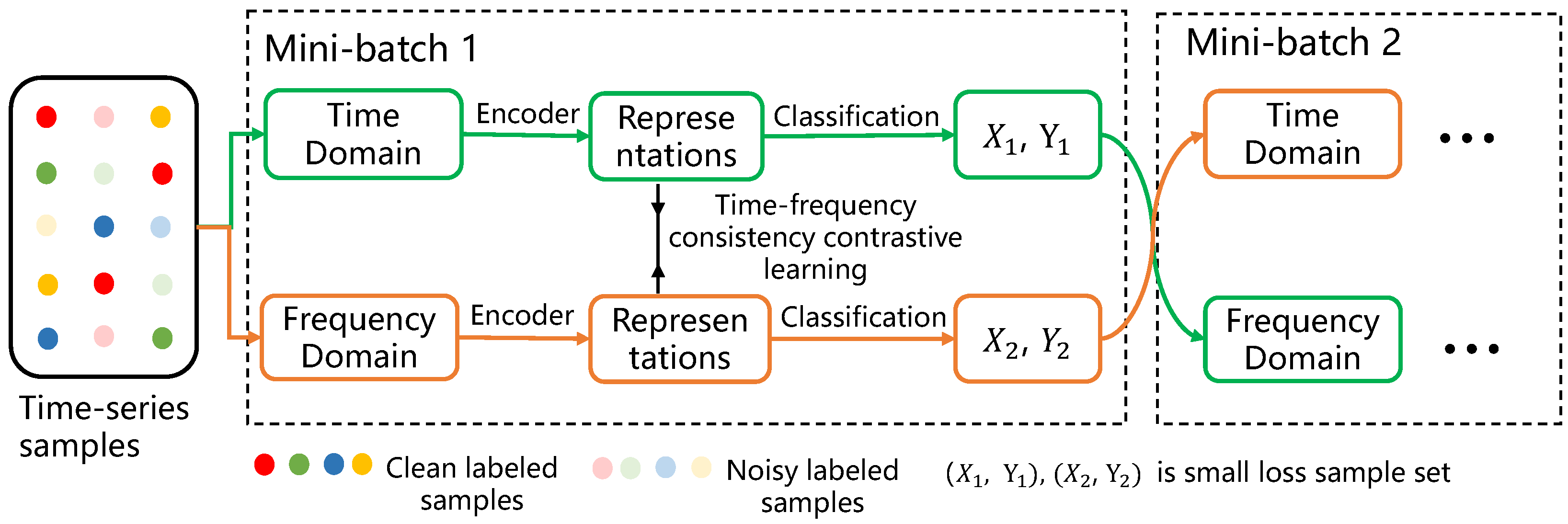
3.1. Overall Framework

In power system application scenarios, real-time electricity consumption time series data obtained from smart terminals of residential and business users suffer from issues like missing values, outliers, and noisy labels. To address the aforementioned issues, this paper first preprocesses the time series data containing missing values using the mean-imputation technique [44]. Next, we adopt a z-score normalization strategy [13] to further process raw time series. Furthermore, we design a deep learning paradigm based on the time–frequency domain of time series to handle the noise labels, thereby enhancing the model’s performance in the side-end processing and analysis of electricity power time series.

The details of the robust time–frequency noisy label classification model (TF-NLC) are shown in Figure 1. Specifically, we input the time domain data and frequency domain data of the same time series sample into two deep neural network encoders with the same structure to obtain the feature representation of the corresponding sample. Among them, the time domain data represent the original time series samples, while the frequency domain data are obtained by transforming the original time series samples via Fourier transform [27]. In the feature representation space, we introduce self-supervised contrastive learning to reduce the feature representation differences between the time and frequency domains of the same time series sample. In particular, TF-NLC aims to obtain robust feature representations by magnifying the differences in time–frequency feature representations among different time series samples. In addition, we utilize the observation labels $Y_1$ in the small loss sample set $(X_1,Y_1)$ obtained from the time domain feature representation to guide the classification training of the frequency domain feature representation, and the label $Y_2$ of the observations in the small loss sample set $(X_2,Y_2)$ obtained using the frequency domain data feature representation guides the classification training of the time domain feature representation. Utilizing the small loss samples obtained from the above time–frequency feature representations, TF-NLC synergistically cross-directs the training of each other’s classifiers, thus enhancing the model’s ability to handle noisy labels.

3.2. Time–Frequency Collaborative Classification Learning

For data collected by smart terminals, each sample can be represented as a sequence of data over a period of time. Specifically, we assume that given a set of time series $X={\left\{x_1,x_2,\dots ,x_N\right\}}_{n=1}^N$, each time series $x_n\in R^{T\times F}$, where T denotes the sequence length and F denotes the number of variables in the time series. For the problem of time series classification with noisy labels, each sample $x_i$ in the training set contains an observation label $y_i$. The goal of this paper is to use the proposed TF-NLC to automatically select which samples in the training set have observation labels that are the correct labels, and use these correct labels to guide the model in classification training, thus improving the robustness of the model against noisy labels. Although the existing noise label learning methods based on image data achieve good performance [43], they do not consider the complex dynamic change characteristics of time series. Especially when the time series data are affected by external environmental noise, some correctly labeled time series samples can easily be identified as mislabeled samples during the training process. Meanwhile, existing time series studies [21,25] demonstrate that the frequency domain information of time series is less affected by external environmental noise and can effectively reflect the seasonal trend change information of the time series samples. Inspired by the above work, this paper proposes a robust time series noisy label learning paradigm through time–frequency collaborative classification. Specifically, the fast Fourier transform (FFT) [27] is used to convert the original time series data from the time domain to the frequency domain. The FFT can be implemented using the discrete Fourier transform as follows:

$$\mathcal{F}\left[i\right]=\sum _{t=0}^{T-1}x\left[t\right]\left(cos\left(\frac{2\pi in}{T}\right)-\mathrm{j}\ast sin\left(\frac{2\pi in}{T}\right)\right),$$

(1)

where x denotes the original time series, j denotes an imaginary unit and satisfies $j^2=-1$, and $\mathcal{F}\left[i\right]$ is the frequency domain data. Using Equation (1), the original time series data can be converted into a complex form of frequency domain data $\mathcal{F}\left[i\right]$. However, the frequency domain data in the form of complex numbers cannot be directly input into the deep neural network model for training. For any complex number, this satisfies $z=a+b\ast j$, where a and b are arbitrary real numbers. In this paper, we use the real data $f_i$, which is a combination of the amplitude $\sqrt{a^2+b^2}$ and phase $arctan\frac{a}{b}$ of the original frequency domain data, as the input frequency domain data of TF-NLC.

As shown in Figure 1, the time domain data $x_i$ and frequency domain data $f_i$ of each time series sample are input to the encoder with the same structure to obtain feature representations of the same dimensional size. Based on the studies [10,13], we use a four-layer full convolutional neural network and a one-dimensional convolutional kernel as the encoder to learn the feature representations in the time–frequency domain. We then feed the acquired feature representations into a classifier consisting of a two-layer nonlinear network and obtain the classification results from the softmax function. Meanwhile, in this paper, the cross-entropy is adopted as the loss function for the classification training of the time domain and frequency domain networks as follows:

$${\mathcal{L}}_{ce}=-\frac{1}{N}\sum _{i=1}^N{y}_i^T·log\left(p_i^c\right),$$

(2)

where $p_i^c$ is equal to softmax (encoder($x_i$ or $f_i$)), and $y_i^T$ is the observed label of sample $x_i$ or $f_i$. Specifically, the time domain and frequency domain networks are trained for collaborative classification based on the proportion of $\mu$ noisy labels in the training set. In each small batch of data, we use the samples with the smallest proportion of $1-\mu$ loss values as the correctly labeled samples. Utilizing the small-loss samples selected for time–frequency collaborative classification learning, TF-NLC can leverage the consistency information between the time and frequency domains of the same time series samples to resist noisy labels, thus enhancing the robustness of the model.

3.3. Time–Frequency Contrastive Learning

The problem of model fitting with noisy labels can be alleviated by selecting observation labels with small loss samples in the time and frequency domains for collaborative classification training. However, the above strategy still does not fully leverage the time–frequency consistency information of samples from the same time series to mitigate the negative impact of numerical noise (e.g., missing values and outliers) on classification training. In recent years, contrastive learning has demonstrated unique advantages in time series modeling [21,24], which can effectively exploit the temporal dependence and frequency domain properties of time series to obtain robust representations that are beneficial for downstream tasks. To further exploit the time–frequency consistency information at the feature representation level of the time series and enhance the model’s robustness, we introduce a contrastive learning module based on the time–frequency feature representation of time series (the training process shown in Figure 1). The module is optimized with the following specific objectives:

$${\mathcal{L}}_{tf-con}=-log\frac{exp\left(r_i·q_i^{\prime }\right)}{{\sum }_{\mathrm{j}\in \mathsf{\Omega }}\left(exp\left(r_i·q_i^{\prime }\right)+1_{[j\ne \mathrm{i}]}exp\left(r_j·q_j\right)\right)},$$

(3)

where $r_i$ denotes the time domain feature representation of sample $x_i$, and $q_i^{\prime }$ denotes the frequency domain feature representation of sample $x_i$. $r_j$ and $q_j$ denote the time domain and frequency domain feature representations of the other samples in the same batch, and $\mathsf{\Omega }$ is the set of subscripts of the current batch of input time series data. Through Equation (3), TF-NLC improves the consistency of time domain and frequency domain features of samples from the same time series through a self-supervised learning strategy. The above process is unaffected by noisy labels and can somewhat counteract the negative impact of poor-quality time series information on model classification training at the feature representation level.

3.4. Overall Training Objective

Our proposed TF-NLC framework comprises two encoders with the same architecture, each corresponding to a classifier for classification training. The total training objective loss for TF-NLC is as follows:

$${\mathcal{L}}_{\mathrm{total}}={\mathcal{L}}_{ce}^{tem}+{\mathcal{L}}_{ce}^{feq}+\lambda {\mathcal{L}}_{tf-con}.$$

(4)

where ${\mathcal{L}}_{ce}^{tem}$ and ${\mathcal{L}}_{ce}^{feq}$ denote the cross-entropy loss adopted by the time and frequency domain data classifiers, respectively, and $\lambda$ is a hyperparameter used to adjust the weights of the time–frequency contrastive learning loss. By jointly optimizing the cross-entropy loss in the time and frequency domains as well as the time–frequency contrastive learning loss, the robustness of the model in dealing with low-quality time series data can be effectively improved. The algorithmic pseudocode of TF-NLC is shown in Algorithm 1.

Algorithm 1 The proposed TF-NLC framework.

Input:  time domain encoder $w_t$ and frequency domain encoder $w_f$, time domain classifier $c_t$ and frequency domain classifier $c_f$, epoch $T_{max}$, and $iteratio{n}_{max}$ within each epoch; 1: Preprocess the time series dataset using mean-imputation and normalization strategies; 2: Shuffle raw training set D with noisy labels; 3: for $t=1$ to $T_{max}$ do 4:    for $i=1$ to $iteratio{n}_{max}$ do 5:        Fetch mini-batch time data $d_t$ from D; 6:        Obtain mini-batch frequency data $d_f$ using $d_t$ and Equation (1); 7:        Obtain time domain representation r using $w_t\left(d_t\right)$; 8:        Obtain frequency domain representation q using $w_f\left(d_f\right)$; 9:        Obtain time domain clean labels $y_t$ using $c_t\left(r\right)$ via small loss criterion; 10:      Obtain frequency domain clean labels $y_f$ using $c_f\left(q\right)$ via small loss criterion; 11:      Update $w_t$ and $w_f$ using ${\mathcal{L}}_{tf-con}(r,q)$, ${\mathcal{L}}_{ce}^{tem}$ and ${\mathcal{L}}_{ce}^{feq}$ via Equation (4); 12:      Update time domain classifier $c_t$ using ${\mathcal{L}}_{ce}^{tem}(p_t,y_f)$; 13:      Update frequency domain classifier $c_f$ using ${\mathcal{L}}_{ce}^{feq}(p_f,y_t)$; 14:    end for 15: end for Output:  $w_t$, $w_f$, $c_t$ and $c_f$.

4. Experiments

In this section, we compare the proposed method with other label noise learning methods. Section 4.1 describes the experimental settings. Section 4.2 presents the comparison results of all methods conducted on a single device. Section 4.3 demonstrates the results of ablation experiments conducted on a single device. In Section 4.4, we conduct a loss analysis. Finally, in Section 4.5, we integrate our proposed method in the scenario of electrical power edge-end interaction leveraging federated learning algorithms and show the classification results.

4.1. Experiment Settings

4.1.1. Datasets

We conduct experiments on 10 public datasets, including 8 UCR datasets [45] and 2 UEA datasets [46].

Table 2. In order, the following are eight UCR datasets, two UEA datasets, and eight electric load datasets that we collected.

Dataset	#Class	#Instances	#Dimensions	#Length	Type
ArrowHead	3	211	1	251	IMAGE
CBF	3	930	1	128	SIMULATED
FaceFour	4	112	1	350	IMAGE
MelbournePedestrian	10	3650	1	24	Traffic
OSULeaf	6	442	1	427	IMAGE
Plane	7	210	1	144	SENSOR
Symbols	6	1020	1	398	IMAGE
Trace	4	200	1	275	SENSOR
Epilepsy	4	275	3	207	HAR
NATOPS	6	360	24	51	HAR
C1P1	2	63	1	96	SENSOR
C1P2	2	97	1	96	SENSOR
C1P3	2	139	1	96	SENSOR
C2P1	2	220	1	96	SENSOR
C2P2	2	98	1	96	SENSOR
C3P1	2	412	1	96	SENSOR
C3P2	2	42	1	96	SENSOR
C3P3	2	420	1	96	SENSOR

gives detailed feature information of these datasets. The UCR dataset and the UEA dataset are widely used to verify the performance of the model in time series classification tasks. The 10 datasets used in this paper remain the same as SREA [10], among which the FaceFour dataset has the smallest sample size, containing 112 samples; the MelbournePedestrian dataset has the largest sample size, including 3650 samples.

C1P{}, C2{}, and C3{} are the active electrical load data of a semiconductor materials company, an electrical appliance manufacturing company, and a technology company, respectively. In these datasets, P{i} represents the data collected at the i-th measurement point. The time series of each dataset is obtained by sampling at a frequency of 15 min per day, resulting in 96 data points for each time series. When these sequences are automatically labeled by the machine, there may be a large number of noisy labels. Therefore, we had professionals carefully correct them. Each dataset was categorized into two classes: regular electricity consumption behavior and abnormal electricity consumption behavior. The latter includes instances where customers deviate from conventional electricity usage patterns due to changing demands or sensor malfunctions. In Figure 2, the left plot shows the blue curve representing a time series in C1P1 that is labeled as normal electricity consumption behavior. On the right plot, the red curve represents a series in C1P1 that is labeled as abnormal electricity consumption behavior (notably around 9 o’clock, where there is an abnormal fluctuation in the sensor readings).

We consider three kinds of noise labels in the dataset: symmetric noise (Sym), asymmetric noise (Asym), and instance-dependent noise (IDN), and we note the noise rate as $\eta$. For symmetric noise, the probability of each sample in the dataset being mislabeled as another class is $\frac{\eta }{c-1}$ (where c is the number of labels). The asymmetric noise considered in this paper is paired noise: class A ⟶ class B, class B ⟶ class C, class C ⟶ class A, where the probability of labels flipping to incorrect ones is $\eta$. For instance-dependent noise (IDN), we corrupt labels as [47] do. The probability of each sample being mislabeled depends on the instance itself. The more similar instances from two categories are, the more likely it is that the labels of these two instances will be confused. In order to avoid unstable training as much as possible and unfair comparison of different methods, we will report the average results of all methods on these 10 datasets.

4.1.2. Evaluation Metrics

Since the number of samples of different categories in each dataset is usually uneven, using the traditional classification accuracy as an evaluation index is often disturbed by the class imbalance problem, resulting in the model evaluation not reflecting the true level. This paper adopts a more reasonable evaluation index, the weighted F1 score, as shown in Equation (5):

$$weighted\_F1=\sum _{i=1}^C{\tau }_i·\frac{2·{precision}_i·{recall}_i}{{precision}_i+{recall}_i},$$

(5)

where C represents the total number of categories in the dataset, and ${\tau }_i$ represents the proportion of Class i.

The weighted F1 score can effectively avoid the unreasonable evaluation caused by the class imbalance problem. As the test results of the model in the last few training rounds are not always stable, we report the test results of the last 10 training rounds as the final results in order to avoid unstable fluctuation. We use Equation (6) to evaluate the classification performance of the model in the dataset containing noisy labels:

$$Avw\_F1=\sum _{i=epochs-9}^{T_{max}}weighted\_F{1}_i/10.$$

(6)

where $T_{max}$ represents the number of training rounds, and $weighted\_F{1}_i$ represents the weighted F1 score obtained by evaluating the model on the test set after training i rounds.

4.1.3. Architecture

We use a four-layer full convolutional neural network with four convolution blocks and a one-dimensional convolution kernel as the encoder. Each convolution block is composed of a convolution layer, batch normalization and ReLU activation function, and dropout. Dropout at the back of the block is applied to improve the representation ability of the neural network. The dropout rate is set to 0.2, and the number of convolution kernels in the four convolution blocks is consistent with the setting of SREA [10] for a fair comparison. The dimensionality of the embedding features output from the 1D convolution kernel is 32. Then, the features are input into a nonlinear classifier, where the classifier has 128 hidden neurons.

It should be noted that the method proposed in this paper needs to encode the time series data in the time domain and the frequency domain separately, so two separate encoders with the above structure are adopted. It is different from co-teaching, which uses two differently initialized encoders that both encode the time series in the time domain.

4.1.4. Baselines

Different from the data types that this paper focuses on, current label noise learning methods primarily concentrate on image data, and many of these methods employ diverse architectures. To ensure fair comparisons, all the methods adopt the same framework mentioned in Section 4.1.3. The baselines we compared are as follows:

• Vanilla: Only the basic network framework is adopted, without using any label noise learning techniques.
• Co-teaching [43]: This method trains two differently initialized networks at the same time, and each network selects small-loss samples to guide the other network to update parameters.
• Mixup-BMM [42]: Mixup-BMM uses the beta mixture model to fit the loss distribution of the data, and combines bootstrapping and mixup for loss correction.
• SIGUA [40]: SIGUA selects clean samples and noisy samples from the training set through the small-loss criterion, uses the loss of clean samples to perform gradient descent updates, and uses the loss of noisy samples to perform gradient ascent updates.
• DivideMix [17]: DivideMix selects clean samples to form a labeled sample set, selects noisy samples to form an unlabeled sample set, and then uses these two sets combined with semisupervised learning techniques to train the network.
• SREA [10]: SREA mainly proposes an effective self-supervised learning paradigm to correct labels for mislabeled samples and uses autoencoders to help the model obtain robust representations of time series.
• Sel-CL [39]: Sel-CL selects trusted samples from the training set to construct trusted sample pairs for supervised contrastive learning, improves the accuracy of sample selection, and forms a positive cycle with the construction of trusted sample pairs.

Like co-teaching and SIGUA, TF-NLC also assumes that the noise rate is known.

4.1.5. Implementation Details

The max epochs ($T_{max})$ for all methods is set to 200. We use the Adam optimizer, the weight decay rate is set to ${10}^{-4}$, and the initial learning rate is set to ${10}^{-3}$ and halved every 60 epochs. We combine the original training set and test set, and then perform fivefold cross-validation in which four folds of data are used for training and the remaining is used for testing. We set the batch size as $min(dataset\_size/10,128)$ (where $dataset\_size$ represents the total number of samples in the training set). As mentioned above, the average value of the test results in the last 10 epochs is reported. Furthermore, due to the adoption of fivefold cross-validation, each method requires five evaluations, and the final test result is based on the average of these five evaluations. Additionally, due to the adoption of fivefold cross-validation, each method requires evaluation five times, and the final test result is obtained by averaging these five evaluations. Moreover, as mentioned earlier, deep neural networks exhibit memory effects, causing the model to focus on learning patterns from clean data in the early phase. It often requires some time to warm up. Therefore, we set the starting epoch for contrastive learning at the 30th epoch to avoid prematurely interfering with the model’s adaptation to clean data patterns in both the time and frequency domains.

4.2. Experiment Results

Table 3. Comparison with baseline methods in Avw_F1 on eight UCR datasets and two UEA datasets. The best results are in bold. The second-best results are underlined.

		Vanilla	SIGUA	Co-Teaching	BMM	Dividemix	Sel-CL	SREA	TF-NLC
Clean	0	0.947	0.942	0.954	0.872	0.462	0.832	0.961	0.956
Sym	15%	0.863	0.868	0.906	0.879	0.591	0.793	0.924	0.921
	30%	0.748	0.777	0.847	0.822	0.605	0.768	0.858	0.882
	45%	0.579	0.655	0.699	0.716	0.53	0.722	0.706	0.768
	60%	0.397	0.5	0.509	0.559	0.41	0.637	0.546	0.585
Asym	10%	0.897	0.899	0.931	0.882	0.572	0.804	0.93	0.932
	20%	0.821	0.838	0.892	0.848	0.572	0.795	0.881	0.898
	30%	0.734	0.776	0.812	0.8	0.568	0.763	0.806	0.841
	40%	0.594	0.648	0.723	0.696	0.541	0.679	0.688	0.723
IDN	30%	0.69	0.743	0.781	0.78	0.577	0.765	0.802	0.828
	40%	0.609	0.658	0.71	0.703	0.546	0.735	0.72	0.759

compares our method with others on eight UCR and two UEA datasets in Avw_F1. It indicates that our method achieves suboptimal results on clean datasets and datasets with 15% and 60% symmetric noise but outperforms other methods in all other noise. Particularly, our method exhibits a significant advantage under 45% symmetric noise, surpassing the suboptimal result by 0.046 in Avw_F1. Additionally, our method and co-teaching jointly achieve the best results on datasets with 40% asymmetric noise. However, when datasets contain higher (60%) symmetric noise, our method performs poorly, obtaining a value inferior to that of the Sel-CL method by 0.52. Overall, our method achieves state-of-the-art (SOTA) results.

Table 4. Comparison with baseline methods in the average rank on eight UCR datasets and two UEA datasets. The best results are in bold. The second-best results are underlined.

		Vanilla	SIGUA	Co-Teaching	BMM	Dividemix	Sel-CL	SREA	TF-NLC
Clean	0	3.4	4.8	3	6	8	5.8	2.1	3
Sym	15%	5.8	5.6	3.2	3.9	7.3	5.3	2.4	2.6
	30%	6	5.8	3.7	4	6.8	4.5	2.8	2.4
	45%	7	5.2	4.1	3.5	6.3	4.1	3.5	2.3
	60%	7.1	4.9	5.1	3.2	6.3	3	3.5	2.9
Asym	10%	5.2	4.9	2.6	4.8	7.4	5.2	2.9	3
	20%	5.9	5.4	3	4.6	7.1	4.3	3	2.7
	30%	5.8	5.3	3.6	4.2	6.7	4.5	3.2	2.7
	40%	6.5	5.6	2.8	4.1	6.2	4.4	3.8	2.6
IDN	30%	6.7	5.4	4	3.8	6.3	3.8	3.2	2.9
	40%	6.6	6.2	3.6	3.9	5.9	3.6	3.4	2.8

presents the average rank compared with other methods. Our method outperforms the suboptimal method (SREA) on average by 0.355 and achieves suboptimal results on clean datasets (3) as well as datasets containing 15% symmetric noise (2.6). It achieves optimal results in scenarios except for 10% asymmetric noise. The highest performance reached is 2.3. Furthermore, our method maintains an average rank between 2 and 3 across all noise levels, indicating the stability of our approach in consistently delivering optimal performance. This result aligns with the findings presented in Table 3. We also note that although SREA displayed suboptimal results in Table 4, it did not consistently demonstrate suboptimal performance in Table 3. This can be attributed to the lack of stability in SREA’s performance and its relatively weaker classification abilities on some datasets. Additionally, it is worth noting that in Table 3, our method is inferior to Sel-CL on datasets with 60% symmetric noise, but Table 4 shows that our method is superior to Sel-CL in the average rank. The reason for this discrepancy is that, among the selected 10 datasets, Sel-CL excels at classifying a few datasets with higher levels of noise, while our method demonstrates stronger overall adaptability to noisy labels.

We compared the classification results of TF-NLC with other methods on the electricity datasets we collected. Since all electricity datasets contain two categories, we only consider symmetric noise and instance-dependent noise types in this analysis. The results are shown in

Table 5. Comparison with baseline methods in Avw_F1 on our electricity datasets. The best results are in bold. The second-best results are underlined.

		Vanilla	SIGUA	Co-Teaching	BMM	Dividemix	Sel-CL	SREA	TF-NLC
Clean	0	0.870	0.863	0.871	0.786	0.527	0.869	0.839	0.876
Sym	10%	0.830	0.825	0.832	0.763	0.569	0.828	0.809	0.846
	20%	0.780	0.800	0.806	0.748	0.541	0.762	0.772	0.813
	30%	0.744	0.721	0.734	0.682	0.600	0.720	0.718	0.756
	40%	0.629	0.621	0.609	0.611	0.591	0.679	0.620	0.647
IDN	30%	0.726	0.734	0.727	0.718	0.586	0.719	0.701	0.759
	40%	0.653	0.595	0.621	0.661	0.498	0.707	0.632	0.662

and the evaluation metric used is Avw_F1. We observed that many methods performed even worse than Vanilla, such as SIGUA, BMM, and Dividemix. Our method, on the other hand, only performed worse than Sel-CL in the case of high noise levels (40%) while outperforming other methods significantly in all other scenarios (with an average improvement of 0.013 over suboptimal results and 0.018 over Vanilla). This suggests that our method’s utilization of both temporal and frequency information plays a significant role in filtering out noisy samples in the collected electricity dataset. It further demonstrates that when addressing noisy label issues in time series, incorporating the frequency information can enhance the identification of noisy samples.

4.3. Ablation Analysis

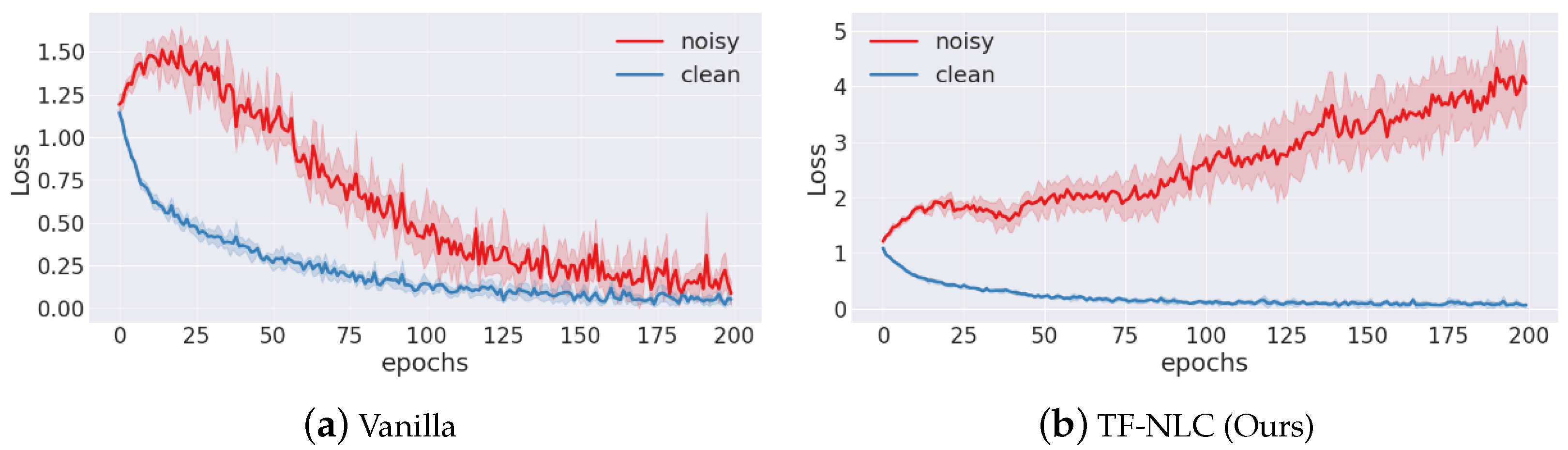
In order to further verify the effectiveness of each component of the method proposed in this paper, we conducted the following ablation experiments under the setting of 30% symmetric noise: w/o Sel. indicates TF-NLC without the process of sample selection; w/o $L_{tf-con}$ denotes TF-NLC without contrastive learning. FF represents the encoders of the dual network encoding time series in the frequency domain, while TT signifies the encoders of the dual network encoding time series in the time domain.

Table 6. The ablation experiment under the 30% symmetric noise setting in Avw_F1. w/o Sel. indicates TF-NLC without the process of sample selection; w/o $L_{tf-con}$ denotes TF-NLC without contrastive learning. FF represents the encoders of the dual network encoding time series in the frequency domain, while TT signifies the encoders of the dual network encoding time series in the time domain. Bold indicates the best results, and underline represents the second-best results.

	Vanilla	w/o Sel.	w/o ${\mathit{L}}_{\mathit{tf}-\mathit{con}}$	FF	TT	TF-NLC
ArrowHead	0.773	0.826	0.893	0.853	0.843	0.902
CBF	0.774	0.794	0.779	0.545	0.869	0.803
FaceFour	0.785	0.877	0.877	0.840	0.875	0.898
MelbournePedestrian	0.768	0.796	0.847	0.720	0.875	0.851
OSULeaf	0.670	0.754	0.773	0.652	0.806	0.807
Plane	0.771	0.829	0.947	0.958	0.944	0.956
Symbols	0.768	0.884	0.966	0.920	0.971	0.970
Trace	0.720	0.906	0.966	0.954	0.928	0.968
Epilepsy	0.760	0.904	0.895	0.837	0.838	0.902
NATOPS	0.672	0.731	0.737	0.640	0.713	0.767
Average	0.746	0.830	0.868	0.792	0.866	0.882

shows the results of the ablation experiments. In the presence of 30% symmetric noise, w/o Sel. outperforms Vanilla by an average of 0.84 across all datasets, indicating that the model that learns time series in the frequency domain also has the ability to fight against noisy labels even without using sample selection. In addition, in order to illustrate that the model plays a key role in the mutual guidance of the time domain and frequency domain of the time series to combat noisy labels, we compare the following three methods: FF, TT, and TF. Both TT and FF have lower average results (0.792 and 0.866, respectively) than TF-NLC (0.886). It demonstrates that networks that solely consider the time domain or frequency domain information of time series have significant biases in learning the data distribution. However, by working in the time and frequency domains, respectively, and guiding each other, these networks can reduce the accumulation of such biases. Additionally, we observe that the average performance of FF is lower than that of TT by 0.74, which indicates that networks learning only from the frequency domain of time series exhibit significantly weaker classification capabilities in combating noisy labels compared to networks learning from the time domain. We believe this is because using fast Fourier transform to extract frequency information from the original data results in the loss of crucial details, such as the inherent time dependencies, variation rates, peak values, and other characteristics of the time series. These features are often vital for neural networks to effectively perform time series classification tasks.

Figure 3 is a t-SNE visualization of the data features learned by the encoder of FF, TT, and TF-NLC on the Epilepsy dataset containing 30% symmetric noise. It can be found that, compared to the dual network working in the separate time domain or frequency domain, TF-NLC can learn a more robust representation (the feature representation in Figure 3c/Figure 3d is more compact than that in Figure 3a/Figure 3b). Although some noisy samples are not accurately classified, it still illustrates the effectiveness of combining time domain and frequency domain networks in combating time series noisy labels.

4.4. Loss Analysis

Figure 4a,b show the average loss of clean samples and noise samples in the training process of Vanilla and TF-NLC, respectively. It can be found that in the early stage of training, the average loss of clean samples and noise samples of both methods maintains a gap, which is in line with the widely recognized memory effect of deep neural networks [48]. Since Vanilla does not take the means against noisy labels, the loss of noisy samples gradually converges with training, resulting in a smaller difference from the average loss of clean samples. The proposed method in this paper mitigates the impact of noisy labels by employing sample selection. Furthermore, through the collaboration of two networks working in the time domain and frequency domain, it reduces the bias accumulation of sample selection. As a result, the average loss of noisy samples diverges further during training, which facilitates the selection of clean samples based on the small-loss criterion during the phase of sample selection.

4.5. Edge-End Interaction

Given the ability of federated learning to be deployed within edge-end systems for model training, this section explores the integration of the proposed method with the classical federated learning algorithm, FedAVG [49], to simulate real-world applications in electrical power edge-end systems. To be more convincing, we conducted experiments not only on the collected set of 8 electric load datasets but also on an additional 10 UCR and UEA datasets, uniformly introducing 30% symmetric label noise. The experimental settings are outlined below: considering the relatively small dataset size, we set the number of edge devices as two, each employing an independently and identically distributed training set. The local training epochs for edge devices are set to 10. The global training rounds is 20, and the batch size is either 6 or one-tenth of the training set size. Other hyperparameters are the same as Section 4.1.5.

To assess the practicality of deploying our approach within edge-end systems, we compare the following two models: TF-NLC-FedAVG (the proposed method combined with classical federated learning FedAVG) and Vanilla-FedAVG (Vanilla combined with FedAVG).

Table 7. Comparison of Vanilla-FedAVG and TF-NLC on 10 UCR and UEA datasets with 30% symmetric noise. The best results are in bold.

	Accuracy		Avw_F1
	Vanilla-FedAVG	TF-NLC-FedAVG	Vanilla-FedAVG	TF-NLC-FedAVG
ArrowHead	0.399	0.573	0.312	0.535
CBF	0.807	0.838	0.789	0.822
FaceFour	0.535	0.642	0.503	0.619
MelbournePedestrian	0.285	0.485	0.233	0.456
OSULeaf	0.285	0.468	0.202	0.426
Plane	0.791	0.891	0.784	0.863
Symbols	0.463	0.705	0.395	0.657
Trace	0.765	0.795	0.729	0.746
Epilepsy	0.749	0.782	0.748	0.774
NATOPS	0.739	0.764	0.735	0.752
Average	0.582	0.694	0.543	0.665

and

Table 8. Comparison of Vanilla-FedAVG and TF-NLC on eight electric load datasets with 30% symmetric noise. The best results are in bold.

	Accuracy		Avw_F1
	Vanilla-FedAVG	TF-NLC-FedAVG	Vanilla-FedAVG	TF-NLC-FedAVG
C1P1	0.633	0.685	0.606	0.652
C1P2	0.630	0.715	0.607	0.676
C1P3	0.684	0.749	0.685	0.747
C2P1	0.832	0.906	0.830	0.900
C2P2	0.763	0.814	0.758	0.812
C3P1	0.757	0.803	0.769	0.801
C3P2	0.861	0.950	0.834	0.950
C3P3	0.850	0.855	0.845	0.849
Average	0.751	0.809	0.742	0.798

present the experimental results. Table 7 presents the experimental results on 10 UCR and UEA datasets. TF-NLC-FedAVG outperforms Vanilla-FedAVG with an average accuracy improvement of 0.112. The largest gap between the two methods is observed on the Symbols dataset, where the difference reaches 0.242. In terms of Avw_F1, TF-NLC-FedAVG surpasses Vanilla-FedAVG by an average of 0.122, and, once again, the largest gap is observed on the Symbols dataset, with a difference of 0.262. Table 8 displays the results on eight electricity datasets. TF-NLC-FedAVG achieves a higher average accuracy of 0.58 compared to Vanilla-FedAVG. Regarding the average Avw_F1, there is a difference of 0.56 between the two methods. It can be observed that TF-NLC-FedAVG consistently performs better across all datasets. It further illustrates that the deployment of our proposed method within edge-end systems effectively mitigates the degradation of model generalization caused by noisy labels.

Additionally, we observed that the performance of both models on the 10 UCR and UEA datasets with 30% symmetric noise does not surpass the results shown in Table 3 (experiments were conducted on one single device). The reason is that datasets in Table 3 are multiclass. For instance, MelbournePedestrian comprises 10 classes with relatively short sequences. Dividing the dataset into two subsets for training on separate edge devices significantly increases the difficulty, coupled with the impact of a considerable amount of noisy labels. As a result, the model’s generalization performance is compromised. Conversely, in the case of the eight electric load datasets with 30% symmetric noise, TF-NLC-FedAVG outperforms TF-NLC in Table 3. This can be attributed to the longer sequence lengths and fewer categories within these electrical load datasets, making it easier for the model to capture data patterns. Furthermore, TF-NLC-FedAVG demonstrates improved performance in the presence of noise, leveraging TF-NLC to combat noisy labels.

5. Discussion

Noisy labels of time series exist in various domains, including healthcare, transportation, and power systems [33]. Data in these domains often possess real-time characteristics, complexity, and high dimensionality, making them susceptible to noisy labels due to environment, equipment, or human factors. While current label noise learning methods predominantly focus on computer vision, there has been limited attention paid to addressing noisy labels in the domain of time series data.

To address it, this paper proposes a novel label noise learning method that utilizes dual networks trained on temporal and frequency domains, mutually guiding each other. This method effectively handles noisy labels, thereby enhancing the accuracy and stability of model training and application. In the context of power edge-end systems, automatic data labeling is prone to noisy labels. By applying the TF-NLC method to the client side of power edge-end systems and integrating it with federated learning, a robust classification algorithm is provided for power companies. By classifying power data into normal and abnormal power consumption behaviors, the timely detection of potential issues is facilitated, allowing for the optimization of energy consumption and equipment operation. In terms of load balancing and resource allocation, our method offers targeted decision support for power companies, facilitating efficient and stable operation of power systems.

As well as providing a robust classification algorithm for the client side in cloud–edge systems, it is worth noting that our method offers an effective solution to address time series noisy labels and contribute to the development of related domains. Yet, there is still room for improvement. Future research can explore the integration of temporal and spectral information technologies and label correction methods to improve the accuracy and robustness of label noise learning methods for time series. We will also consider integrating more efficient federated learning methods to improve the reliability of cloud–edge systems.

6. Conclusions

To address the low-quality problem of missing values, outliers, and noisy labels in electric power time series data mining analysis, this paper proposes a robust time–frequency noisy label classification model (TF-NLC) that is capable of incorporating federated learning for power edge-end interaction modeling. Specifically, our proposed TF-NLC integrates the small loss criterion theory to exploit the category consistency between time and frequency domain information for each sample, addressing the low-quality aspects of power time series. Additionally, TF-NLC introduces a time–frequency self-supervised contrastive learning module to mitigate the adverse effects of missing values, outliers, and noisy labels on the classification of time–frequency feature representations. Across eight electric power time series datasets and ten UCR/UEA time series datasets, encompassing scenarios with missing and outlier values in various real-world settings, TF-NLC significantly outperforms comparison methods, such as co-teaching [43] and SREA [10], in classification accuracy under symmetric, asymmetric, and instance noise labeling settings. Furthermore, TF-NLC, when combined with federated learning, achieves an average classification accuracy at least 4% higher than the benchmark method across eight energy datasets in side-end interaction modeling experiments. This further demonstrates TF-NLC’s robustness in handling low-quality energy time series data. In the future, we plan to explore time series pretraining modeling techniques to further enhance the robustness of electrical power side-end modeling.

References

1. Yang, H.F.; Chen, Y.P.P. Hybrid deep learning and empirical mode decomposition model for time series applications. Expert Syst. Appl. 2019, 120, 128–138. [Google Scholar] [CrossRef]
2. Mollik, M.S.; Hannan, M.A.; Reza, M.S.; Abd Rahman, M.S.; Lipu, M.S.H.; Ker, P.J.; Mansor, M.; Muttaqi, K.M. The Advancement of Solid-State Transformer Technology and Its Operation and Control with Power Grids: A Review. Electronics 2022, 11, 2648. [Google Scholar] [CrossRef]
3. Zhang, H.; Bosch, J.; Olsson, H.H. Real-time end-to-end federated learning: An automotive case study. In Proceedings of the 2021 IEEE 45th Annual Computers, Software, and Applications Conference (COMPSAC), Madrid, Spain, 12–16 July 2021; pp. 459–468. [Google Scholar]
4. Wu, Q.; Chen, X.; Zhou, Z.; Zhang, J. Fedhome: Cloud-edge based personalized federated learning for in-home health monitoring. IEEE Trans. Mob. Comput. 2020, 21, 2818–2832. [Google Scholar] [CrossRef]
5. Chen, R.; Cheng, Q.; Zhang, X. Power Distribution IoT Tasks Online Scheduling Algorithm Based on Cloud-Edge Dependent Microservice. Appl. Sci. 2023, 13, 4481. [Google Scholar] [CrossRef]
6. Teimoori, Z.; Yassine, A.; Hossain, M.S. A secure cloudlet-based charging station recommendation for electric vehicles empowered by federated learning. IEEE Trans. Ind. Inform. 2022, 18, 6464–6473. [Google Scholar] [CrossRef]
7. Fekri, M.N.; Grolinger, K.; Mir, S. Distributed load forecasting using smart meter data: Federated learning with Recurrent Neural Networks. Int. J. Electr. Power Energy Syst. 2022, 137, 107669. [Google Scholar] [CrossRef]
8. Liu, Z.; Chen, C.; Ma, Q. Category-aware optimal transport for incomplete data classification. Inf. Sci. 2023, 634, 443–476. [Google Scholar] [CrossRef]
9. Sater, R.A.; Hamza, A.B. A federated learning approach to anomaly detection in smart buildings. ACM Trans. Internet Things 2021, 2, 1–23. [Google Scholar] [CrossRef]
10. Castellani, A.; Schmitt, S.; Hammer, B. Estimating the electrical power output of industrial devices with end-to-end time-series classification in the presence of label noise. In Proceedings of the Joint European Conference on Machine Learning and Knowledge Discovery in Databases, Online, 13–17 September 2021; pp. 469–484. [Google Scholar]
11. Little, R.J.; Rubin, D.B. Statistical Analysis with Missing Data; John Wiley & Sons: Hoboken, NJ, USA, 2019. [Google Scholar]
12. Huang, M.; Liu, Z.; Tao, Y. Mechanical fault diagnosis and prediction in IoT based on multi-source sensing data fusion. Simul. Model. Pract. Theory 2020, 102, 101981. [Google Scholar] [CrossRef]
13. Ismail Fawaz, H.; Forestier, G.; Weber, J.; Idoumghar, L.; Muller, P.A. Deep learning for time series classification: A review. Data Min. Knowl. Discov. 2019, 33, 917–963. [Google Scholar] [CrossRef]
14. Ruiz, A.P.; Flynn, M.; Large, J.; Middlehurst, M.; Bagnall, A. The great multivariate time series classification bake off: A review and experimental evaluation of recent algorithmic advances. Data Min. Knowl. Discov. 2021, 35, 401–449. [Google Scholar] [CrossRef]
15. Ma, Q.; Liu, Z.; Zheng, Z.; Huang, Z.; Zhu, S.; Yu, Z.; Kwok, J.T. A Survey on Time-Series Pre-Trained Models. arXiv 2023, arXiv:2305.10716. [Google Scholar]
16. Lyu, Y.; Tsang, I.W. Curriculum loss: Robust learning and generalization against label corruption. arXiv 2019, arXiv:1905.10045. [Google Scholar]
17. Li, J.; Socher, R.; Hoi, S.C. Dividemix: Learning with noisy labels as semi-supervised learning. arXiv 2020, arXiv:2002.07394. [Google Scholar]
18. Song, H.; Kim, M.; Park, D.; Shin, Y.; Lee, J.G. Learning from noisy labels with deep neural networks: A survey. IEEE Trans. Neural Netw. Learn. Syst. 2022. [Google Scholar] [CrossRef]
19. Wang, Z.; Xu, X.; Zhang, W.; Trajcevski, G.; Zhong, T.; Zhou, F. Learning latent seasonal-trend representations for time series forecasting. Adv. Neural Inf. Process. Syst. 2022, 35, 38775–38787. [Google Scholar]
20. Eldele, E.; Ragab, M.; Chen, Z.; Wu, M.; Kwoh, C.K.; Li, X.; Guan, C. Time-series representation learning via temporal and contextual contrasting. arXiv 2021, arXiv:2106.14112. [Google Scholar]
21. Zhang, X.; Zhao, Z.; Tsiligkaridis, T.; Zitnik, M. Self-supervised contrastive pre-training for time series via time-frequency consistency. Adv. Neural Inf. Process. Syst. 2022, 35, 3988–4003. [Google Scholar]
22. Dempster, A.; Petitjean, F.; Webb, G.I. ROCKET: Exceptionally fast and accurate time series classification using random convolutional kernels. Data Min. Knowl. Discov. 2020, 34, 1454–1495. [Google Scholar] [CrossRef]
23. Dempster, A.; Schmidt, D.F.; Webb, G.I. Minirocket: A very fast (almost) deterministic transform for time series classification. In Proceedings of the 27th ACM SIGKDD Conference on Knowledge Discovery & Data Mining, Singapore, 14–17 August 2021; pp. 248–257. [Google Scholar]
24. Yue, Z.; Wang, Y.; Duan, J.; Yang, T.; Huang, C.; Tong, Y.; Xu, B. Ts2vec: Towards universal representation of time series. In Proceedings of the AAAI Conference on Artificial Intelligence, Washington, DC, USA, 7–14 August 2022; Volume 36, pp. 8980–8987. [Google Scholar]
25. Woo, G.; Liu, C.; Sahoo, D.; Kumar, A.; Hoi, S. CoST: Contrastive learning of disentangled seasonal-trend representations for time series forecasting. arXiv 2022, arXiv:2202.01575. [Google Scholar]
26. Liu, Z.; Ma, Q.; Ma, P.; Wang, L. Temporal-Frequency Co-training for Time Series Semi-supervised Learning. In Proceedings of the AAAI Conference on Artificial Intelligence, Washington, DC, USA, 7–14 February 2023; Volume 37, pp. 8923–8931. [Google Scholar]
27. Nussbaumer, H.J.; Nussbaumer, H.J. The Fast Fourier Transform; Springer: Berlin/Heidelberg, Germany, 1981. [Google Scholar]
28. Gui, X.J.; Wang, W.; Tian, Z.H. Towards understanding deep learning from noisy labels with small-loss criterion. arXiv 2021, arXiv:2106.09291. [Google Scholar]
29. Mach, P.; Becvar, Z. Cloud-aware power control for real-time application offloading in mobile edge computing. Trans. Emerg. Telecommun. Technol. 2016, 27, 648–661. [Google Scholar] [CrossRef]
30. Smadi, A.A.; Ajao, B.T.; Johnson, B.K.; Lei, H.; Chakhchoukh, Y.; Abu Al-Haija, Q. A Comprehensive survey on cyber-physical smart grid testbed architectures: Requirements and challenges. Electronics 2021, 10, 1043. [Google Scholar] [CrossRef]
31. Wang, Y.; Bennani, I.L.; Liu, X.; Sun, M.; Zhou, Y. Electricity consumer characteristics identification: A federated learning approach. IEEE Trans. Smart Grid 2021, 12, 3637–3647. [Google Scholar] [CrossRef]
32. Taïk, A.; Cherkaoui, S. Electrical load forecasting using edge computing and federated learning. In Proceedings of the ICC 2020–2020 IEEE International Conference on Communications (ICC), Dublin, Ireland, 7–11 June 2020; pp. 1–6. [Google Scholar]
33. Atkinson, G.; Metsis, V. A Survey of Methods for Detection and Correction of Noisy Labels in Time Series Data. In Proceedings of the Artificial Intelligence Applications and Innovations: 17th IFIP WG 12.5 International Conference, AIAI 2021, Hersonissos, Crete, Greece, 25–27 June 2021; pp. 479–493. [Google Scholar]
34. Ravindra, P.; Khochare, A.; Reddy, S.P.; Sharma, S.; Varshney, P.; Simmhan, Y. An Adaptive Orchestration Platform for Hybrid Dataflows across Cloud and Edge. In Proceedings of the International Conference on Service-Oriented Computing, Malaga, Spain, 13–16 November 2017; pp. 395–410. [Google Scholar]
35. Li, Z.; Shi, L.; Shi, Y.; Wei, Z.; Lu, Y. Task offloading strategy to maximize task completion rate in heterogeneous edge computing environment. Comput. Netw. 2022, 210, 108937. [Google Scholar] [CrossRef]
36. Chung, S.; Zhang, Y. Artificial Intelligence Applications in Electric Distribution Systems: Post-Pandemic Progress and Prospect. Appl. Sci. 2023, 13, 6937. [Google Scholar] [CrossRef]
37. Ghosh, A.; Kumar, H.; Sastry, P.S. Robust loss functions under label noise for deep neural networks. In Proceedings of the AAAI Conference on Artificial Intelligence, San Francisco, CA, USA, 4–9 February 2017; Volume 31. [Google Scholar]
38. Yu, X.; Han, B.; Yao, J.; Niu, G.; Tsang, I.; Sugiyama, M. How does disagreement help generalization against label corruption? In Proceedings of the International Conference on Machine Learning, PMLR, Long Beach, CA, USA, 9–15 June 2019; pp. 7164–7173. [Google Scholar]
39. Li, S.; Xia, X.; Ge, S.; Liu, T. Selective-supervised contrastive learning with noisy labels. In Proceedings of the IEEE/CVF Conference on Computer Vision and Pattern Recognition, New Orleans, LA, USA, 18–24 June 2022; pp. 316–325. [Google Scholar]
40. Han, B.; Niu, G.; Yu, X.; Yao, Q.; Xu, M.; Tsang, I.; Sugiyama, M. Sigua: Forgetting may make learning with noisy labels more robust. In Proceedings of the International Conference on Machine Learning, PMLR, Online, 13–18 July 2020; pp. 4006–4016. [Google Scholar]
41. Charoenphakdee, N.; Lee, J.; Sugiyama, M. On symmetric losses for learning from corrupted labels. In Proceedings of the International Conference on Machine Learning, PMLR, Long Beach, CA, USA, 9–15 June 2019; pp. 961–970. [Google Scholar]
42. Arazo, E.; Ortego, D.; Albert, P.; O’Connor, N.; McGuinness, K. Unsupervised label noise modeling and loss correction. In Proceedings of the International Conference on Machine Learning, PMLR, Long Beach, CA, USA, 9–15 June 2019; pp. 312–321. [Google Scholar]
43. Han, B.; Yao, Q.; Yu, X.; Niu, G.; Xu, M.; Hu, W.; Tsang, I.; Sugiyama, M. Co-teaching: Robust training of deep neural networks with extremely noisy labels. Adv. Neural Inf. Process. Syst. 2018, 31, 8536–8546. [Google Scholar]
44. Donders, A.R.T.; Van Der Heijden, G.J.; Stijnen, T.; Moons, K.G. A gentle introduction to imputation of missing values. J. Clin. Epidemiol. 2006, 59, 1087–1091. [Google Scholar] [CrossRef]
45. Dau, H.A.; Bagnall, A.; Kamgar, K.; Yeh, C.C.M.; Zhu, Y.; Gharghabi, S.; Ratanamahatana, C.A.; Keogh, E. The UCR time series archive. IEEE/CAA J. Autom. Sin. 2019, 6, 1293–1305. [Google Scholar] [CrossRef]
46. Bagnall, A.; Dau, H.A.; Lines, J.; Flynn, M.; Large, J.; Bostrom, A.; Southam, P.; Keogh, E. The UEA multivariate time series classification archive, 2018. arXiv 2018, arXiv:1811.00075. [Google Scholar]
47. Xia, X.; Liu, T.; Han, B.; Wang, N.; Gong, M.; Liu, H.; Niu, G.; Tao, D.; Sugiyama, M. Part-dependent label noise: Towards instance-dependent label noise. Adv. Neural Inf. Process. Syst. 2020, 33, 7597–7610. [Google Scholar]
48. Arpit, D.; Jastrzębski, S.; Ballas, N.; Krueger, D.; Bengio, E.; Kanwal, M.S.; Maharaj, T.; Fischer, A.; Courville, A.; Bengio, Y.; et al. A closer look at memorization in deep networks. In Proceedings of the International Conference on Machine Learning, PMLR, Sydney, Australia, 6–11 August 2017; pp. 233–242. [Google Scholar]
49. McMahan, B.; Moore, E.; Ramage, D.; Hampson, S.; y Arcas, B.A. Communication-efficient learning of deep networks from decentralized data. In Proceedings of the Artificial intelligence and statistics, PMLR, Fort Lauderdale, FL, USA, 20–22 April 2017; pp. 1273–1282. [Google Scholar]
Figure 1. The framework for the time–frequency noisy label classification model.
Electronics 12 03987 g001
Figure 2. The left plot shows the bluecurve representing a time series in C1P1 that is labeled as normal electricity consumption behavior. On the right plot, the red curve represents a series in C1P1 that is labeled as abnormal electricity consumption behavior (notably around 9 o’clock, where there is an abnormal fluctuation in the sensor readings).
Electronics 12 03987 g002
Figure 3. The t-SNE visualization depicts the performance of three methods on the Epilepsy dataset under 30% symmetric noise. Four classes are shown in different colors. Among these visualizations: (a) illustrates the data feature representation learned by one of the encoders after training, where the dual network (TT) works in the time domain; (b) shows the data feature representation obtained by one of the encoders after training, with the dual network (FF) working in the frequency domain; (c) demonstrates the data feature representation learned by the encoder (T) working in the time domain for TF-NLC; (d) indicates the data feature representation learned by the encoder (F) working in the frequency domain for TF-NLC. Upon comparing (a) with (c) and (b) with (d), it can be found that the feature representation learned by TF-NLC in both the time and frequency domains exhibits greater robustness as the feature representation is more compact.
Electronics 12 03987 g003
Figure 4. The training loss curves of the two methods on the ArrowHead dataset under the 30% symmetric noise setting are displayed. Specifically, (a) represents the loss curve for Vanilla, and (b) illustrates the loss curve for TF-NLC. The red curve corresponds to the average training loss of the noisy samples, while the blue curve represents the average training loss of the clean samples.
Electronics 12 03987 g004