


Multi-Phase Focused PID Adaptive Tuning with Reinforcement Learning

Abstract
:1. Introduction
1.1. Motivation
1.2. Related Works
1.3. Main Contributions
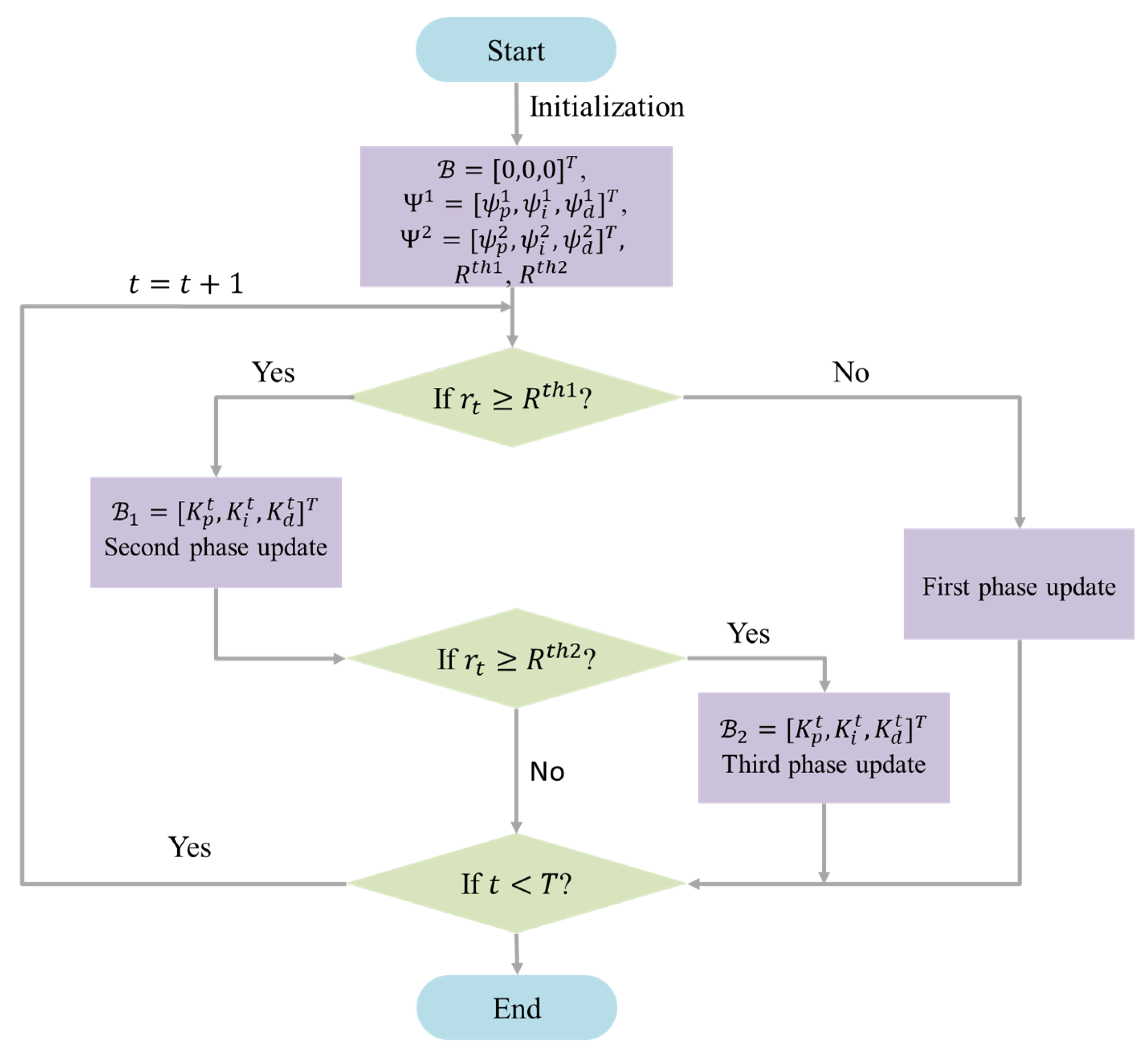
- To balance exploration and exploitation in RL-based PID adaptive tuning, a multi-phase focused PID parameter adaptive tuning framework was proposed based on RL. To ensure the agent’s output PID parameters remain within the stable region, the agent’s action exploration is constrained to remain close to a corresponding reference value of the PID parameters during each phase, a reference value that is then adjusted when the agent performance satisfies a preset reward threshold condition. In this framework, the PID parameter search space is continuously refined from coarse to fine across the training phases, leading to a near-monotonic improvement in the PID parameters’ performance.
- To solve the problem of obtaining a reference value for PID adaptive tuning under the constraint of limited prior knowledge, a mechanism to automatically determine a reference value of the PID parameters was introduced in the multi-phase focusing process. At each phase, the agent automatically establishes a reference value of the PID parameters based on the current phase’s reward threshold and explores within a certain range around this reference value. The reference values established in different phases provide a baseline for the tracking performance of the PID controller, ensuring that the PID controller continuously focuses on improving control performance. The proposed method achieves impressive control performance without prior knowledge of the precise reference values of the PID parameters.
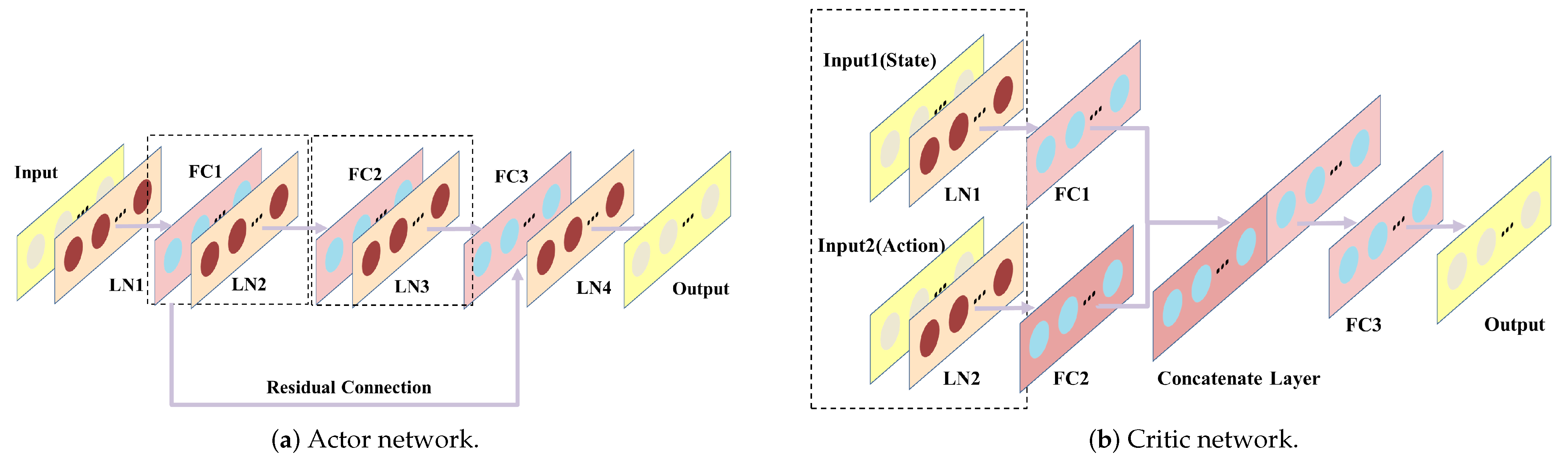
- To address the challenge of a vanishing gradient, which can arise when constraining the output of the actor net of the proposed algorithm, a residual structure was added to the actor net. After applying multi-phase action constraints, the numerical space of the output for the actor net in RL is compressed, leading to a small range of output changes that may cause the gradient to vanish during back-propagation, hindering agent exploration. To overcome this issue, a residual structure was introduced from the shallow layer to the deeper layer of the actor net, preventing the gradient from vanishing and enabling the agent to maintain a certain level of exploration even after multiple action constraints.
1.4. Paper Organization
2. Preliminary Work
2.1. PID Control
2.2. Deep Deterministic Policy Gradient Algorithm
3. Multi-Phase Focused PID Adaptive Tuning with DDPG
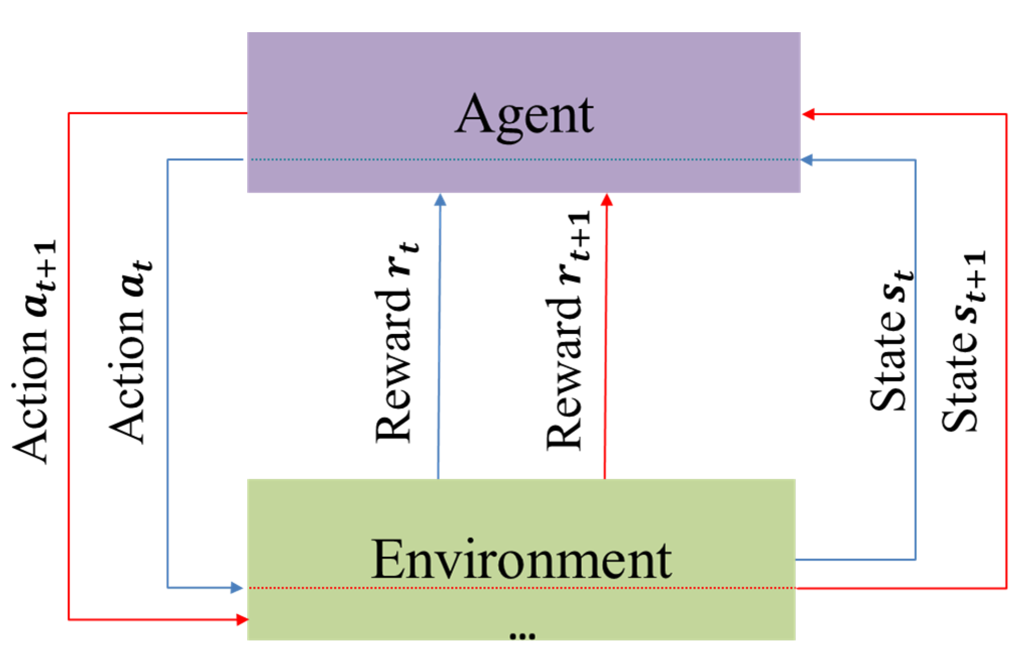
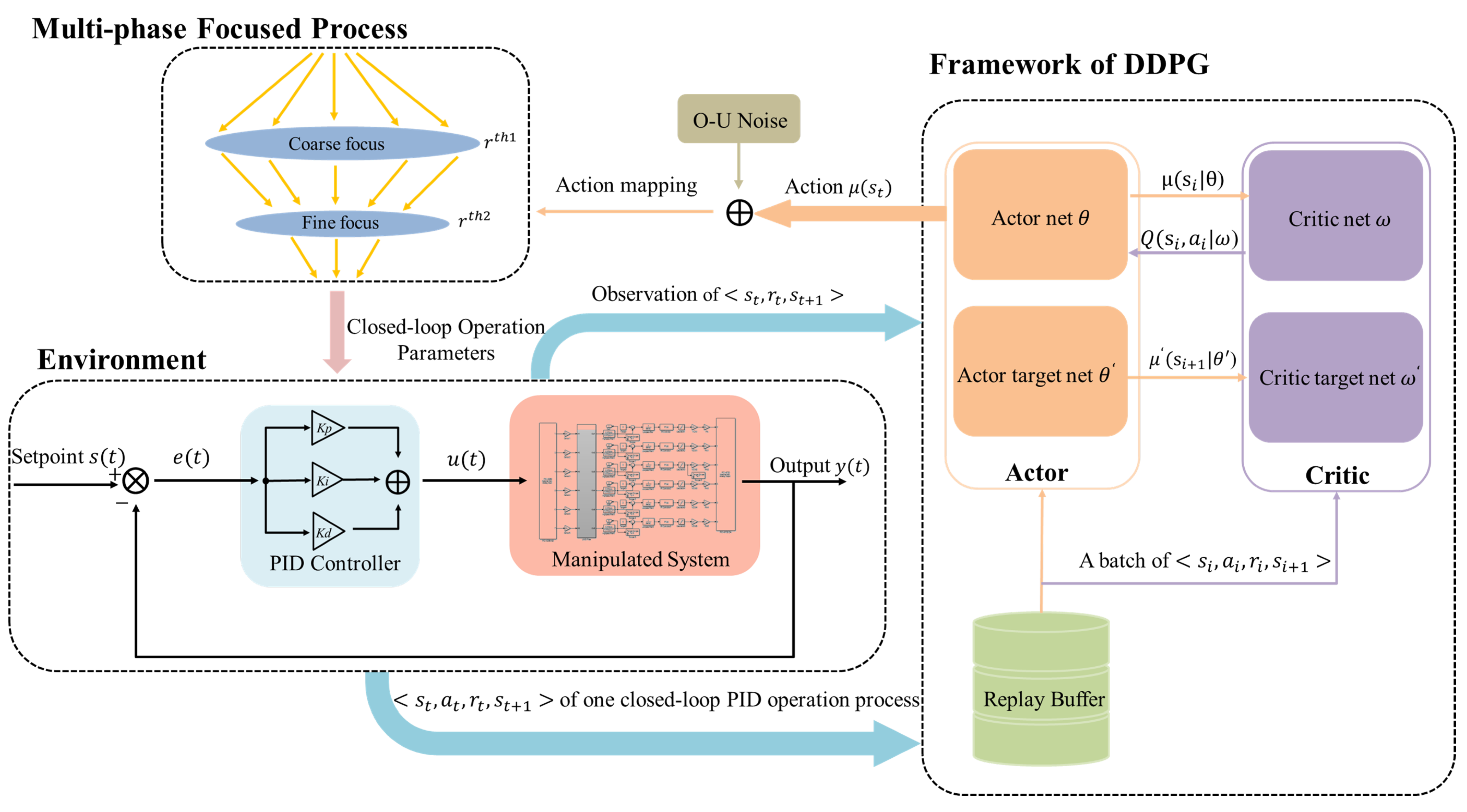
- Environment and agent: The PID closed-loop control operation serves as the environment for the agent, and each step where the PID controller completes a full closed-loop control is an interaction between the agent and the environment. The resulting experience data are stored in the replay buffer. By iteratively learning the agent’s initial random exploration policy, RL aims to eventually learn the environment’s distribution and guide the agent’s exploration towards the optimal policy. To update the critic and actor networks, a set of experience data are randomly selected from the replay buffer every K iterations. The updated actor network then computes the next action based on the current state of the agent, which corresponds to the parameters of the subsequent PID closed-loop operation.
- State and action: The state represents the information obtained by the interaction between the agent and the environment. The agent obtains the reward by evaluating the current state . In the PID control problem, many studies [36,37] take the entire episodic trajectories of inputs and outputs of t-th closed-loop operationandas the state, where L represents the maximum number of time steps of the episodic trajectories. Yet this will introduce the problem of overly high-dimensional inputs to the RL networks. In another study [10], episodic data are described as a state customized to equal the time step, reducing the input dimension, but still potentially resulting in information redundancy. Our observations show that the early stages of the control process exhibit significant output fluctuations, while the output value stabilizes progressively towards the setpoint in the later stages, known as the tuning characteristic of PID control. To capture the impact of the episode’s setting, the time frame with the most pronounced output fluctuations was selected, representing the state of each episode with the first H steps of the closed-loop process. Additionally, in the early stages of exploration, the agent frequently explores the unstable interval of PID parameters, leading to excessive closed-loop operation amplitude and output oscillation, making the output oscillation in the first H steps more noticeable. To address this issue, the system’s output from the previous H steps was normalized and used as the state representation. This simplifies the agent state and reduces network dimension while preserving the observed environmental information. In each episode, the action is the episodic PID parameters , and action is used to guide the episodic PID closed-loop operation.
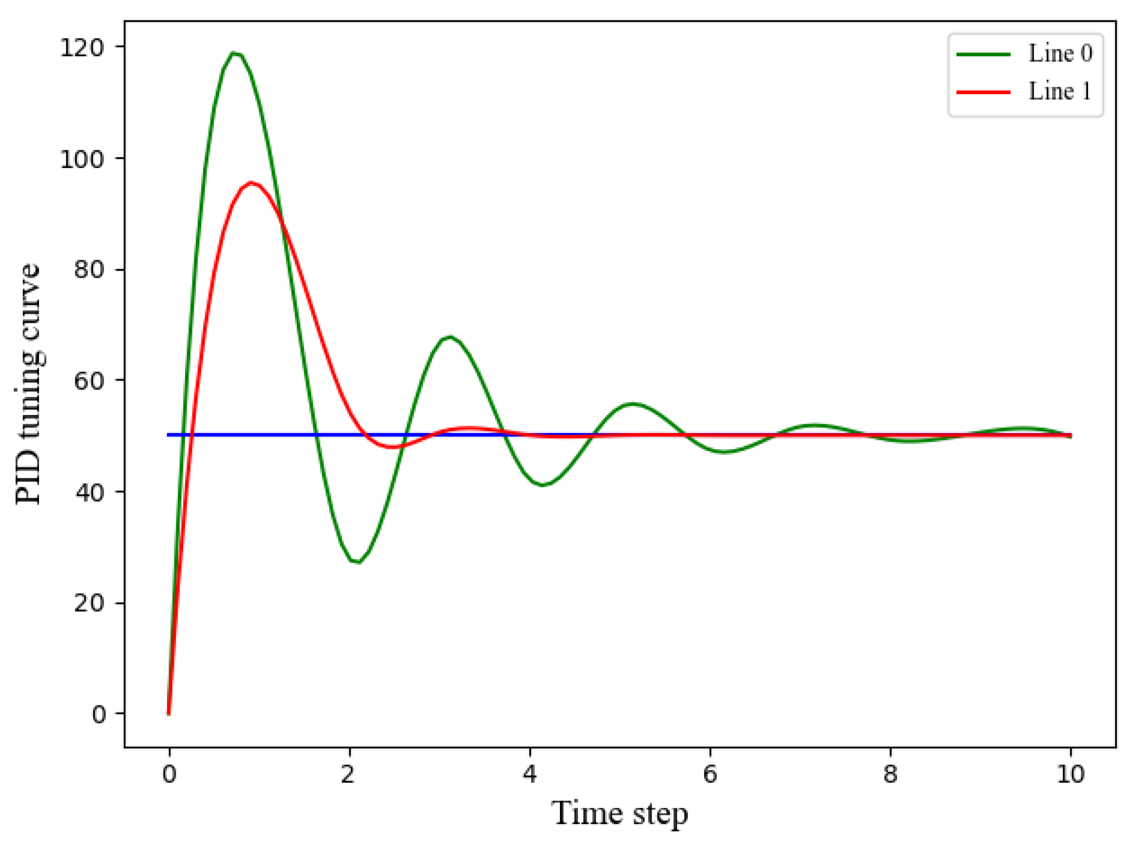
- Reward: To ensure effective control, the reward function of the PID controller should be designed to have a positive correlation with its performance. In particular, the amplitude of the system output should be minimized, as illustrated in Figure 3, and the output should converge to the setpoint rapidly. Accordingly, our reward function incorporates both the time steps and the error of the complete closed-loop trajectories. The reward function is described aswhere , represents the n-th step of the t-th episodic closed-loop operation. The weights of the error and time step in the reward function are denoted by and , respectively. By adjusting these weights, this paper can comprehensively consider trajectory-based metrics of both the error and the number of time steps N during the PID tuning process. This enables us to utilize a trade-off between output amplitude and time steps in reward design. A smaller amplitude of the output corresponds to a shorter time interval and a higher reward. It is worth noting that all rewards are less than 0.
| Algorithm 1 Multi-phase Focused DDPG-based PID Adaptive Tuning Algorithm |
|
4. Experimental Results and Analysis
4.1. Experiment Settings
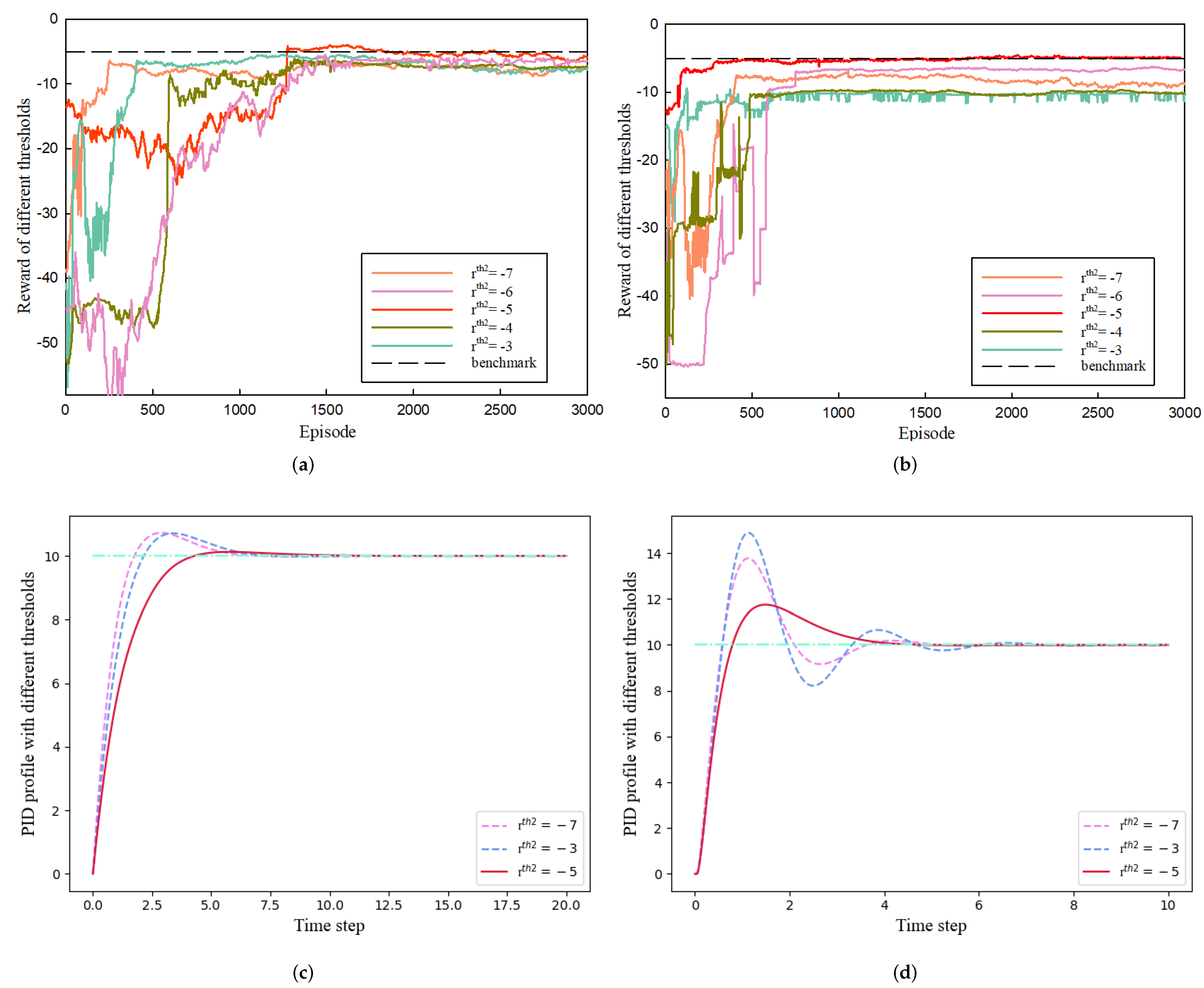
4.2. Threshold Selection Experiment
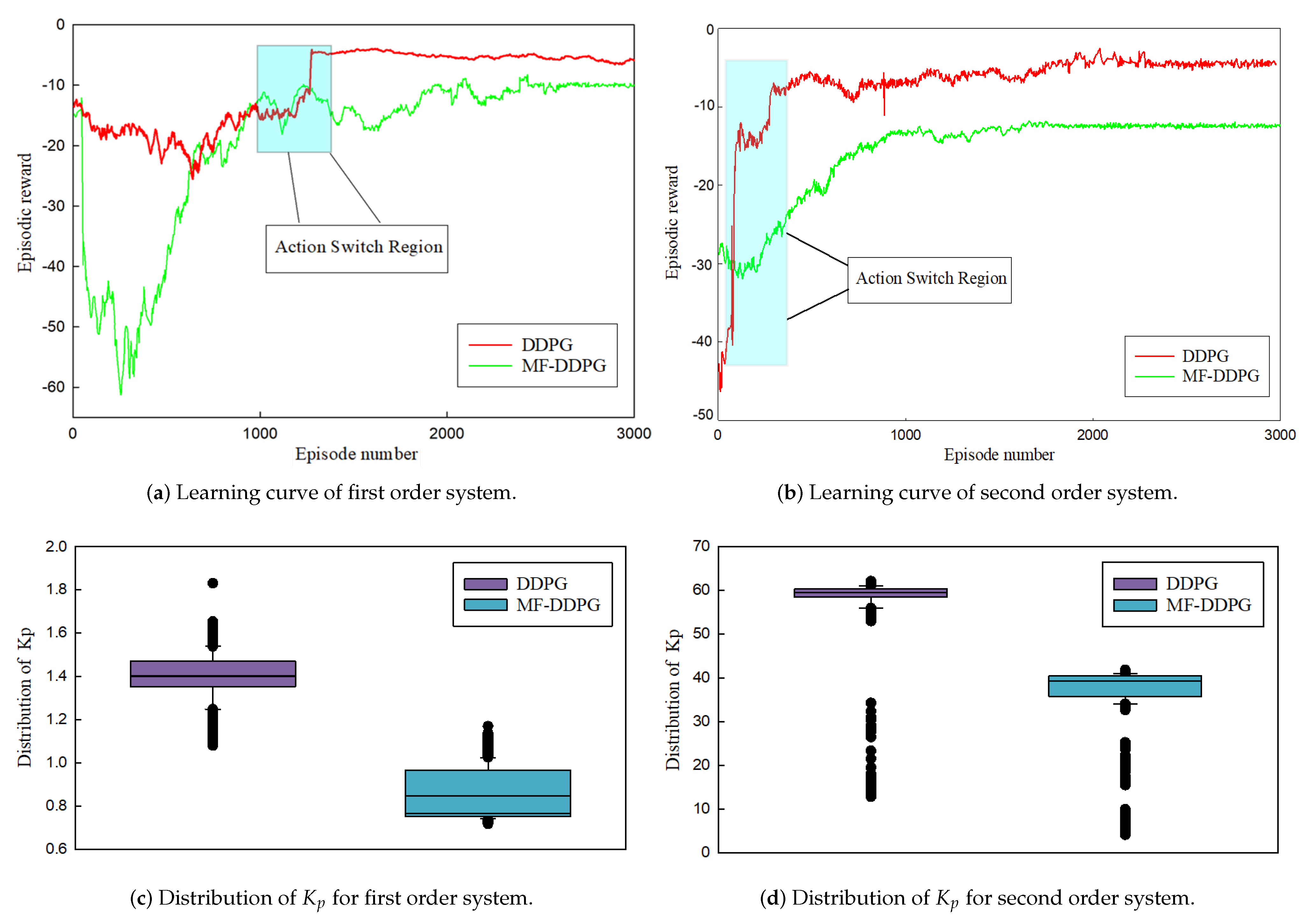
4.3. Experimental Analysis
4.4. Ablation Experiment
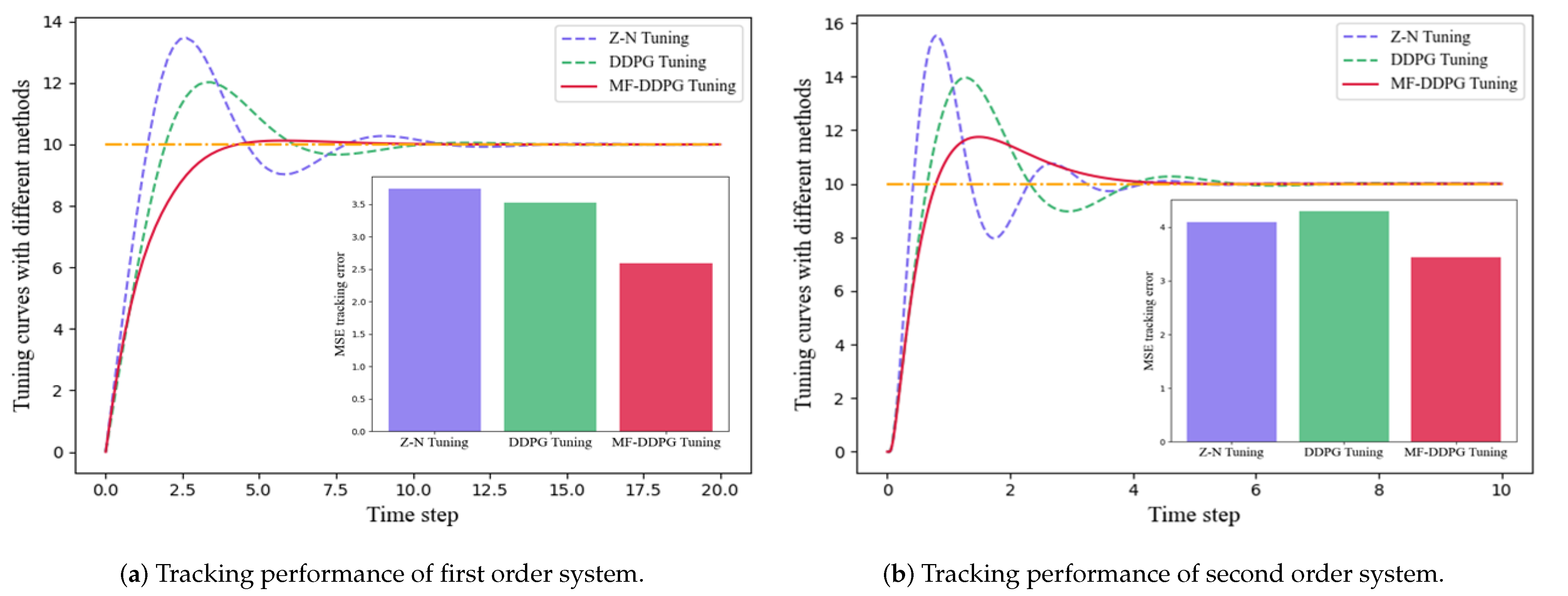
4.5. Comparison with Existing PID Tuning Methods
5. Conclusions
Author Contributions
Funding
Data Availability Statement
Conflicts of Interest
References
- García-Martínez, J.R.; Cruz-Miguel, E.E.; Carrillo-Serrano, R.V.; Mendoza-Mondragón, F.; Toledano-Ayala, M.; Rodríguez-Reséndiz, J. A PID-Type Fuzzy Logic Controller-Based Approach for Motion Control Applications. Sensors 2020, 20, 5323. [Google Scholar] [CrossRef] [PubMed]
- Boubertakh, H.; Tadjine, M.; Glorennec, P.-Y.; Labiod, S. Tuning Fuzzy PD and PI Controllers Using Reinforcement Learning. ISA Trans. 2010, 49, 543–551. [Google Scholar] [CrossRef] [PubMed]
- Borase, R.P.; Maghade, D.K.; Sondkar, S.Y.; Pawar, S.N. A Review of PID Control, Tuning Methods and Applications. Int. J. Dyn. Control 2021, 9, 818–827. [Google Scholar] [CrossRef]
- Yu, D.L.; Chang, T.K.; Yu, D.W. A Stable Self-Learning PID Control for Multivariable Time Varying Systems. Control Eng. Pract. 2007, 15, 1577–1587. [Google Scholar] [CrossRef]
- Lee, D.; Lee, S.J.; Yim, S.C. Reinforcement Learning-Based Adaptive PID Controller for DPS. Ocean Eng. 2020, 216, 108053. [Google Scholar] [CrossRef]
- Wang, L.; Barnes, T.J.D.; Cluett, W.R. New Frequency-Domain Design Method for PID Controllers. IEE Proc.-Control Theory Appl. 1995, 142, 265–271. [Google Scholar] [CrossRef]
- Åström, K.J.; Hägglund, T. The Future of PID Control. Control Eng. Pract. 2001, 9, 1163–1175. [Google Scholar] [CrossRef]
- Bucz, Š.; Kozáková, A. Advanced Methods of PID Controller Tuning for Specified Performance. PID Control Ind. Process. 2018, 73–119. [Google Scholar]
- Bansal, H.O.; Sharma, R.; Shreeraman, P.R. PID Controller Tuning Techniques: A Review. J. Control Eng. Technol. 2012, 2, 168–176. [Google Scholar]
- Lakhani, A.I.; Chowdhury, M.A.; Lu, Q. Stability-Preserving Automatic Tuning of PID Control with Reinforcement Learning. arXiv 2021, arXiv:2112.15187. [Google Scholar]
- Ziegler, J.G.; Nichols, N.B. Optimum Settings for Automatic Controllers. J. Dyn. Syst. Meas. Control 1993, 115, 220–222. [Google Scholar] [CrossRef]
- Cohen, G.H.; Coon, G.A. Theoretical consideration of retarded control. Trans. Am. Soc. Mech. Eng. 1953, 75, 827–834. [Google Scholar] [CrossRef]
- Seborg, D.E.; Edgar, T.F.; Mellichamp, D.A. Process Dynamics and Control; John Wiley & Sons: Hoboken, NJ, USA, 2016. [Google Scholar]
- GirirajKumar, S.M.; Jayaraj, D.; Kishan, A.R. PSO Based Tuning of a PID Controller for a High Performance Drilling Machine. Int. J. Comput. Appl. 2010, 1, 12–18. [Google Scholar] [CrossRef]
- Chiha, I.; Liouane, H.; Liouane, N. A Hybrid Method Based on Multi-Objective Ant Colony Optimization and Differential Evolution to Design PID DC Motor Speed Controller. Int. Rev. Model. Simul. (IREMOS) 2012, 5, 905–912. [Google Scholar]
- Sarkar, B.K.; Mandal, P.; Saha, R.; Mookherjee, S.; Sanyal, D. GA-Optimized Feedforward-PID Tracking Control for a Rugged Electrohydraulic System Design. ISA Trans. 2013, 52, 853–861. [Google Scholar] [CrossRef]
- Lazar, C.; Carari, S.; Vrabie, D.; Kloetzer, M. Neuro-Predictive Control Based Self-Tuning of PID Controllers. In Proceedings of the 12th European Symposium on Artificial Neural Networks, Bruges, Belgium, 28–30 April 2004; p. 395. [Google Scholar]
- Iplikci, S. A Comparative Study on a Novel Model-Based PID Tuning and Control Mechanism for Nonlinear Systems. Int. J. Robust Nonlinear Control 2010, 20, 1483–1501. [Google Scholar] [CrossRef]
- Guan, Z.; Yamamoto, T. Design of a Reinforcement Learning PID Controller. IEEJ Trans. Electr. Electron. Eng. 2021, 16, 1354–1360. [Google Scholar] [CrossRef]
- Kaelbling, L.P.; Littman, M.L.; Moore, A.W. Reinforcement learning: A survey. J. Artif. Intell. Res. 1996, 4, 237–285. [Google Scholar] [CrossRef]
- Sutton, R.S.; Barto, A.G. Reinforcement Learning: An Introduction; MIT Press: Cambridge, MA, USA, 2018. [Google Scholar]
- Astrom, K.J.; Rundqwist, L. Integrator Windup and How to Avoid It. In Proceedings of the 1989 American Control Conference, Pittsburgh, PA, USA, 21–23 June 1989; IEEE: Pittsburgh, PA, USA, 1989; pp. 1693–1698. [Google Scholar]
- Qin, Y.; Zhang, W.; Shi, J.; Liu, J. Improve PID Controller through Reinforcement Learning. In Proceedings of the 2018 IEEE CSAA Guidance, Navigation and Control Conference (CGNCC), Xiamen, China, 10–12 August 2018; IEEE: Xiamen, China, 2018; pp. 1–6. [Google Scholar]
- Zhong, J.; Li, Y. Toward Human-in-the-Loop PID Control Based on CACLA Reinforcement Learning. In Proceedings of the International Conference on Intelligent Robotics and Applications, Shenyang, China, 8–11 August 2019; Springer: Berlin/Heidelberg, Germany, 2019; pp. 605–613. [Google Scholar]
- Carlucho, I.; De Paula, M.; Acosta, G.G. An adaptive deep reinforcement learning approach for MIMO PID control of mobile robots. ISA Trans. 2020, 102, 280–294. [Google Scholar] [CrossRef]
- Carlucho, I.; De Paula, M.; Acosta, G.G. Double Q-PID algorithm for mobile robot control. Expert Syst. Appl. 2019, 137, 292–307. [Google Scholar] [CrossRef]
- Lawrence, N.P.; Stewart, G.E.; Loewen, P.D.; Forbes, M.G.; Backstrom, J.U.; Gopaluni, R.B. Optimal PID and Antiwindup Control Design as a Reinforcement Learning Problem. IFAC-PapersOnLine 2020, 53, 236–241. [Google Scholar] [CrossRef]
- Liu, Y.; Halev, A.; Liu, X. Policy Learning with Constraints in Model-Free Reinforcement Learning: A Survey. In Proceedings of the Thirtieth International Joint Conference on Artificial Intelligence, Montreal, QC, Canada, 19–27 August 2021; International Joint Conferences on Artificial Intelligence Organization: Montreal, QC, Canada, 2021; pp. 4508–4515. [Google Scholar]
- Le, H.; Voloshin, C.; Yue, Y. Batch Policy Learning under Constraints. In Proceedings of the 36th International Conference on Machine Learning PMLR, Long Beach, CA, USA, 10–15 June 2019; pp. 3703–3712. [Google Scholar]
- Bohez, S.; Abdolmaleki, A.; Neunert, M.; Buchli, J.; Heess, N.; Hadsell, R. Value Constrained Model-Free Continuous Control. arXiv 2019, arXiv:1902.04623. [Google Scholar]
- Watkins, C.J.C.H.; Dayan, P. Q-Learning. Mach. Learn. 1992, 8, 279–292. [Google Scholar] [CrossRef]
- Norris, J.R. Markov Chains; Cambridge University Press: Cambridge, UK, 1998. [Google Scholar]
- Silver, D.; Lever, G.; Heess, N.; Degris, T.; Wierstra, D.; Riedmiller, M. Deterministic policy gradient algorithms. In Proceedings of the International Conference on Machine Learning PMLR, Beijing, China, 21–26 June 2014; pp. 387–395. [Google Scholar]
- Sutton, R.S.; McAllester, D.; Singh, S.; Mansour, Y. Policy gradient methods for reinforcement learning with function approximation. Adv. Neural Inf. Process. Syst. 1999, 12, 1057–1063. [Google Scholar]
- Mnih, V.; Kavukcuoglu, K.; Silver, D.; Rusu, A.A.; Veness, J.; Bellemare, M.G.; Graves, A.; Riedmiller, M.; Fidjeland, A.K.; Ostrovski, G.; et al. Human-Level Control through Deep Reinforcement Learning. Nature 2015, 518, 529–533. [Google Scholar] [CrossRef]
- Shin, J.; Badgwell, T.A.; Liu, K.-H.; Lee, J.H. Reinforcement Learning—Overview of Recent Progress and Implications for Process Control. Comput. Chem. Eng. 2019, 127, 282–294. [Google Scholar] [CrossRef]
- Spielberg, S.; Tulsyan, A.; Lawrence, N.P.; Loewen, P.D.; Gopaluni, R.B. Deep Reinforcement Learning for Process Control: A Primer for Beginners. arXiv 2020, arXiv:2004.05490. [Google Scholar]
- Bhatia, A.; Varakantham, P.; Kumar, A. Resource Constrained Deep Reinforcement Learning. Proc. Int. Conf. Autom. Plan. Sched. 2019, 29, 610–620. [Google Scholar] [CrossRef]
- Ioffe, S.; Szegedy, C. Batch Normalization: Accelerating Deep Network Training by Reducing Internal Covariate Shift. In Proceedings of the International Conference on Machine Learning PMLR, Lille, France, 7–9 July 2015; pp. 448–456. [Google Scholar]
- Ba, J.L.; Kiros, J.R.; Hinton, G.E. Layer Normalization. arXiv 2016, arXiv:1607.06450. [Google Scholar]
- Rumelhart, D.E.; Hinton, G.E.; Williams, R.J. Learning Representations by Back-Propagating Errors. Nature 1986, 323, 533–536. [Google Scholar] [CrossRef]
- He, K.; Zhang, X.; Ren, S.; Sun, J. Deep residual learning for image recognition. In Proceedings of the IEEE Conference on Computer Vision and Pattern Recognition, Las Vegas, NV, USA, 27–30 June 2016; pp. 770–778. [Google Scholar]
- Panda, R.C.; Yu, C.-C.; Huang, H.-P. PID Tuning Rules for SOPDT Systems: Review and Some New Results. ISA Trans. 2004, 43, 283–295. [Google Scholar] [CrossRef] [PubMed]


| Parameters | Actor Net | Critic Net |
|---|---|---|
| Structure for networks | [32, 16, 32, 1] | [32, 16, 1] |
| Learning rate | 0.001 | 0.001 |
| Activation function | tanh | relu |
| Replacement factor | 0.01 | 0.01 |
| Optimization function | Adam | Adam |
| Memory size for replay buffer | 2000 | |
| Batch size | 32 | |
| Discount factor | 0.9 | |
| Training length | 3000 | |
| State dimension H | 5 | |
| Parameters | Values (1st) 1 | Values (2nd) 1 |
|---|---|---|
| Reward weights | 10 | 200 |
| Reward weights | 0.1 | 0.001 |
| Reward threshold | −10 | −10 |
| Reward threshold | −5 | −5 |
| Exploration range | [0.15, 0.15, 0.2] | [0.15, 0.15, 0.2] |
| Exploration range | [0.15, 0.15, 0.2] | [0.15, 0.15, 0.2] |
| Episodic length | 20 | 10 |
| Methods | System | |
|---|---|---|
| First-Order System | Second-Order System | |
| MF-DDPG | 2.486 | 3.441 |
| DDPG | 3.483 (28.8%) | 4.295 (19.9%) |
| Z-N | 3.702 (32.8%) | 4.011 (16.0%) |
| Methods | Tracking MSE |
|---|---|
| MF-DDPG | 15.56 |
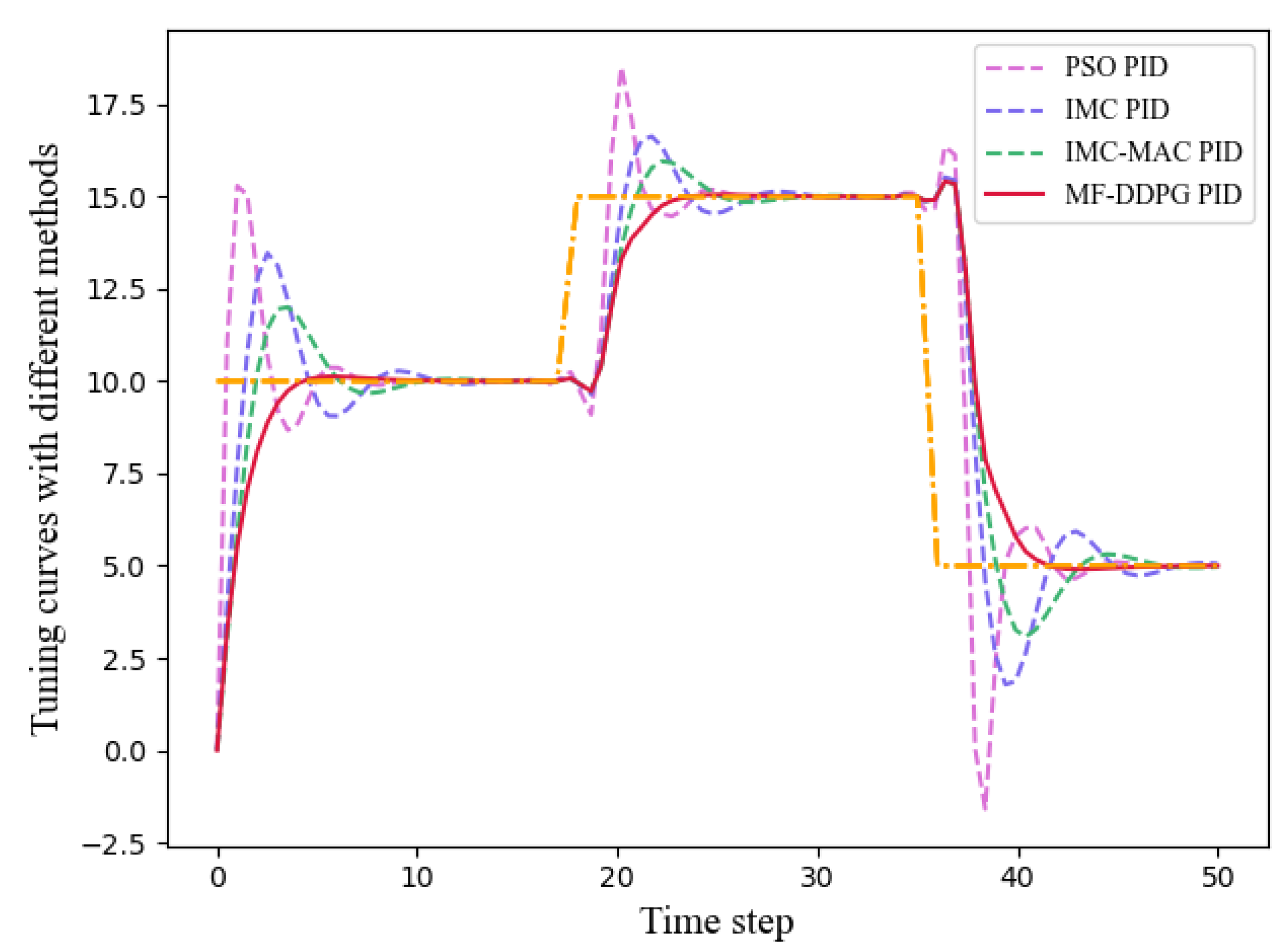
| PSO | 19.63 |
| IMC | 18.52 |
| IMC-MAC | 17.59 |
Disclaimer/Publisher’s Note: The statements, opinions and data contained in all publications are solely those of the individual author(s) and contributor(s) and not of MDPI and/or the editor(s). MDPI and/or the editor(s) disclaim responsibility for any injury to people or property resulting from any ideas, methods, instructions or products referred to in the content. |
© 2023 by the authors. Licensee MDPI, Basel, Switzerland. This article is an open access article distributed under the terms and conditions of the Creative Commons Attribution (CC BY) license (https://creativecommons.org/licenses/by/4.0/).
Share and Cite
Ding, Y.; Ren, X.; Zhang, X.; Liu, X.; Wang, X. Multi-Phase Focused PID Adaptive Tuning with Reinforcement Learning. Electronics 2023, 12, 3925. https://doi.org/10.3390/electronics12183925
Ding Y, Ren X, Zhang X, Liu X, Wang X. Multi-Phase Focused PID Adaptive Tuning with Reinforcement Learning. Electronics. 2023; 12(18):3925. https://doi.org/10.3390/electronics12183925
Chicago/Turabian StyleDing, Ye, Xiaoguang Ren, Xiaochuan Zhang, Xin Liu, and Xu Wang. 2023. "Multi-Phase Focused PID Adaptive Tuning with Reinforcement Learning" Electronics 12, no. 18: 3925. https://doi.org/10.3390/electronics12183925