An Anti-Different Frequency Interference Algorithm for Environment-Aware Millimeter Wave Radar ^†

Abstract

An environment-aware millimeter wave radar (EMWR) is one of the most important sensors in an autonomous driving system. With the increasing penetration of an EMWR on an autonomous vehicle, the possibility of radar interference increases accordingly. Interference may seriously affect the detection performance of an EMWR. When the transmitted signals from other EMWRs are received by the EMWR on an autonomous vehicle, the accuracy of target detection will be affected, which may affect the environment-aware performance. Therefore, more and more attention is paid to how to restrain the interference between EMWR signals. Radar interference can be divided into two types: same-frequency interference (SFI) and different-frequency interference (DFI). In this paper, an anti-DFI algorithm of an EMWR is proposed. Firstly, the causes and signal characteristics of DFI are analyzed. Secondly, the signal amplitude is obtained via Hilbert transform to locate the interference according to the signal characteristics. Then, the Lagrange interpolation based on empirical-mode decomposition (EMD) is used to reconstruct the interference signal to reduce the influence of DFI. Finally, the feasibility of the proposed algorithm is verified by the simulation results. The simulation results validate that the interference signal after EMD filtering and Lagrange interpolation can repair the interference region and achieve the purpose of anti-DFI.

1. Introduction

Nowadays, more and more vehicles have been equipped with advanced driving assistance systems (ADASs), and a large number of ADASs will be equipped with environment-aware millimeter wave radars (EMWRs) in similar frequency bands. Since multiple radars being fired at the same time at the same frequency may cause mutual interference, a vehicle radar needs to achieve effective detection targets in the environment of mutual interference [1,2]. Therefore, research on effective detection with interference and anti-interference methods have received great attention from domestic and foreign manufacturers and standard setting institutions of EMWRs [3,4,5,6]. Radar interference forms can be mainly divided into two types: same-frequency interference (SFI) and different-frequency interference (DFI). The probability of SFI is extremely low, and collisions only occur when two signals are completely identical and the transmission time is exactly the same [7]. For DFI, although the transmission parameters of the radar are inconsistent, some signals fall into the bandwidth received by the radar and are processed as real echo signals [8]. This interference increases the frequency domain noise base and reduces the signal-to-noise ratio (SNR) of the target, which will result in some targets being missed [9,10,11]. If the EMWR does not have the ability to reduce interference effects, it cannot accurately reflect environmental information in real time, and the existence of the radar will be weakened. Based on this issue, the anti-interference ability of EMWRs is increasingly valued. Therefore, the research on EMWRs’ anti-interference technology has important practical significance and application value [12].

The current anti-interference measures for vehicle-mounted millimeter wave radar products at home and abroad can be divided into three categories based on processing location: signal-source-based, signal-transmission-process-based, and received-signal-processing-based [13]. Anti-interference measures based on the signal source are mainly focused on theoretically generating waveforms with good anti-interference characteristics. The anti-interference measures based on the signal transmission process generally rely on phased array radar technology, utilizing its high accuracy, strong anti-interference ability, and high angle resolution characteristics. The anti-interference measures based on received signal processing are achieved by improving the signal processing algorithm aimed at reducing the miss rate and the false alarm rate [14]. Seongwook Lee from the KIM team at Seoul University in South Korea proposed using wavelet transform to extract interference signals from low-pass filtered output signals, thereby suppressing interference [3]. However, the selection of an appropriate wavelet basis function is a challenge. An improved weighted envelope normalization method was proposed to reduce the interference amplitude and thereby improve the SNR of the real targets detected by an EMWR. After suppression, the normal signal of the radar is damaged, and if it takes a long time, it will have an impact on the subsequent tracking of the radar, which still causes the missing detection of the target [15]. In 2021, Jiang Liubing’s team from Guilin University of Electronic Science and Technology proposed an anti-interference method that combines empirical-mode decomposition (EMD) and autoregressive model [16]. The main idea is to decompose the interference modes in the echo signal through mode decomposition and then use adaptive regression to reconstruct the suppressed echo signal. The simulation results show that this method can effectively suppress high-frequency interference, but the reconstruction time and parameters of empirical-mode decomposition are difficult to maintain consistency in different signals [17].

In this paper, a Hilbert transform for interference location method and a Lagrange interference mitigation method after EMD filtering are proposed based on the analysis of the characteristics of DFI. Then, the feasibility of the scheme is verified via simulation, and the proposed method can achieve an ideal effect. This method can also fit well in anti-DFI, and the amount of calculation is not complicated, which is conducive to practical application. The rest of this paper is organized as follows: Section 2 analyzes the characteristics of radar signals and DFI signals. Section 3 describes the proposed Hilbert method for interference location and the Lagrange interpolation algorithm based on EMD. Section 4 presents the implementation steps of the anti-DFI algorithm and analyzes the simulation results to verify the feasibility of the proposed anti-DFI algorithm. Finally, this paper is concluded in Section 5.

2. Analysis of DFI

This section analyzes the characteristics of DFI from the aspects of a radar system and radar processing flow and deduces the echo model of DFI and the influence of interference signals on radar detection results.

2.1. Radar Signal Analysis

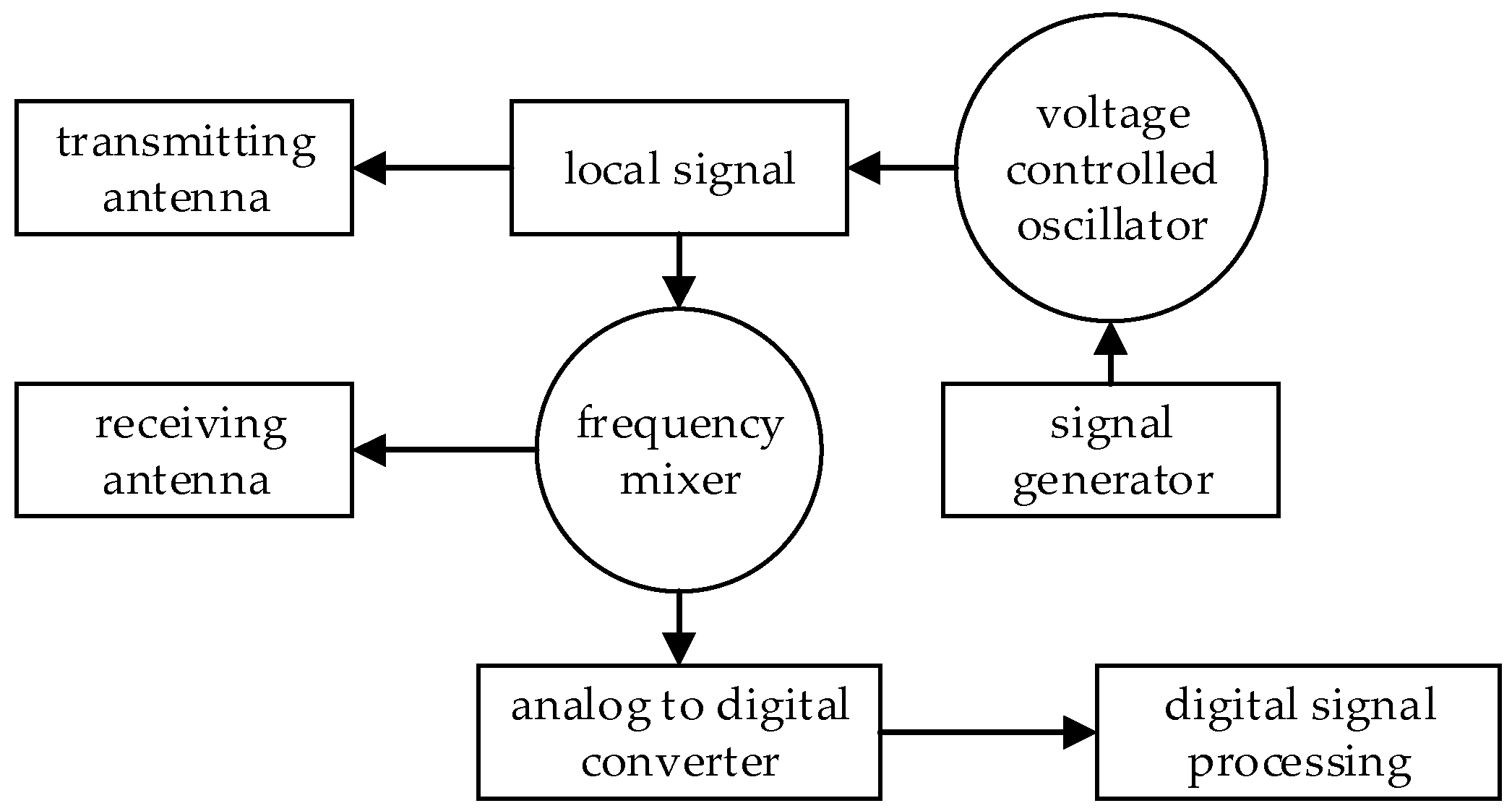
At present, EMWRs mostly use the principle of linear frequency modulated continuous wave (LFMCW) to realize radar ranging and velocity measurement [17]. The working block diagram of the system is shown in Figure 1:

The transmitting antenna of the radar is tasked with transmitting high-power RF signals, which are transmitted to the antenna through the feeder for radiation. The task of the radar-receiving antenna is to receive the reflected electromagnetic wave signal. The target echo signal and interference signal received by the radar are amplified by the high-frequency amplifier with a low noise and then transmit to the mixer. The high-frequency signal in the local oscillator and the received signal are mixed in the mixer for data acquisition and sent to the data processing unit for processing.

The expression of the signal transmitted by the EMWR is

$$\begin{array}{l}m(t)=M_t\cos (2\pi ft+\pi k{t}^2)\\ k=\frac{B}{T_p}\end{array},$$

(1)

where $M_t$ is the transmitting gain; $f$ is the start frequency of the signal; $k$ is the sweep slope; $B$ is the bandwidth of the signal; $T_p$ is the pulse width of the signal.

The echo signal after the reflection by the target is

$$r(t)=M_t{M}_r\cos (2\pi (f+f_d)(t-\tau )+\pi k{(t-\tau )}^2),$$

(2)

where $M_r$ is all gains in the receiving process, including the receiving antenna gain, target RCS, and spatial attenuation; $f_d$ is the Doppler information introduced by target motion; $\tau$ is the delay time, which is related to the distance of the target [18,19]. The signal after mixing with the mixer is

$$s(t)=M_t{M}_r\cos (-2\pi f\tau -2\pi kt\tau +\pi k{\tau }^2+2\pi f_d(t-\tau )),$$

(3)

The signal collected via the ADC with the sampling rate $f_s$ is

$$S(n)=M_t{M}_r\cos (-2\pi f\tau -\frac{2\pi kn\tau }{f_s}+\pi k{\tau }^2+2\pi f_d(\frac{n}{f_s}-\tau )),$$

(4)

When the target is stationary, $f_d$ is equal to 0, and the signal in Equation (4) is reducible to

$$S(n)=M_t{M}_r\cos (-2\pi f\tau -\frac{2\pi Bn\tau }{N}+\pi \frac{B{f}_s}{N}{\tau }^2),$$

(5)

The signal transformed by DFT is

$$S(w)={\displaystyle \sum _{n=0}^{N-1}S(n)e^{-j\frac{2\pi }{N}wn}},$$

(6)

It can be found from Equation (6) that $S(w)$ will have a peak value in $B\tau$. That is to say, the Fourier transform of the received signal will produce a peak in the position corresponding to the distance of the target, and the rest of the position is noise. The principle of velocity measurement is the same as the above distance analysis. In conclusion, the detection ability of the FMCW signal can be proved.

2.2. Radar Signal with DFI Analysis

When the radar is interfered, the received signal includes the echo signal and interference signal. The relationships between the interference signal, local oscillator signal. and echo signal are shown in Figure 2.

According to the above process, the echo signal is

$$r(t)=M_t{M}_r\cos (2\pi f(t-\tau )+\pi k{(t-\tau )}^2)+M_i\cos (2\pi f_{i}t+\pi k_i{t}^2),$$

(7)

where $M_i$ is the gain of the interference signal; $f_i$ is the initial frequency of the interference signal; $k_i$ is the slope of the interference signal. Affected by the IF filter of the radar, the interference signal after mixing with the mixer is

$$\begin{array}{ll}s(t)=& M_t{M}_r\cos (-2\pi f\tau -2\pi kt\tau +\pi k{\tau }^2)\\ & +rectpuls(t-t_1,\Delta t)M_i\cos (2\pi (f_i-f)t+\pi \left(k_i-k\right)t^2)\end{array},$$

(8)

The signal after ADC collection is

$$\begin{array}{ll}S(n)& =M_t{M}_r\cos (-2\pi f\tau -\frac{2\pi Bn\tau }{N}+\pi \frac{B{f}_s}{N}{\tau }^2)\\ & +rectpuls(n-n_1,\frac{\Delta t}{f_s})M_i\cos (2\pi (f_i-f)\frac{n}{f_s}+\pi \left(k_i-k\right){(\frac{n}{f_s})}^2),\end{array}$$

(9)

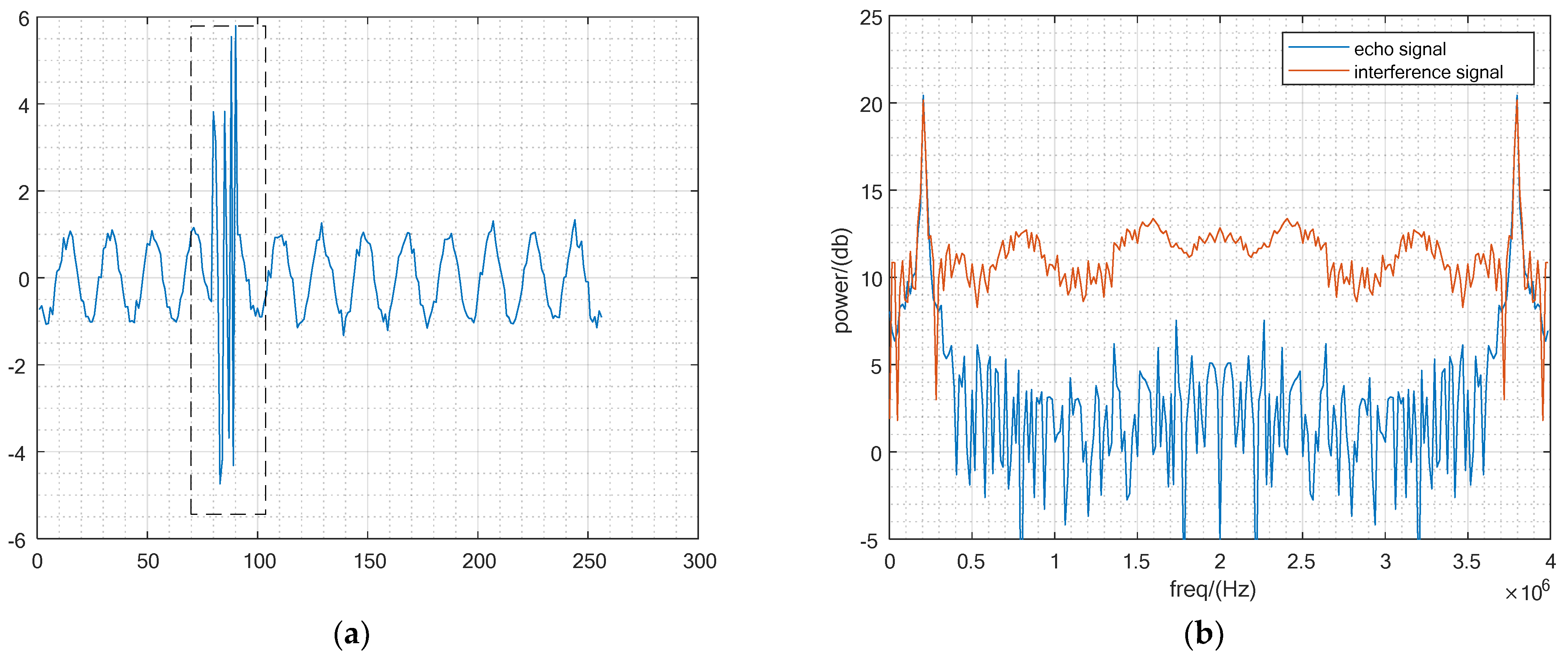
where $rectpuls$ is the rectangular wave, and the starting time is $t_1$ with the pulse of $\Delta t$. The signal consists of two parts. One is a signal with a fixed frequency introduced by the target, and the other is a signal with bandwidth $f_N$ introduced by interference. For the radar signal, $f_N$ is equal to $f_s/2$. Therefore, when there is an interference in the radar system, the energy in the entire band will be increased, which is shown in Figure 3.

Figure 3a is the ADC of the DFI signal. In Figure 3b, the blue line is the FFT results for the echo signal, and the red line is the FFT results for the interference signal. It can be seen from Figure 3b that the bottom noise will be raised on all distance gates after Fourier transform. Therefore, if the noise power is higher than the target power, it will cause these targets to be undetected, which is called a missing alarm. The detection range of the radar needs to be reduced to meet the same SNR before interference, so the range will be shorter than before.

3. Anti-DFI Algorithm

Through the analysis of the interference characteristics in the previous section, this section provides a detailed explanation and simulation of the anti-DFI algorithm by recovering the interference signal after determining the interference position.

Before introducing the anti-interference algorithm in this article, we first introduce a time-domain anti-interference technology based on time shift. The core idea of time-domain anti-interference technology is to reduce the time-domain overlap between the test radar and the interference radar transmission signal.

Assuming that the time interval between the test radar and the interference radar signal is $t_a$, and the maximum interference frequency of the low-pass filter processing IF signal that is not affected is $f_a$, the relationship between the two radar signals is

$$t_a=\frac{f_a}{k},$$

(10)

where k is the Ramp slope. The probability of interference occurring can be expressed as

$$P(interference)=\frac{2t_a{N}_{chirp}}{T},$$

(11)

where $N_{chirp}$ is the number of chirp signals continuously transmitted, and T is the fixed transmission period and is usually set to 50 ms.

According to the formula, by changing the fixed transmission period of the radar, the probability of interference can be reduced. The simplest way is to increase the idle time $T_I$ between chirps. The setting value of $T_I$ needs to consider both the Ramp bandwidth and the descent stability time. Therefore, the reference value for setting the step time $\Delta t$ of $T_I$ is

$$\Delta t=\frac{T(T_m-2t_a)}{2t_a{N}_{chirp}},$$

(12)

From the above analysis, it can be concluded that the time-domain anti-interference method based on time shift has a good suppression effect on parallel interference between radars using the same chirp parameters and the same frame configuration, as it separates the signal between the test radar and the jamming radar within the receiving bandwidth from a time-domain perspective. However, the theoretical suppression effect is limited for interference that already overlaps between the test radar and the jamming radar. For this purpose, this article conducts corresponding suppression processing on the signal in the frequency domain, and the specific process is given as follows.

3.1. Hilbert Transformation

For any signal $f(t)$, its Hilbert transformation form is recorded as $h(t)=H[f(t)]$, defined as

$$\left\{\begin{array}{l}h(t)=\frac{1}{\pi }{\displaystyle \int \frac{f\left(\tau \right)}{t-\tau }d\tau }\\ f(t)=\frac{-1}{\pi }{\displaystyle \int \frac{h\left(\tau \right)}{t-\tau }d\tau },\end{array}\right.$$

(13)

Thus, the Hilbert transformation of any signal $f(t)$ is equivalent to the convolutional calculation with $1/\pi t$. The impact response and frequency response of the Hilbert converter are shown as

$$\left\{\begin{array}{l}x(t)=\frac{1}{\pi t}\\ X(jw)={\displaystyle \int \frac{1}{\pi t}{e}^{-jwt}dt=-j\ast sign(w),}\end{array}\right.$$

(14)

where $sign(w)$ is a symbol function. In summary, the essence of Hilbert transformation is a $2/\pi$ phase of the frequency of the input signal. The signal after Hilbert transformation is

$$\begin{array}{l}\widehat{S}(n)=M_t{M}_r\sin ({\widehat{t}}_1)+rectpuls(n-n_1,\frac{\Delta t}{f_s})M_i\sin ({\widehat{t}}_2)\\ {\widehat{t}}_1=-2\pi f\tau -\frac{2\pi Bn\tau }{N}+\pi \frac{B{f}_s}{N}{\tau }^2\\ {\widehat{t}}_2=2\pi (f_i-f)\frac{n}{f_s}+\pi \left(k_i-k\right){(\frac{n}{f_s})}^2,\end{array}$$

(15)

The envelope of the signal is

$$\sqrt{S^2+{\widehat{S}}^2}=\left\{\begin{array}{l}{M}_t{M}_r\begin{array}{cc}& no\begin{array}{c}\end{array}interference\end{array}\\ \sqrt{M_t{}^2{M}_r{}^2+M_i^2+2M_t{M}_r{M}_i\cos ({\widehat{t}}_1-{\widehat{t}}_2)}\begin{array}{cc}& interference\end{array}\end{array}\right.,$$

(16)

In summary, the signal contour can be obtained via Hilbert transformation to locate the interference position. After acquiring the envelope through Hilbert transformation, we need to delimit a reasonable threshold. It can be seen from the envelope that when the radar is disturbed by a different frequency, the signal amplitude will rise greatly. Therefore, the threshold can be reasonably delimited according to the relationship between the median and the maximum value of the envelope. The formula for delimiting the threshold is median + (maximum-median) × n%, where n is the correlation proportional coefficient.

3.2. Interpolation Algorithm

After the Hilbert transformation, the position of the interference is reconstructed. The Lagrange interpolation algorithm is used for the signal reconstruction in this subsection.

A known function $y=f\left(x\right)$ in $n+1$ points $[x_0,x_1\dots x_n]$ is corresponding with $[y_0,y_1\dots y_n]$, where $[x_0,x_1\dots x_n]$ are different with each other. An n-order polynomial can be constructed as $y=P_n\left(x\right)$, $P_n\left(x_k\right)=y_k,k=0,1\dots n$. We define the interpolation polynomial as

$$P_n(x)={\displaystyle \sum _{k=0}^n{y}_k{p}_k(x)},$$

(17)

So, the formula needs to satisfy

$$p_k\left(x_j\right)=\left\{\begin{array}{c}1, j=k\\ 0,j\ne k\end{array}\right.,$$

(18)

where $j=0,1,\cdots , n$ and $k=0,1,\cdots , n$. The n-order polynomial in Equation (14) is called an interpolation base function. The Lagrange basic polynomial is defined as

$$p_k(x)=\frac{(x-x_0)\dots (x-x_{k-1})(x-x_{k+1})\dots (x-x_n)}{(x_k-x_0)\dots (x_k-x_{k-1})(x_k-x_{k+1})\dots (x_k-x_n)},$$

(19)

Five interference points are assumed in the signal. The Lagrangian interpolation coefficient of the base 10 interpolation of each five points before and after is used. Coefficients are shown in

Table 1. Lagrange interpolation coefficients.

$\mathit{n}$	${\mathit{P}}_0$	${\mathit{P}}_1$	${\mathit{P}}_2$	${\mathit{P}}_3$	${\mathit{P}}_4$	${\mathit{P}}_5$	${\mathit{P}}_6$	${\mathit{P}}_7$	${\mathit{P}}_8$	${\mathit{P}}_9$
1	0.0839	−0.6294	1.9580	−3.1818	2.7273	0.4545	−0.9091	0.7343	−0.2797	0.0420
2	0.2098	−1.5105	4.4056	−6.3636	4.0909	1.6364	−3.1818	2.5175	−0.9441	0.1399
3	0.2797	−1.9580	5.4825	−7.4242	4.2424	3.1818	−5.9394	4.5688	−1.6783	0.2448
4	0.2448	−1.6783	4.5688	−5.9394	3.1818	4.2424	−7.4242	5.4825	−1.9580	0.2797
5	0.1399	−0.9441	2.5175	−3.1818	1.6364	4.0909	−6.3636	4.4056	−1.5105	0.2098

.

During the calculation of Lagrange interpolation, the introduced noise of the ADC signal causes noise amplification through the $p_k(x)$ coefficient during the interpolation process. The amplification noise is

$$noise={\displaystyle \sum _{k=0}^n{p}_{k}randn(k)},$$

(20)

Due to the amplification of the noise, the error in the interpolation process becomes larger, and the results are shown in Figure 4.

As shown in Figure 4, the error introduced by the Lagrange coefficient cannot be ignored due to the existence of noise. In the process of signal reconstruction, the noise energy of some range gates decreases, while the noise of some range gates increases, which is not conducive to target detection. Therefore, the empirical-mode decomposition (EMD) method is used to simply filter the signal.

Before performing EMD, time–frequency processing [20] is performed on the signal and a sliding window is added to the analyzed signal. Assuming that the signal within the short-term window is stationary, the window function is moved and then the Fourier transform of the signal within each short-term window is calculated to obtain the time–frequency distribution of the signal, which is defined as

$$S\left(t,f\right)={\displaystyle \underset{\infty }{\int }s\left(\tau \right)g\left(\tau -t\right)e^{-j2\pi f\tau }d\tau },$$

(21)

where $g(t)$ is the window function, and $s(t)$ is the signal to be analyzed.

The EMD algorithm is a method of signal decomposition to obtain characteristic modes proposed by NE. Huang et al. [21]. The advantage of the EMD algorithm is that it can be used to adaptively generate intrinsic mode functions based on the analyzed signal instead of using any already-defined function as the substrate. It can be used to analyze nonlinear, non-stationary signal sequences, with a very high SNR and good time–frequency focus. The basic principle of the EMD algorithm is:

(1)

The maximum and minimum points of the original signal are found and then fitted via curve interpolation to obtain the upper and lower envelope of the signal.

(2)

The upper and lower envelopes are averaged to obtain the average envelope.

(3)

The original signal minus the mean envelope signal is used to obtain the residual signal. The above is repeated for the remaining signals until the screening threshold is less than a certain threshold to obtain the final appropriate first-order mode component.

(4)

The original signal and the first-order mode component are subtracted to obtain the first-order residue quantity. After replacing the original signal, the above processing step is repeated n times to obtain the n-order mode function and the final residual amount that meets the standard.

In this paper, the cross-correlation analysis of the decomposed intrinsic mode function (IMF) of EMD with the original noise-free simulated signal is carried out. When the threshold value is less than a certain value, it is considered as noise. The IMF results after two decompositions are shown in Figure 5.

The cross-correlation results are shown in

Table 2. The cross-correlation result.

IMF	IMF1	IMF2	Interference Signal
cross-correlation	0.1219	0.9678	0.6411

. It can be seen that the cross-correlation between IMF2 and the original non-noise signal is high, which means the similarity between the two signals is high, while the signal similarity of IMF1 is poor. And the correlation of the IMF2 signal is higher than the original interference signal, so the first-order modal component of EMD can be considered as the noise signal, and IMF2 is the filtered signal.

4. Simulation Results and Analysis

In this section, the simulation parameters are set as carrier frequency = 77 GHz, sampling frequency = 10 MHz, and bandwidth = 50 MHz. Hilbert transform, the EMD filter, and the Lagrange interpolation algorithm are used to process the interfered radar signal and to reduce the influence of DFI on radar detection. The specific steps are as follows:

Step 1: Obtain the signal envelope based on Hilbert transformation;

Step 2: Reasonably delimit the threshold and intercept the interference range of the interference signal;

Step 3: Decompose the undisturbed signal via EMD to isolate the effective signal;

Step 4: Relying on the effective signal, build the Lagrange basic polynomial, and interpolate the interference part to alleviate the interference.

The original signal and Hilbert transformation envelope signal are shown in Figure 6.

As shown in Figure 6, the red line is the interference signal, the blue line is the envelope of the signal after the Hilbert transform, and the yellow line is the delimited threshold. The Hilbert transform can acquire the profile of the signal, and the delimited threshold can delimit the corresponding threshold to intercept the interference range according to the contour, so as to determine the position of the interference signal. After locating to the interference position, the Lagrange polynomial is constructed through the undisturbed data, and the interference part is interpolated. In this section, five points are selected before and after the interference time period. According to the principle of Lagrange interpolation, the interference signal with EMD filtering and the signal without EMD filtering are interpolated. The results are shown in Figure 7.

As shown in Figure 7, the red line is the interpolated signal with EMD filtering, and the blue line is the interpolated signal without EMD filtering. It can be seen that the Lagrange interpolation signal without EMD filtering is unsatisfactory due to the influence of noise and the relatively poor peak side lobe ratio (PSLR) of the signal after Fourier transform. So, when there are other weak targets near the target, the interpolated signal without EMD filtering, the radar will not detect it and cause a false alarm of the radar. In addition, due to the lifting of the bottom noise around the target, the radar may detect the false target, resulting in radar omission. After EMD filtering, the situation will be greatly alleviated, and the PSLR at the target is about 15dB, and the detection of the weak target will be unaffected.

In conclusion, the amplitude information is obtained via Hilbert transform, and then, the interference location is carried out. Then, the interference signal after EMD filtering is interpolated via the Lagrange interpolation method to restore the original ADC signal, which can repair the interference region and achieve the purpose of anti-DFI.

5. Conclusions

This paper mainly studies the working principle, interference characteristics, and anti-DFI algorithm of EMWRs. Based on the characteristics and interference mechanism of DFI, an envelope extraction method based on Hilbert transform is proposed to determine the interference location. Then, the non-interference signal is filtered via the EMD algorithm, and the interference part is interpolated via the Lagrange interpolation algorithm to remove the influence of DFI. Finally, the practicability of this method is verified via theoretical simulation. The simulation results validate that the interference signal after EMD filtering and Lagrange interpolation can repair the interference region and achieve the purpose of anti-DFI.

Although the anti-DFI algorithm has been theoretically simulated in this paper, the interference scenario set in this experiment is a little monotonous. And more experiments on anti-interference technology in more complex interference scenarios are needed in the future to conduct in-depth research in this direction.

References

- Hasch, J.; Topak, E.; Schnabel, R.; Zwick, T.; Weigel, R.; Waldschmidt, C. Millimeter-wave technology for automotive radar sensors in the 77 GHz frequency band. IEEE Trans. Microw. Theory Tech. 2012, 60, 845–860. [Google Scholar] [CrossRef]
- Nozawa, T. An anti-collision automotive FMCW radar using time domain interference detection and suppression. In Proceedings of the International Conference on Radar Systems (Radar 2017), Belfast, Ireland, 23–26 October 2017; pp. 1–5. [Google Scholar]
- Lim, S.; Lee, S.; Choi, J.-H.; Yoon, J.; Kim, S.-C. Mutual interference suppression and signal restoration in automotive FMCW radar systems. IEICE Trans. Commun. 2018, 10, 10–15. [Google Scholar] [CrossRef]
- Liu, H.; Duan, F.; Li, J.; Li, F.; Zhong, G. Preprocessing method of blade tip timing signal based on spatial transformation. Chin. J. Sci. Instrum. 2022, 43, 218–229. [Google Scholar]
- Hu, T.; Shao, X.; Xiao, M.; Li, F.; Xue, W.; Xiao, Z. Methods of anti-radar emitter signal jamming for linear frequency modulated continuous wave detector. Chin. J. Sci. Instrum. 2022, 43, 253–260. [Google Scholar]
- Huan, H.; Tao, R.; Li, Y.; Wang, Y.; Wang, G. Co-channel interference suppression for homo-type radars based on joint transform domain and time domain. J. Electron. Inf. Technol. 2012, 34, 2978–2984. [Google Scholar] [CrossRef]
- Li, F.; Xu, J.; Zhang, X. Pulse jamming suppression for airborne radar based on joint time-frequency analysis. In Proceedings of the IET International Radar Conference, Xi’an, China, 14–16 April 2013; pp. 1–4. [Google Scholar]
- Zhang, H.; Wang, R.; Wan, J. LFMCW radar ranging method with high precision based on IRife algorithm. J. Electr. Meas. Instrum. 2017, 31, 251–256. [Google Scholar]
- Ren, M.; Yan, G.; Zhu, Y.; Wang, Z.; Gao, T. Study on radar anti-jamming performance test method in complex electromagnetic environment. Chin. J. Sci. Instrum. 2016, 37, 1277–1282. [Google Scholar]
- Elgmel, S.; Soraghan, J. Using EMD-FrFT filtering to mitigate very high power interference in chirp tracking radars. IEEE Signal Process. Lett. 2011, 18, 263–266. [Google Scholar] [CrossRef]
- Zhao, Z.; Shi, X. FM interference suppression for PRC-CW radar based on adaptive STFT and time-varying filtering. J. Syst. Eng. Electron. 2010, 21, 219–223. [Google Scholar] [CrossRef]
- Chen, L.; Chen, D.; Liu, Y. A new chirp signal parameter estimation algorithm. Acta Armamentarii 2014, 35, 207–213. [Google Scholar]
- Chen, S.; Taghia, J.; Kuhnau, U.; Martin, R. Automotive radar interference mitigation based on a generative adversarial network. In Proceedings of the IEEE Asia-Pacific Microwave Conference (APMC), Hong Kong, 8–11 December 2020; pp. 728–730. [Google Scholar]
- Mun, J.; Ha, S.; Lee, J. Automotive radar signal interference mitigation using RNN with self attention. In Proceedings of the IEEE International Conference on Acoutics, Speed and Signal Processing, Barcelona, Spain, 4–8 May 2020; pp. 3802–3806. [Google Scholar]
- Ma, L.; Zhao, Y. Signal processing for automobile anti-collision radar. Electron. Technol. Softw. Eng. 2018, 20, 82–83. [Google Scholar]
- Tang, B.; Zhao, Y.; Cai, T. Advances and perspective in radar ECCM techniques of active jamming. J. Data Acqusition Process. 2016, 31, 623–639. [Google Scholar]
- Fan, Y.; Pan, Z.S.; Wang, Z. Wavelet Theory Algorithm and Filter Group; Science Press: Beijing, China, 2011; pp. 60–61. [Google Scholar]
- Xu, T.; Yu, D.; Du, L. A Bi-Objective Simulation Facility for Speed and Range Calibration of 24 GHz and 77 GHz Automotive Millimeter-Wave Radars for Environmental Perception. Electronics 2023, 12, 2947. [Google Scholar] [CrossRef]
- Du, L.; Sun, Q.; Bai, J.; Wang, J. A Verification Method for Traffic Radar-Based Speed Meter with Target Position Determination in Road Vehicle Speeding Enforcement. IEEE Trans. Veh. Technol. 2021, 70, 12374–12388. [Google Scholar] [CrossRef]
- Elouaham, S.; Latif, R.; Dliou, A.; Maoulainine, F.; Laaboubi, M. Biomedical signals analysis using time-frequency. In Proceedings of the 2012 IEEE International Conference on Complex Systems (ICCS), Agadir, Morocco, 5–6 November 2012; pp. 1–6. [Google Scholar]
- Hartley, J.D. A method for suppression of pulsed interference in a pulse Doppler radar. In Proceedings of the IEEE International Conference on Radar, Adelaide, SA, Australia, 2–5 September 2008; pp. 265–270. [Google Scholar]