

Multimodal Global Trajectory Planner for Autonomous Underwater Vehicles


Faculty of Mechanical and Electrical Engineering, Polish Naval Academy, 81-127 Gdynia, Poland
Electronics 2023, 12(22), 4602; https://doi.org/10.3390/electronics12224602
Submission received: 29 September 2023
/
Revised: 27 October 2023
/
Accepted: 7 November 2023
/
Published: 10 November 2023
(This article belongs to the Special Issue Feature Papers in Electrical and Autonomous Vehicles)
Abstract
:The underwater environment introduces many limitations that must be faced when designing an autonomous underwater vehicle (AUV). One of the most important issues is developing an effective vehicle movement control and mission planning system. This article presents a global trajectory planning system based on a multimodal approach. The trajectory of the vehicle’s movement has been divided into segments between introduced waypoints and calculated in parallel by advanced path planning methods: modified A* method, artificial potential field (APF), genetic algorithm (GA), particle swarm optimisation (PSO), and rapidly-exploring random tree (RRT). The shortest paths in each planned segment are selected and combined to give the resulting trajectory. A comparison of the results obtained by the proposed approach with the path calculated by each method individually confirms the increase in the system’s effectiveness by ensuring a shorter trajectory and improving the system’s reliability. Expressing the final trajectory in the form of geographical coordinates with a specific arrival time allows the implementation of calculation results in mission planning for autonomous underwater vehicles used commercially and in the military, as well as for autonomous surface vehicles (ASVs) equipped with trajectory tracking control systems.
1. Introduction
Global path planning in robotics is a significant issue, especially in the field of autonomous vehicles. It allows for finding the collision-free path, taking into account known obstacles at the pre-mission stage. Appropriate path is critical, especially in underwater robotics, where vehicle navigation is difficult due to the lack of access to a precise navigation system such as GPS. Autonomous underwater vehicles (AUVs) can operate under challenging environments composed of obstacles of irregular shape and arrangement. Additionally, the distribution of subsequent waypoints may be complicated. Such situations may occur, for example, in coastal operations, in patrolling and surveillance of space near important strategic facilities, e.g., ports, as well as when searching for people (e.g., divers), lost equipment and items in water bodies with irregular obstacles. Many reservoirs have maps of the seabed obtained using an echosounder or sonar, containing information about the contours, depth and obstacle locations in the area where the mapping was carried out. Based on such a map, successive coordinates can be determined manually at the pre-mission stage. However, in a complex environment where the contours of the reservoir have a very irregular shape, manual path determination may be time-consuming and can lead to obtaining an ineffective path. An additional aspect is planning the trajectory of the underwater vehicle, which stands for the path calculation in the form of coordinates with specific time values for reaching subsequent waypoints, taking into account the possibilities of forward speed and manoeuvring capabilities of the vehicle resulting primarily from the propulsion and the shape of the hull.
The global trajectory planning system is an effective solution only in the case of a known environment, which usually stands for ensuring the ability to avoid static obstacles. In real solutions of high-level control systems for AUVs, the global trajectory planning system should be supported by a local collision avoidance system ensuring response to all unknown obstacles and threats in advance, as well as an emergency system ensuring, for example, interruption of the mission when the vehicle is in danger, emergency stopping of the vehicle before an obstacle or appropriate vehicle control in the event of irregularities in the above-mentioned systems [1].
Over the years, with the development of robotics, many path planning methods have been created, the effectiveness of which has been verified both by simulations and experiments. Only some of them have been tested in relation to the underwater environment and AUVs. In reference [2] the artificial potential field (APF) method together with the velocity synthesis algorithm were used. In the study [3], APF with introducing virtual obstacles to overcome local minima problem was presented. In [4], the basic APF was used for local path planning. In reference [5], virtual potentials were used for AUV’s trajectory planner. In [6,7], APF, together with edge detection algorithm, were used. Multi-point APF, in the study [8], was used for static and dynamic obstacle avoidance. In the reference [9], APF was tested in real world experiments in NPS ARIES AUV. In the study [10], improved APF with a specific distance of repulsive force influence was proposed. In [11] an improved cost function was proposed for the APF path planning method. The method is easy to implement, but the disadvantage of this method is the possibility of getting stuck in a local minimum and looping the algorithm. Another disadvantage of this method is oscillations occurring when planning a path between obstacles close to each other. Another method that does not have the above disadvantages is rapidly-exploring random tree (RRT). In reference [12] the RRT algorithm was used for static and dynamic obstacle avoidance. In [13,14] the RRT was implemented in AUV and tested in real world conditions with simulated obstacles. In the study [15], optimal RRT—RRT* was proposed to avoid static obstacles and in [16] to static and dynamic obstacles avoidance with extensive experiments in real scenarios. However, the disadvantage of this method is the high computational cost. Additionally, the method does not guarantee finding the optimal path in terms of distance. Another frequently used path planning algorithm based on heuristic space search is A*. In references [17,18,19], A* was used with graph-based methods for path planning of AUVs and autonomous surface vehicles (ASVs). A* trajectory planning approach based on minimising risk index was proposed in [20]. Unfortunately, despite the ability to plan a path close to the optimal one, the computation time is very large, especially for large-sized maps. Path planning for AUVs also uses algorithms based on expert knowledge and experience like fuzzy logic (FL) algorithm [21], optimisation algorithms such as genetic algorithm (GA), or particle swarm optimisation (PSO) [22,23,24] and machine learning algorithms such as reinforcement learning (RL) [25,26], deep learning (DL), and neural networks (NN) [27,28]. In [29], the FL algorithm with five possible types of behaviours was used for static obstacle avoidance. In reference [30], the FL algorithm was tested numerically before implementation in AUV REMUS. In study [31], the GA-tuned FL algorithm was used for global path planning. The fuzzy reactive architecture was used in [32] to control the forward speed of the AUV. In [33] the 3-input FL system’s efficiency was compared to a 2-input system in avoiding static and dynamic obstacles. Methods based on expert knowledge require experience in determining membership functions and defining rules and do not guarantee an optimal path. Optimisation algorithms usually provide results close to optimal. In reference [34] a real-time GA was used for 2D collision avoidance. An algorithm was also tested in a 3D simulated environment in [35] for energy optimisation in path planning. However, a better path (closer to the optimal one) requires increasing the optimisation time (which leads to increasing computational complexity) and appropriate objective function selection. Therefore, to achieve better results and increase the algorithm’s efficiency, modification of crossover and mutation functions, as well as the objective function of GA was proposed in [36]. In turn, machine learning algorithms require a long-term learning process [37] and access to an extensive database (training samples) [14] and do not guarantee the best path in environments other than the training environment [38]. In the paper [39] deep reinforcement learning was proposed and tested in static and dynamic environments. In reference [40] a vision-based deep learning collision avoidance algorithm was used in simulation with real images.
However, in the aforementioned cases, the studies were usually focused on demonstrating the greater effectiveness of the proposed method in relation to the existing ones. In this article, the main contribution is to implement path and trajectory planning in conditions close to real ones using existing path planning methods based on the classical and artificial intelligence approaches. The paper presents an automatic trajectory planning system based on a multimode approach to calculating the best path between waypoints and assigning specific times to reach individual waypoints based on the distance between them, considering the average speed at which the vehicle can move. The path is calculated using five methods—modified A*, artificial potential field, genetic algorithm, particle swarm optimisation and rapidly-exploring random tree. From the paths determined by the above methods, the best one in terms of length is selected after checking whether the path is feasible.
The article is organised as follows: Section 2 describes in detail the methods used to determine the path in the global trajectory planner. Section 3 presents the system’s principle of operation. In Section 4, simulation conditions and assumptions are included. Section 5 discusses the simulation results. Conclusions are presented in Section 6.
2. Materials and Methods
The proposed global trajectory planning approach uses five well-known efficient path planning methods: A* (with map processing modification), APF, GA, PSO, and RRT. Each of these methods has advantages and disadvantages that are revealed in the following aspects of path planning analysis: complexity of the environment, obstacle configuration, type of obstacles, computational complexity, safety of the designated path, and path length. This section provides a detailed description of each method used in the proposed global planner. Since the path calculation for every method is performed based on the local coordinates system, all parameters connected with dimension are expressed in pixels.
2.1. Modified A* Algorithm
A* algorithm involves finding the shortest path between the start and end point by calculating the total cost of reaching the target with the following:
where:
- —total path cost;
- —the cost of reaching from the starting point to the analysed cell;
- —the cost of reaching from the analysed cell to the target.
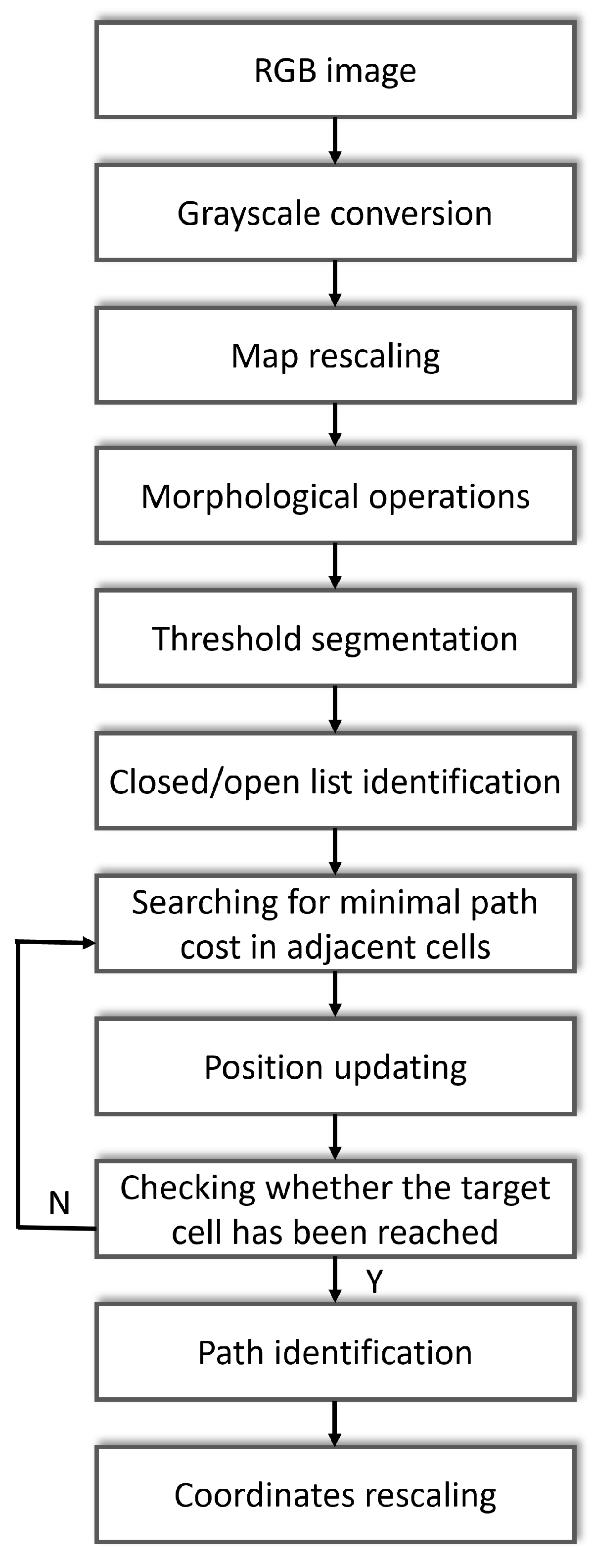
The workflow of the modified A* algorithm is presented in Figure 1. In the first step, the map size is reduced using the bicubic interpolation method depending on the entered value of the scaling factor. In this case, the scaling factor was set to 0.2 (the result image resolution is five times lower than the original). Then, morphological operations such as dilation and closing are performed with a square structuring element with dimensions of 4 × 4 pixels. After performing the above processing, the algorithm divides the environment into individual cells of a fixed size. Based on the threshold segmentation, an occupancy grid is created, providing information about each cell’s obstacle presence. In the next step, two lists are created: closed and open. The coordinates of cells containing obstacles are saved to the closed list and the rest to the open list. The algorithm starts from the starting point and adds it to the open list. In the further part of the algorithm, based on the formula presented above, , , and are calculated for each cell adjacent to the starting cell. The position is updated based on the lowest value. After this step, is recalculated for the new position’s adjacent cells. If the destination node has been reached, its coordinates are included in the open list, and there is a collision-free path from the starting point, the algorithm ends by returning the path in the form of coordinates of subsequent cells. The path is generated from the last cell, identifying parent cells, until the starting point is reached. The resulting coordinates are then scaled to the original map size according to the scaling factor.
2.2. Artificial Potential Field
The artificial potential field algorithm proposed in [41] assumes the presence of a repulsive field around the obstacle and an attractive field around the target, which influences the moving autonomous underwater vehicle. As a result of the overlap of these virtual fields, the resultant force is determined, defining the vehicle’s direction of movement. The vehicle path is created based on the subsequent coordinates of the vehicle’s movement in the presence of artificial fields towards the target. The critical aspect of the method is the accurate detection of the obstacles and the determination of the target.
The first step of the algorithm is the initialisation of the starting and destination points and map. Then, the map is binarised using threshold segmentation, as a result of which obstacles are marked with the value 1 and pixels containing free space are marked with the value 0. In the next step, the potential matrix of the repulsive field is determined as follows:
where:
- x—an analysed point on the map;
- —repulsive factor;
- —distance to the nearest obstacle (Euclidean);
- —safety distance (from the obstacle’s boundary).
The force of the repulsive field is calculated through the gradient as follows:
where:
- —coordinates of the obstacle.
Then, the potential matrix of the attracting field is determined:
where:
- —attractive factor,
- —target coordinates.
Similarly to the repulsive force, the attractive force is calculated as a gradient as follows:
The total value of the force acting on the vehicle is expressed as the sum of the attractive force and repulsive force gradients:
The coordinates of the next point are calculated using the following relationship:
where:
- —last calculated point in the path;
- —total force acting on the vehicle in the analysed point.
The algorithm stops when the following condition is met:
where:
- —specific threshold expressing tolerance of reaching the goal coordinates.
The calculated path is returned as successive coordinates connecting the starting and ending points. The method has a low computational cost and is easy to implement, which allows it to be used in vehicles operating and making decisions in close to real time. Despite the above advantages, the algorithm is sensitive to the occurrence of local minima and situations in which the shape of the obstacle creates a trap (e.g., a U-shaped obstacle) [42]. In this case, the force acting on the vehicle is balanced and the algorithm will control the vehicle’s motion in a closed infinite loop without achieving the goal. Additionally, travelling between obstacles close to each other may not be possible or cause path oscillations caused by the alternating influence of oppositely directed fields coming from the obstacles [42,43]. Moreover, in this method, the vehicle usually tends to have unstable movements when avoiding obstacles.
2.3. Genetic Algorithm
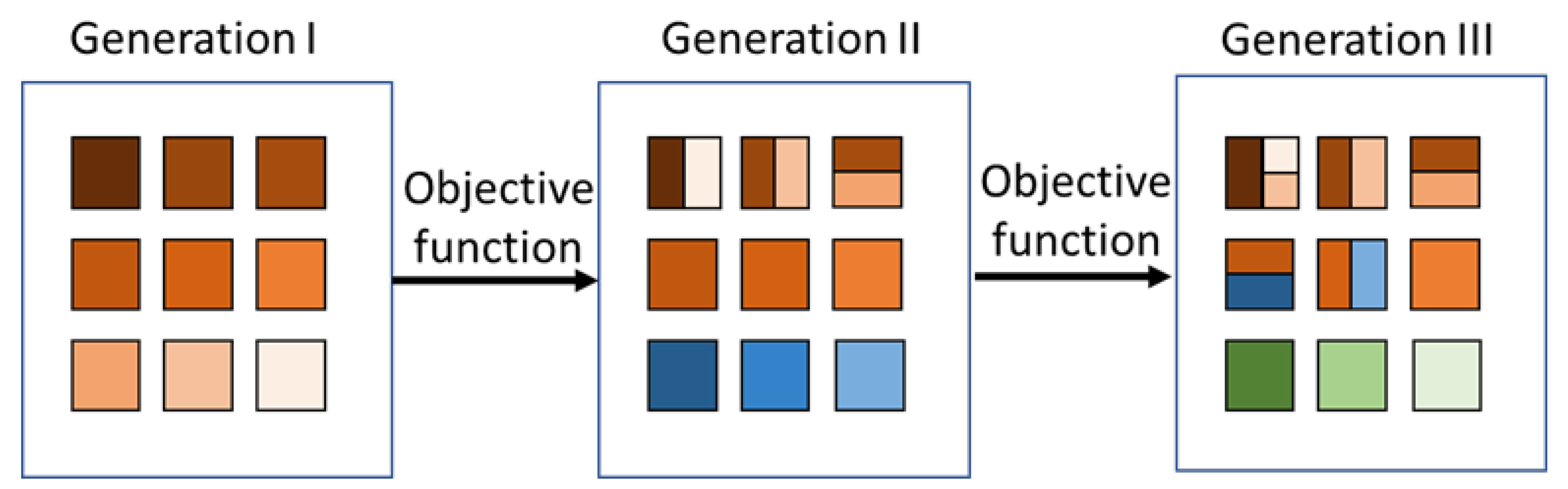
Genetic algorithm (GA) refers to an optimisation method inspired by the natural process of evolution, in which only the best-adapted organisms have a chance to survive. The search for a solution to a problem begins by generating a random population of possible solutions. Depending on the used cost function, a selection is made, during which the least suitable solutions are eliminated. For path planning, the main criterion is the path cost. Then, through the operation of crossover, i.e., combining the parents’ genotypes, further potential solutions to the problem (offspring) are created, combining the best solutions of the previous generation (parents). The best solutions are also replicated in the new generation. Additionally, the mutation process creates random modifications of the best solutions. The GA then performs the selection again, adding further possible solutions to the population that are closer and closer to the optimal result. This process is repeated until a specific end condition is reached, e.g., the number of generations. The abovementioned idea of the algorithm is presented in Figure 2.
The cost function used in this research is presented below:
where:
- k—number of the current waypoint;
- m—total number of waypoints;
- —Euclidean distance between the successive waypoints, calculated as:
- n—number of the following path segments between the successive waypoints;
- —length of the i-th path segment expressed as follows:
—penalty for path calculation through the obstacle expressed as follows:
In the initial phase of the algorithm, the coordinates of the starting and destination points and the map in a binarised form are loaded, depending on the segmentation threshold. Then, the initial parameters of the GA method are introduced. The basic parameters and their initial values are presented below:
- number of calculated points between the start and end points—2 (in the form of , and , );
- number of generations—10;
- population size—5000 individuals;
- the number of individuals (paths) guaranteed to survive to the next generation—0.05;
- mutation rate probability—0.01;
- fraction of each population, other than elite children, that is made up of crossover children—0.8;
- number of points after interpolation—100 points.
Later in the algorithm, Matlab’s “ga” function is used, an element of the “Global Optimization Toolbox”. The objective function specifies the high penalty value for determining the path using the coordinates where the obstacles are located (with a 1-pixel checking resolution). Based on the previously defined GA parameters and the objective function, two intermediate points are determined between the start and the target. Then, the path is supplemented with additional intermediate points as a result of interpolation. The more points are analysed, the better results are provided by the algorithm. It depends primarily on the number of populations and the number of generations. However, this leads to increased computational costs.
2.4. Particle Swarm Optimisation
The method refers to the behaviour observed among animals moving in groups (e.g., flocks of birds). Searching for optimal solutions consists of examining space by a population of particles. The movement of each particle depends on the best result obtained in previous iterations, the best result of the entire swarm, and a random value. In each subsequent iteration, the results of each particle are evaluated based on the objective function, and the group score is updated, which results in the gradual focusing of each particle around the best solutions. The most important parameters used in simulation:
- number of calculated points between the start and end points—2 (in the form of , and , );
- swarm size—3000 particles;
- max stall iterations (ending condition), which is the specified number of iterations during which the change in best objective function value does not exceed the tolerance value—8 iterations;
- tolerance value of changes in the best objective function that is used to stop the algorithm—;
- upper and lower bound for solution—map size [pixels], map size [pixels];
- each particle’s best position weight in velocity calculations—1.49;
- neighbourhood’s best position weight in velocity calculations—1.49;
- inertia coefficient regulating the impact of the current particle speed on the particle’s speed in the next iteration—adaptive value in the range of 0.1–1.1;
- number of points after interpolation—100 points.
The algorithm takes a subset with a specific number of particles (paths) in the form of vectors of coordinates of intermediate points between the start and the target. Then, each particle is analysed using the objective function. The objective function used in this algorithm is the same as in GA (Equations (9)–(11)). Based on the results of the above analysis, the particle movement velocity is updated to find the best solution according to the following formula [44]:
where:
- x—analysed position (in the form of vector of coordinates considered as potential solutions);
- w—inertia coefficient;
- —velocity in a previous iteration [pixels/iteration];
- —uniformly distributed random factors;
- — each particle’s best position weight;
- —neighbourhood’s best position weight;
- p—best position of an individual particle (in the form of vector of coordinates);
- g—global best position (in the form of vector of coordinates).
Then, based on the velocity, the position of each particle is updated as follows:
After updating the position, if any of the points calculated in subsequent iterations exceed the map boundary, its position is enforced at the map boundary point. Additionally, if the particle’s velocity indicates that any point will be outside the map, the particle’s velocity is set to 0. Then, the updated solutions are checked by using the objective function again. If the evaluated solution gives a better result (shorter path) than the previous one for a given particle, then p = x. A similar check is carried out for the neighbourhood. If no particle obtains a better result in a given iteration than the best global value (including tolerance value), the stall counter value increases. The algorithm is stopped when the counter value achieves the value set as the end condition. Based on the above algorithm, two intermediate points are determined between the start and the target. As a result of interpolation, additional points are added to increase the resolution of the path.
2.5. Rapidly-Exploring Random Tree
Rapidly-exploring random tree is an algorithm based on expanding a tree composed of random edges and vortexes with a given step in search space. As the tree’s root, the starting point is considered. The next vortex is determined towards a randomly selected point in the search space with a specific step. Then, the next point in the search space is randomly selected and the nearest vortex to this point is identified. From the vortex, based on a given step, in the determined point direction, a new edge is set and the new vortex is connected to the tree. In this way, subsequent vortexes are selected until the target coordinates are reached. An example of the algorithm’s path-planning result is shown in Figure 3.
The subsequent stages of operation of the algorithm used in the global trajectory planner are described below:
- Load the starting point, destination point and map.
- Binarization of the map as a result of threshold segmentation.
- Determining the conditions for stopping the algorithm:
- checking whether the last added vortex coordinates are equal to the target point;
- checking whether the number of iterations exceeds 25,000.
- Selecting a random point on the map.
- Finding the closest tree’s vortexes based on Euclidean distance.
- Determine a point 1 pixel away from the nearest point in the tree towards a random point.
- Checking whether the analysed point is occupied.
- Checking whether the analysed point has not been previously added to the tree.
- If the analysed point is not located on an obstacle and is not part of the tree, it is added as another vortex in the tree.
- If the last added point corresponds to the target point, the algorithm determines the shortest path of subsequent nodes between the start and the target. If not, another random point is selected in the search space to determine the next potential node in the tree.
Since the algorithm does not check all points in space, it allows for quickly finding a path between the start and the destination if such a path exists. The disadvantage of the algorithm is that the calculated path may not be optimal in terms of length.
3. Multimodal Global Trajectory Planner
Based on extensive literature analysis [45], the most promising path-planning methods were selected, demonstrating the high effectiveness of collision avoidance systems for AUVs/ASVs. Due to their disadvantages, the methods described above are often combined with other methods to avoid the negative impact of the drawbacks of each method on the final effect of path planning [14,23,36,46]. However, some problems are revealed only in specific conditions, such as trap obstacles shape (U shape or V shape), almost closed obstacles (small entrance isthmus), obstacles located at a very short distance from each other, a large number of complex irregular obstacles occurring between the starting and ending points and the high dimensionality of the path planning map. Therefore, choosing the appropriate method to use in a global trajectory planning system is very difficult. The presented approach avoids these shortcomings by simultaneously determining the path using different methods. The general workflow of the system is shown in Figure 4.
The detailed principle of the system’s operation is presented below:
- Entering the geographical coordinates of subsequent waypoints in the order in which the vehicle is intended to move. The entered coordinates are converted from the geographical reference system to the local reference system resulting from reading the satellite image as an RGB image. Each waypoint is assigned to the appropriate pixel in the image. In this way, the path to be determined by the global trajectory planning system is divided into segments.
- Map initialisation, image processing and threshold segmentation to determine the occupancy grid. Then, checking the entered starting position, subsequent waypoints and the target position of the vehicle in terms of accessibility is conducted.
- Calculating 5 paths in the form of a set of pixels for each segment, using different methods with parallel processing.
- Checking whether intermediate points in the local coordinate system with a step of 1 pixel between adjacent waypoints do not contain obstacles and whether the last point of the designated path is within a radius of 20 pixels from the target.
- Calculation of the path length in geographical coordinates, considering the World Geodetic System of 1984 (WGS84) as a reference ellipsoid. The path is calculated between subsequent geographical coordinates resulting from converting the position of subsequent pixels on the map image into longitude and latitude. The distance cost between adjacent waypoints in each segment is assigned to a set of geographic coordinates representing the designated path for each method.
- Selection of the shortest path in individual segments.
- Synthesis of the paths based on individual segments with information on the distance cost for each intermediate point.
- Determining the final trajectory based on the average speed of the vehicle (this parameter may have different values depending on the type of the vehicle, its physical parameters, propulsion, etc.—therefore, it is assumed that the average speed of the vehicle will be defined by the user based on knowledge about the actual parameters of the vehicle). In this case, in order to simplify the calculations, the value of 1 m/s was adopted. Since the final trajectory includes information about the distance travelled from the starting point, the times of reaching individual path points can be calculated taking into account kinematic constraints. The trajectory is determined by calculating arrival times and assigning them to all coordinates in the synthesised path.
Since the input information (coordinates of the starting, intermediate and end points) is entered in geographical coordinates, and the output trajectory is expressed in geographical coordinates, the planner is a practical tool for use in real solutions, both AUVs and ASVs equipped with trajectory tracking control system [47]. Proper system operation requires prior preparation of the map to separate obstacles (terrain) from the free space. This can be done based on any map in geographical coordinates that isolate the area occupied by obstacles and available for vehicle movement. It is worth noting that using the above-described system in a dynamic port environment does not provide full protection against collisions between obstacles and the vehicle. The system can only be used for static obstacles. However, collision avoidance in relation to dynamic obstacles is most often realised by a local collision avoidance system which requires cooperation with an obstacle detection system [48]. Therefore, to ensure the safe execution of the trajectory planned by the multimodal global trajectory planner in a dynamic environment, it is necessary to equip the AUV with at least a reactive local collision avoidance system (e.g., implementing momentary course changes in the event of an obstacle in front of the vehicle), which determines equipping of the AUV with an additional sensor for environmental detection e.g., echosounder [49].
4. Simulation Research
To evaluate the presented planner’s capabilities the map of an environment close to the real one [50] was prepared. The assumption was that the environment expressed by the map would represent a place where the AUVs/ASVs can operate in challenging conditions, and the path to be determined by the global trajectory planner would be difficult in terms of planning. An additional assumption was to consider a large planning area to verify the planner’s functionality in terms of implementation in real underwater systems. To meet the above assumptions, a satellite map of the Port of Gdynia (Poland) and Port of Livorno (Italy) after image processing was used, where the vehicle could perform patrol functions, supervise the space or inspect specific places in the port or near the port entrance in the event of intruders (sabotaging AUVs, divers, etc.) as well as an enemy vehicle imitator to test port security. Preparing the map for use in the global planner is shown in Figure 5.
Based on the satellite map reading as an RGB image using the Mapping Toolbox in the Matlab environment, an image consisting of 4 fragments of satellite images of the ports in Gdynia and Livorno were created to obtain a high-resolution input map. The resulting images resolution were 4015 × 3884 pixels (Gdynia) and 2144 × 1359 pixels (Livorno), where one pixel represents a real area of approximately 1.3862 × 1.3891 m and 3.4631 × 3.4637 m, respectively.
The next step in preparing the map was to transform the image presented in the form of the RGB system to grayscale in accordance with the following relationship [44]:
where:
- R, G, B—red, green, and blue colour components (respectively) expressed in the range of 0–255.
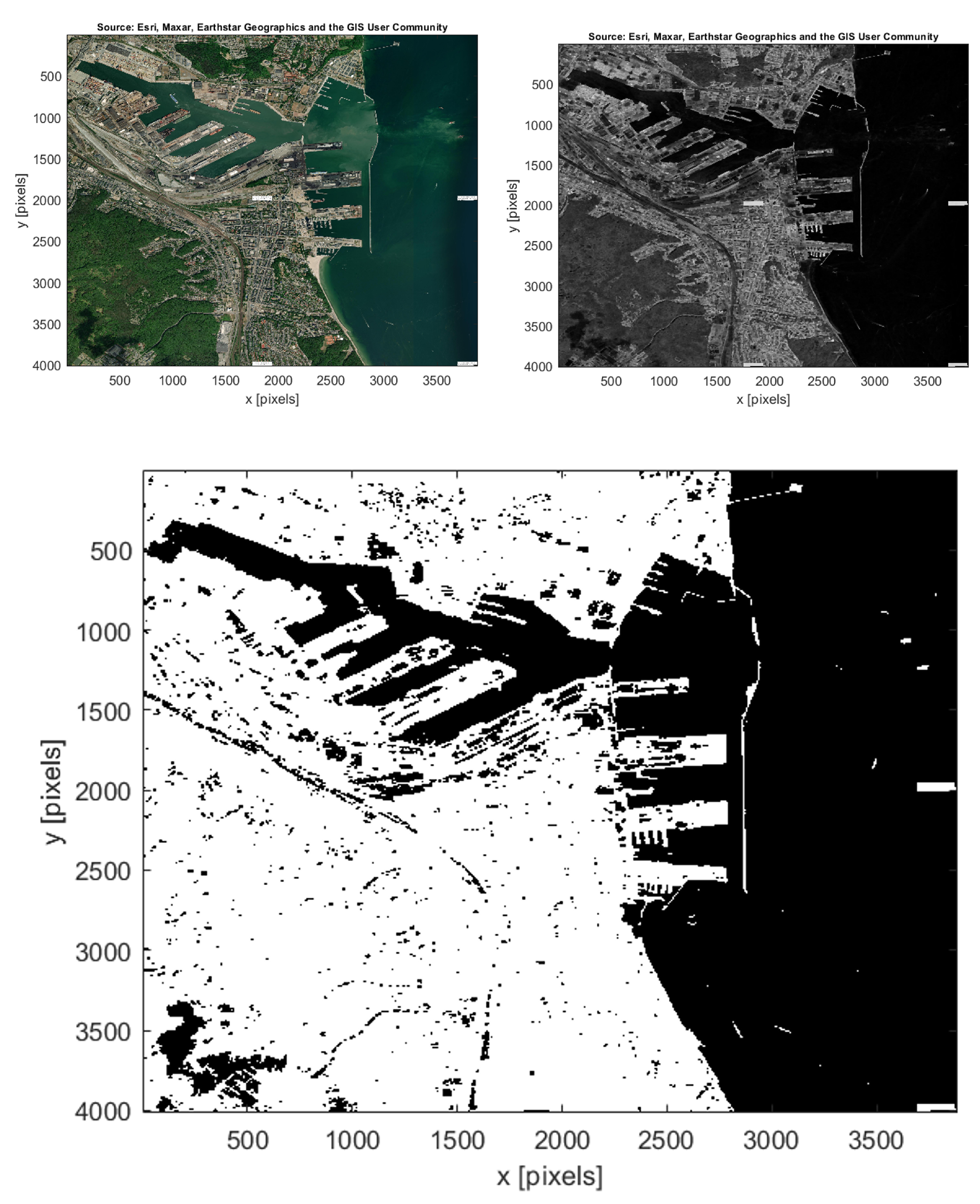
To better separate occupied space (terrain) from free space (water), mathematical morphology operations were used: first, a top-hat transformation with a structural element in the form of a square with dimensions of 25 × 25 pixels, and then a closing operation with a structural element in the form of a square with dimensions of 10 × 10 pixels. Threshold segmentation operation was used to binarise the grayscale map. Subsequent stages of map image processing for the port of Gdynia are presented in Figure 6. Exactly the same processing order with identical parameters was applied to the map of the port of Livorno.
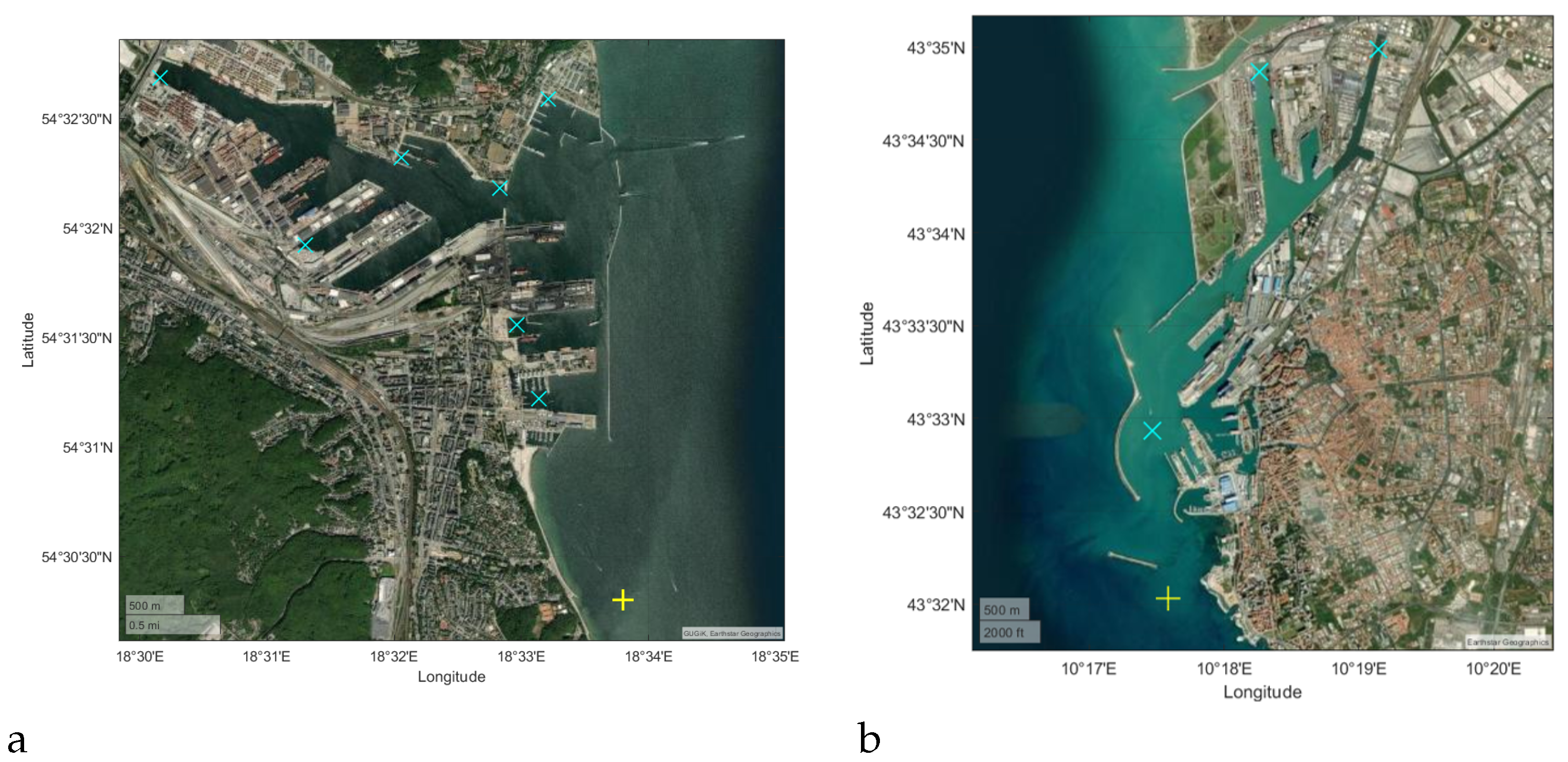
The threshold value was selected experimentally to obtain the best area occupancy results in relation to the real image, and the set value was 35/255. This means that if the pixel brightness expressed on a scale from 0–255 is more than 35, the analysed pixel is treated as occupied (an area inaccessible to the vehicle—containing an obstacle). If the pixel value is less than or equal to the segmentation threshold value, the area expressed by the analysed pixel is treated as available space for path planning (does not contain an obstacle). Based on the representation of the port area created in this way, the global planner approach described in the previous section was tested in terms of determining a path expressed in 9 waypoints (8 segments) in case of the port of Gdynia and 5 waypoints (4 segments) in case of the port of Livorno. Each waypoint was selected in such a way as to check global planner’s performance in determining both simple and complex situations. The location of waypoints is shown in Figure 7.
In case of AUVs, the study assumes that the vehicle operates at a constant depth of 3 m in case of the port of Gdynia and 1.5 m in case of the port of Livorno. The assumption is connected to the minimum depths of the areas of the water reservoir in which the AUV operates. An overview map with the Port of Gdynia depth distribution can be found in reference [51].
5. Results and Analysis
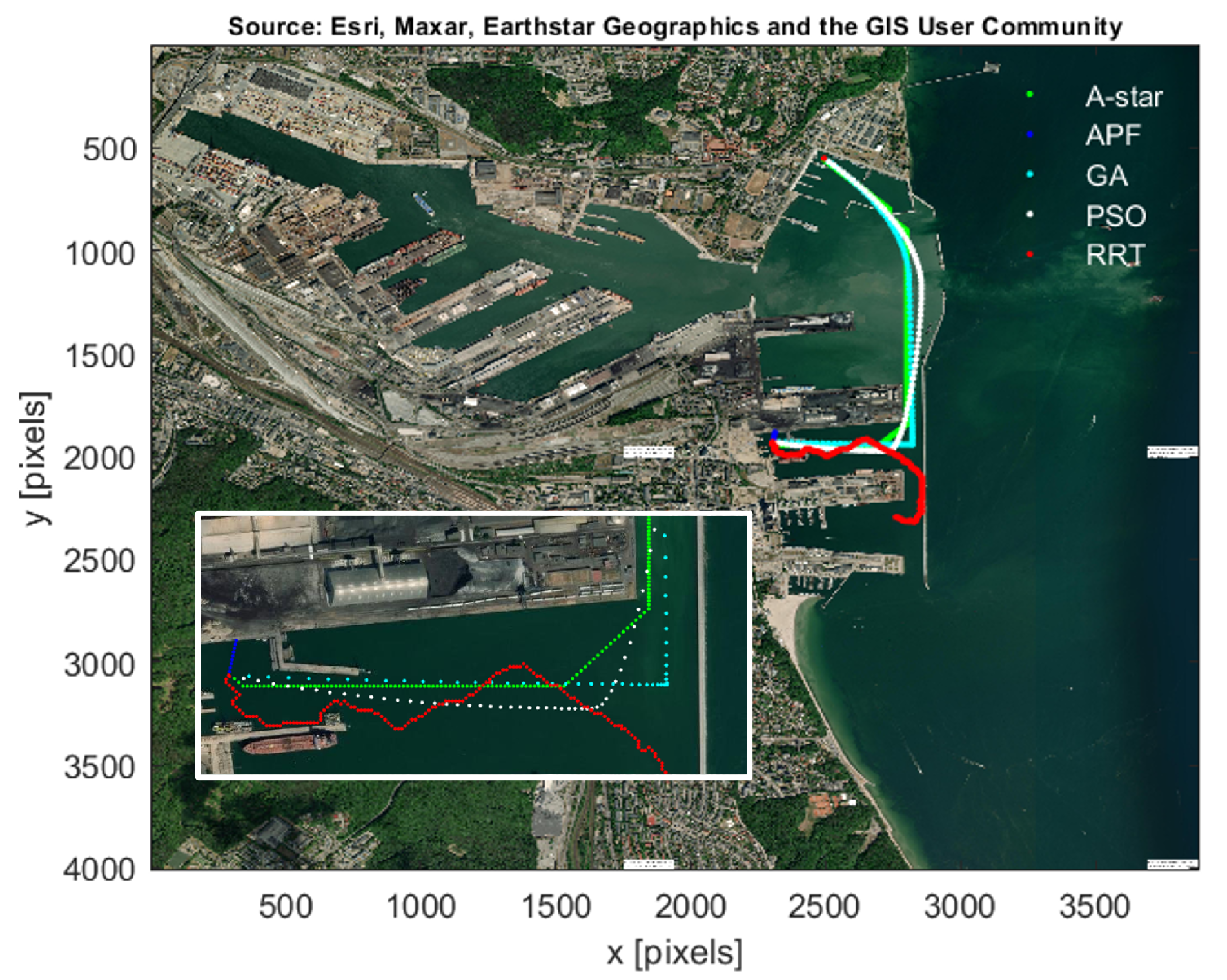
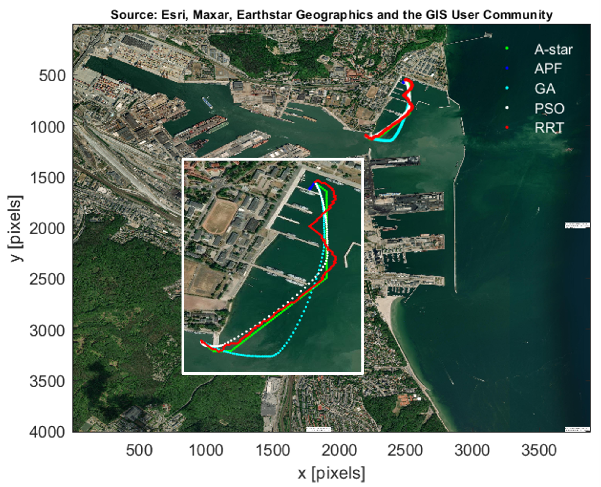
In order to verify the effectiveness of path planning by the multimodal global trajectory planner, a Matlab simulation was performed. The simulation results in the form of paths on the port of Gdynia satellite image background are presented in Figure 8, Figure 9, Figure 10, Figure 11, Figure 12, Figure 13, Figure 14 and Figure 15. The paths calculated for the port of Livorno are presented in Figure 16, Figure 17, Figure 18 and Figure 19. All resulting figures together with their Matlab source figures are available in the Supplementary Materials (S1).
The results of path planning in terms of length and computation time (Intel Core i5 10 gen, 1.60 GHz, 8 GB RAM, Win11 Home) are presented in Table 1 and Table 2 for the port of Gdynia and Table 3 and Table 4 for the port of Livorno. If the path calculation was unsuccessful (the last of the calculated points was more than 20 pixels away from the target point or the path runs through prohibited areas), the algorithm assigns the distance between waypoints in the analysed segment equal to 1,000,000 m. This prevents the algorithm from selecting a short but unfeasible path as the most effective one designated for the analysed waypoints. Based on the results obtained, it can be concluded that none of the methods fully ensures the determination of a feasible path individually in such a complicated environment as a seaport in complex situations. Since the APF and RRT methods obtained least feasible paths, the methods are the most sensitive to the complexity of the environment. This comes from the fact that the APF algorithm was used in the basic version without any improvements preventing the local minima problem. Therefore, it quickly results in finding a local minimum and making it impossible to calculate a further path. However, when the location of subsequent waypoints allows the determination of a path as a straight line or curve, APF determines the shortest path of all methods. In the case of RRT, when tuning the method’s operation, attempts were made to select the number of iterations in such a way that the calculation time for one segment was approximately 10 min. Larger values are impractical because they significantly affect the total calculation time associated with path planning. The greatest number of segments where the path has been correctly determined was achieved by modified A* algorithm and the greatest number of shortest paths were achieved by the modified A* and GA algorithms. However, modified A* was the only method that calculated a feasible path for the seventh and eighth segments in case of the port of Gdynia simulations and for the fourth segment in case of the port of Livorno. Unfeasible paths calculated by GA and PSO using the same objective function are due to too few points analysed for such a large map and to the initial assumption of determining two intermediate (“optimal”) points between the start and the goal. In cases 7 and 8 (port of Gdynia) and in case 4 (port of Livorno) calculating three “optimal” path points instead of two could effectively determine a collision-free path. However, this will significantly increase the computation time. Moreover, to achieve a near-optimal path, the population and the generation number should also be increased, which would further increase the computation time. The total path determined by the global trajectory planner was about 20 km (in case of the port of Gdynia) and about 15 km (in case of the port of Livorno), which, assuming the vehicle moves at a speed of 1 m/s, means that the entire mission will last approximately 5.5 h and 4 h, respectively.
The above analysis confirms that each used algorithm has flaws that are revealed in various situations. For example, the disadvantages related to the selection of one of the 8 pixels around the analysed pixel in each iteration of the A* algorithm and the disadvantages resulting from the approximation of the optimal path (in terms of length) by GA and PSO are revealed in particular when planning paths similar to a straight line. These disadvantages are effectively overcome by the APF algorithm because the impact of the attractive force in unobstructed spaces enforces the determination of the subsequent points in the direction of the destination point. On the other hand, in the case of very long paths with many turning points, APF disadvantages appear, such as looping the algorithm in a local minimum, and GA and PSO disadvantages resulting from the approximation of the designated path using two points (additional intermediate points result from interpolation). The above disadvantages are overcome by modified A*, which, in the case of long routes, ensures effective path determination regardless of the number of turning points. However, for long and short paths with small number of turning points, better results are usually obtained using GA or PSO. The disadvantages of RRT are visible in each case examined and include a sub-optimal path length, even on short and medium segments (less than 2–3 km), and long-term calculations to find a path between the starting and ending points for a large map (like the maps used in this study). Increasing the allowable number of iterations would make it possible to determine the path in every case (if a feasible path exists). However, in this study, the number of iterations was limited for practical reasons, which, in most cases, makes the calculated path unfeasible. The above method was retained to increase the reliability of path planning when the mission planning time is not important.
Based on the calculation time results in Table 2 and Table 4, it can be concluded that the length of the path in a given segment and its complexity do not affect the calculation time in the APF, GA and PSO methods. However, in the APF method, the calculation time was very short (about 1–2 s) and in the GA and PSO methods relatively long (a few minutes). On the other hand, the path obtained using APF was feasible in only 1 case, while for the GA and PSO methods, the path was feasible in 6 and 5 cases, respectively, in case of the port of Gdynia and in 3 and 1 segments for the port of Livorno simulations. The most significant differences in calculation time are noticeable in the RRT method. The calculation took about 1 s in two cases and two others over 10 min. From the entire system’s point of view, the longest computation time for each segment determines the total computation time. Despite using parallel processing for all methods, the total calculation time was approximately 1 h for path planning in the port of Gdynia and about 30 min in case of the port of Livorno. Long computation time is connected with the mission’s high complexity level. Processing, e.g., 8 segments in parallel would cut the time in half but requires additional processor cores and limits the number of waypoints entered to the number of available processor cores. Despite the relatively large calculation time, which is acceptable at the stage of planning a mission with the presented level of complexity, the determined trajectory is feasible, almost optimal in terms of the distance and automatically calculated.
It is also worth noting that in the case of such a complicated environment, using only one method would not allow for obtaining the entire collision-free trajectory. As a result of the multimodal global planner, a trajectory is obtained in the form of a set of geographical coordinates, distance cost and arrival times. The final paths are shown in Figure 20, which confirms the correct operation of the global trajectory planner in a complex port environment. Additionally, since the final trajectory is expressed in the form of longitude and latitude, it can be easily implemented in vehicles with a trajectory tracking system. Currently, many AUVs used commercially or in the military are equipped with such a system. Therefore, there is a great chance of applying the results of this research in relation to real vehicles. The use of a global trajectory planning system based on several path planning methods allows obtaining the advantage of getting a near-optimal path in terms of the distance as well as high system reliability in the case of complex situations with acceptable calculation time at the mission planning stage.
6. Conclusions
The article presents a multimodal global trajectory planner for AUVs/ASVs that uses five path planning methods in relation to a high-dimensional map of a complex environment, such as the port of Gdynia. The system proved to be effective despite the selection of challenging paths to designate. However, none of the individual methods determined the entire collision-free path (for all segments). The presented system effectively uses each method’s advantages and overcomes their shortcomings. Based on the results presented in Figure 8, Figure 9, Figure 10, Figure 11, Figure 12, Figure 13, Figure 14, Figure 15, Figure 16, Figure 17, Figure 18 and Figure 19 it can be concluded that the APF method is effective for planning simple paths close to a straight line. Very complicated and long paths are best calculated using modified A*. GA and PSO are effective for long and short paths that do not require many turning points. The RRT algorithm increases the system’s reliability, assuming that the path planning time is not an important factor. Based on Table 1 and Table 3, most of the shortest path segments were obtained by modified A* and GA. In terms of calculation time, based on the results in Table 2 and Table 4, the APF and modified A* methods achieved the shortest time. The use of several computational methods in the system allows both to select an almost optimal path and also to increase the reliability of path determination. Additionally, regarding path length, better results have been obtained by the global trajectory planning system than the paths calculated for all segments by each method individually. This confirms the effectiveness of the system and its purposefulness. Proposed approach was tested in two different port areas. In both cases the system was calculated a feasible trajectory and proves the effectiveness and robustness of not only the algorithms used but also the method of processing the satellite map to create an environment capable of being used in the path planning process. Expressing the final trajectory in the form of geographical coordinates with a specific arrival time allows the implementation of calculation results in mission planning for underwater vehicles used commercially and in the military, e.g., in Hugin or Gavia vehicles, as well as for ASVs equipped with trajectory tracking systems. The integration of the proposed approach with other systems depends on the individual vehicle’s mission planning system as well as high and low-level control systems. Commercial systems usually provide software that allows mission planning by entering trajectories expressed in geographic coordinates and corresponding arrival times in text form. Some AUV manufacturers offer mission simulators in which the trajectory can be verified for a specific vehicle. Since the proposed approach does not take into account path smoothing and sharp turns optimisation (which may occur when combining trajectories from individual segments), it should be taken into account that in the above situations, the vehicle may behave unpredictably depending on the operation of the trajectory tracking control system. Future works will include adding algorithms for path smoothing and sharp turns optimising, as well as verifying the calculated trajectory in an AUV simulation model equipped with a trajectory tracking control system and a local collision avoidance system in a dynamic environment.
Supplementary Materials
The following supporting information can be downloaded at: https://figshare.com/articles/figure/Multimodal_global_trajectory_planner_-_results/24416512.
Funding
This research received no external funding.
Institutional Review Board Statement
Not applicable.
Informed Consent Statement
Not applicable.
Data Availability Statement
Data are contained within the article and Supplementary Materials.
Acknowledgments
The author would like to thank Piotr Szymak and Paweł Piskur for their mentorship, support, and motivation in his academic and personal development.
Conflicts of Interest
The authors declare no conflict of interest.
Abbreviations
The following abbreviations are used in this manuscript:
| APF | Artificial Potential Field |
| ASVs | Autonomous Surface Vehicles |
| AUVs | Autonomous Underwater Vehicles |
| DL | Deep Learning |
| FL | Fuzzy Logic |
| GA | Genetic Algorithm |
| NN | Neural Networks |
| PSO | Particle Swarm Optimisation |
| RL | Reinforcement Learning |
| RRT | Rapidly-exploring Random Tree |
References
- Kot, R.; Szymak, P. Fine-Tuning Method of the GA-based Collision Avoidance System for AUVs. In Proceedings of the 2023 27th International Conference on Methods and Models in Automation and Robotics (MMAR), Miedzyzdroje, Poland, 22–25 August 2023; pp. 400–405. [Google Scholar]
- Cheng, C.; Zhu, D.; Sun, B.; Chu, Z.; Nie, J.; Zhang, S. Path planning for autonomous underwater vehicle based on artificial potential field and velocity synthesis. In Proceedings of the 2015 IEEE 28th Canadian Conference on Electrical and Computer Engineering (CCECE), Halifax, NS, Canada, 3–6 May 2015; pp. 717–721. [Google Scholar]
- Solari, F.J.; Rozenfeld, A.F.; Villar, S.A.; Acosta, G.G. Artificial potential fields for the obstacles avoidance system of an AUV using a mechanical scanning sonar. In Proceedings of the 2016 3rd IEEE/OES South American International Symposium on Oceanic Engineering (SAISOE), Buenos Aires, Argentina, 15–17 June 2016; pp. 1–6. [Google Scholar]
- Williams, G.N.; Lagace, G.E.; Woodfin, A. A collision avoidance controller for autonomous underwater vehicles. In Proceedings of the Symposium on Autonomous Underwater Vehicle Technology, Washington, DC, USA, 5–6 June 1990; pp. 206–212. [Google Scholar]
- Barišić, M.; Vukić, Z.; Mišković, N. A kinematic virtual potentials trajectory planner for AUV-s. IFAC Proc. Vol. 2007, 40, 90–95. [Google Scholar] [CrossRef]
- Braginsk, B.; Karabchevsk, S.; Guterma, H. Two layers obstacle avoidance algorithm for autonomous underwater vehicle. In Proceedings of the 2012 IEEE 27th Convention of Electrical and Electronics Engineers in Israel, Eilat, Israel, 14–17 November 2012; pp. 1–5. [Google Scholar]
- Karabchevsky, S.; Braginsky, B.; Guterman, H. AUV real-time acoustic vertical plane obstacle detection and avoidance. In Proceedings of the 2012 IEEE/OES Autonomous Underwater Vehicles (AUV), Southampton, UK, 24–27 September 2012; pp. 1–6. [Google Scholar]
- Subramanian, S.; George, T.; Thondiyath, A. Hardware-in-the-Loop verification for 3D obstacle avoidance algorithm of an underactuated flat-fish type AUV. In Proceedings of the 2012 IEEE International Conference on Robotics and Biomimetics (ROBIO), Guangzhou, China, 11–14 December 2012; pp. 545–550. [Google Scholar]
- Horner, D.P.; Healey, A.J.; Kragelund, S.P. AUV experiments in obstacle avoidance. In Proceedings of the OCEANS 2005 MTS/IEEE, Washington, DC, USA, 17–23 September 2005; pp. 1464–1470. [Google Scholar]
- Yan, Z.; Li, J.; Jiang, A.; Wang, L. An Obstacle Avoidance Algorithm for AUV Based on Obstacle’s Detected Outline. In Proceedings of the 2018 37th Chinese Control Conference (CCC), Wuhan, China, 25–27 July 2018; pp. 5257–5262. [Google Scholar]
- Liu, Y.; Liu, L.; Yu, X.; Wang, C. Optimal Path Planning Algorithm of AUV State Space Sampling Based on Improved Cost Function. In Proceedings of the 2020 39th Chinese Control Conference (CCC), Shenyang, China, 27–29 July 2020; pp. 3747–3752. [Google Scholar]
- Yan, Z.; Li, J.; Wu, Y.; Yang, Z. A novel path planning for AUV based on objects’ motion parameters predication. IEEE Access 2018, 6, 69304–69320. [Google Scholar] [CrossRef]
- McMahon, J.; Plaku, E. Mission and motion planning for autonomous underwater vehicles operating in spatially and temporally complex environments. IEEE J. Ocean. Eng. 2016, 41, 893–912. [Google Scholar] [CrossRef]
- Qiu, X.; Feng, C.; Shen, Y. Obstacle avoidance planning combining reinforcement learning and RRT* applied to underwater operations. In Proceedings of the OCEANS 2021: San Diego–Porto, San Diego, CA, USA, 20–23 September 2021; pp. 1–6. [Google Scholar]
- Hernández, J.D.; Vidal, E.; Vallicrosa, G.; Galceran, E.; Carreras, M. Online path planning for autonomous underwater vehicles in unknown environments. In Proceedings of the 2015 IEEE International Conference on Robotics and Automation (ICRA), Seattle, WA, USA, 26–30 May 2015; pp. 1152–1157. [Google Scholar]
- Hernández, J.D.; Vidal, E.; Moll, M.; Palomeras, N.; Carreras, M.; Kavraki, L.E. Online motion planning for unexplored underwater environments using autonomous underwater vehicles. J. Field Robot. 2019, 36, 370–396. [Google Scholar] [CrossRef]
- Eichhorn, M. An obstacle avoidance system for an autonomous underwater vehicle. In Proceedings of the 2004 International Symposium on Underwater Technology (IEEE Cat. No. 04EX869), Taipei, Taiwan, 20–23 April 2004; pp. 75–82. [Google Scholar]
- Casalino, G.; Turetta, A.; Simetti, E. A three-layered architecture for real time path planning and obstacle avoidance for surveillance USVs operating in harbour fields. In Proceedings of the Oceans 2009-Europe, Bremen, Germany, 11–14 May 2009; pp. 1–8. [Google Scholar]
- Li, J.H.; Lee, M.J.; Park, S.H.; Kim, J.G. Real time path planning for a class of torpedo-type AUVs in unknown environment. In Proceedings of the 2012 IEEE/OES Autonomous Underwater Vehicles (AUV), Southampton, UK, 24–27 September 2012; pp. 1–6. [Google Scholar]
- Sun, Y.; Yang, J.; Zhao, D.; Shu, Y.; Zhang, Z.; Wang, S. A Global Trajectory Planning Framework Based on Minimizing the Risk Index. Actuators 2023, 12, 270. [Google Scholar] [CrossRef]
- Kappagantula, S.; Ramadass, G.; Adlinge, S.D. Design of a biomimetic robot fish for realization of coefficient of drag with control architecture and fuzzy logic algorithm for autonomous obstacle avoidance. In Proceedings of the 2018 3rd International Conference for Convergence in Technology (I2CT), Pune, India, 6–8 April 2018; pp. 1–9. [Google Scholar]
- Zhu, D.; Yang, Y.; Yan, M. Path planning algorithm for AUV based on a Fuzzy-PSO in dynamic environments. In Proceedings of the 2011 Eighth International Conference on Fuzzy Systems and Knowledge Discovery (FSKD), Shanghai, China, 26–28 July 2011; Volume 1, pp. 525–530. [Google Scholar]
- An, R.; Guo, S.; Zheng, L.; Hirata, H.; Gu, S. Uncertain moving obstacles avoiding method in 3D arbitrary path planning for a spherical underwater robot. Robot. Auton. Syst. 2022, 151, 104011. [Google Scholar] [CrossRef]
- Lim, H.S.; King, P.; Chin, C.K.; Chai, S.; Bose, N. Real-time implementation of an online path replanner for an AUV operating in a dynamic and unexplored environment. Appl. Ocean. Res. 2022, 118, 103006. [Google Scholar] [CrossRef]
- Gore, R.; Pattanaik, K.; Bharti, S. Efficient re-planned path for autonomous underwater vehicle in random obstacle scenario. In Proceedings of the 2019 IEEE 5th International Conference for Convergence in Technology (I2CT), Pune, India, 29–31 March 2019; pp. 1–5. [Google Scholar]
- Li, W.; Yang, X.; Yan, J.; Luo, X. An obstacle avoiding method of autonomous underwater vehicle based on the reinforcement learning. In Proceedings of the 2020 39th Chinese Control Conference (CCC), Shenyang, China, 27–29 July 2020; pp. 4538–4543. [Google Scholar]
- Guerrero-González, A.; García-Córdova, F.; Gilabert, J. A biologically inspired neural network for navigation with obstacle avoidance in autonomous underwater and surface vehicles. In Proceedings of the OCEANS 2011 IEEE-Spain, Santander, Spain, 6–9 June 2011; pp. 1–8. [Google Scholar]
- Chu, Z.; Zhu, D. Obstacle Avoidance Trajectory Planning and Trajectory Tracking Control for Autonomous Underwater Vehicles. In Proceedings of the 2018 13th World Congress on Intelligent Control and Automation (WCICA), Changsha China, 4–8 July 2018; pp. 450–454. [Google Scholar]
- Xu, H.; Feng, X. An AUV fuzzy obstacle avoidance method under event feedback supervision. In Proceedings of the OCEANS 2009, Bremen, Germany, 11–14 May 2009; pp. 1–6. [Google Scholar]
- Fodrea, L.R.; Healey, A.J. Obstacle avoidance control for the REMUS autonomous underwater vehicle. IFAC Proc. Vol. 2003, 36, 103–108. [Google Scholar] [CrossRef]
- Wu, X.; Feng, Z.; Zhu, J.; Allen, R. Line of sight guidance with intelligent obstacle avoidance for autonomous underwater vehicles. In Proceedings of the OCEANS 2006, Boston, MA, USA, 18–22 September 2006; pp. 1–6. [Google Scholar]
- Galarza, C.; Masmitja, I.; Prat, J.; Gomaríz, S. Design of obstacle detection and avoidance system for Guanay II AUV. In Proceedings of the 2016 24th Mediterranean Conference on Control and Automation (MED), Athens, Greece, 21–24 June 2016; pp. 410–414. [Google Scholar]
- Li, X.; Wang, W.; Song, J.; Liu, D. Path planning for autonomous underwater vehicle in presence of moving obstacle based on three inputs fuzzy logic. In Proceedings of the 2019 4th Asia-Pacific Conference on Intelligent Robot Systems (ACIRS), Nagoya, Japan, 13–15 July 2019; pp. 265–268. [Google Scholar]
- Chang, Z.H.; Tang, Z.D.; Cai, H.G.; Shi, X.C.; Bian, X.Q. GA path planning for AUV to avoid moving obstacles based on forward looking sonar. In Proceedings of the 2005 International Conference on Machine Learning and Cybernetics, Guangzhou, China, 18–21 August 2005; Volume 3, pp. 1498–1502. [Google Scholar]
- Yao, P.; Zhao, S. Three-dimensional path planning for AUV based on interfered fluid dynamical system under ocean current (June 2018). IEEE Access 2018, 6, 42904–42916. [Google Scholar] [CrossRef]
- Yan, S.; Pan, F. Research on route planning of AUV based on genetic algorithms. In Proceedings of the 2019 IEEE International Conference on Unmanned Systems and Artificial Intelligence (ICUSAI), Xi’an, China, 22–24 November 2019; pp. 184–187. [Google Scholar]
- Vibhute, S. Adaptive dynamic programming based motion control of autonomous underwater vehicles. In Proceedings of the 2018 5th International Conference on Control, Decision and Information Technologies (CoDIT), Thessaloniki, Greece, 10–13 April 2018; pp. 966–971. [Google Scholar]
- Praczyk, T. Neural collision avoidance system for biomimetic autonomous underwater vehicle. Soft Comput. 2020, 24, 1315–1333. [Google Scholar] [CrossRef]
- Yuan, J.; Wang, H.; Zhang, H.; Lin, C.; Yu, D.; Li, C. AUV obstacle avoidance planning based on deep reinforcement learning. J. Mar. Sci. Eng. 2021, 9, 1166. [Google Scholar] [CrossRef]
- Gaya, J.O.; Gonçalves, L.T.; Duarte, A.C.; Zanchetta, B.; Drews, P.; Botelho, S.S. Vision-based obstacle avoidance using deep learning. In Proceedings of the 2016 XIII Latin American Robotics Symposium and IV Brazilian Robotics Symposium (LARS/SBR), Recife, Brazil, 8–12 October 2016; pp. 7–12. [Google Scholar]
- Khatib, O. Real-time obstacle avoidance for manipulators and mobile robots. Int. J. Robot. Res. 1986, 5, 90–98. [Google Scholar] [CrossRef]
- Koren, Y.; Borenstein, J. Potential field methods and their inherent limitations for mobile robot navigation. In Proceedings of the ICRA, Sacramento, CA, USA, 9–11 April 1991; Volume 2, pp. 1398–1404. [Google Scholar]
- Teo, K.; Ong, K.W.; Lai, H.C. Obstacle detection, avoidance and anti collision for MEREDITH AUV. In Proceedings of the OCEANS 2009, Bremen, Germany, 11–14 May 2009; pp. 1–10. [Google Scholar]
- MATLAB. Version 9.13.0 (R2022b); The MathWorks Inc.: Natick, MA, USA, 2022. [Google Scholar]
- Kot, R. Review of collision avoidance and path planning algorithms used in autonomous underwater vehicles. Electronics 2022, 11, 2301. [Google Scholar] [CrossRef]
- Braginsky, B.; Guterman, H. Obstacle avoidance approaches for autonomous underwater vehicle: Simulation and experimental results. IEEE J. Ocean. Eng. 2016, 41, 882–892. [Google Scholar] [CrossRef]
- Szymak, P.; Kot, R. Trajectory Tracking Control of Autonomous Underwater Vehicle Called PAST. Pomiary Autom. Robot. 2022, 26, 17–22. [Google Scholar] [CrossRef]
- Kot, R. Review of Obstacle Detection Systems for Collision Avoidance of Autonomous Underwater Vehicles Tested in a Real Environment. Electronics 2022, 11, 3615. [Google Scholar] [CrossRef]
- Szymak, P.; Kot, R.; Batur, T. Numerical Research on the Mathematical Model of Echosounder for Distance to Bottom Measurement. J. Marit. Sci. Pomor. Fak. Kotor 2022, 23, 36–43. [Google Scholar] [CrossRef]
- Naus, K.; Szymak, P.; Piskur, P.; Niedziela, M.; Nowak, A. Methodology for the Correction of the Spatial Orientation Angles of the Unmanned Aerial Vehicle Using Real Time GNSS, a Shoreline Image and an Electronic Navigational Chart. Energies 2021, 14, 2810. [Google Scholar] [CrossRef]
- Biuro Hydrograficzne Marynarki Wojennej. Plan Portu Gdynia. 2023. Available online: https://bhmw.gov.pl/c/pages/gmi/2023/4/16napisy.jpg (accessed on 25 September 2023).
Figure 1.
Workflow of the modified A* algorithm.

Figure 2.
General principle of operation of the genetic algorithm (GA) optimisation algorithm.

Figure 3.
An example of the path calculation based on the rapidly-exploring random tree (RRT) algorithm. The map used in the above case is an occupancy grid obtained based on sonar measurements and threshold segmentation. The occupied space is marked in white. The yellow circle represents the starting point, and the green circle represents the destination point. Red lines represent connections between nodes added to the tree. The shortest path resulting from connecting nodes is marked in yellow.

Figure 4.
General workflow of the multimodal global trajectory planning system.

Figure 5.
Reference maps consisting of 4 fragments of a satellite image in order to obtain a larger zoom and higher resolution: (a) the port of Gdynia, (b) the port of Livorno. Source: Esri, Maxar, Earthstar Geographics and the GIS User Community.
Figure 5.
Reference maps consisting of 4 fragments of a satellite image in order to obtain a larger zoom and higher resolution: (a) the port of Gdynia, (b) the port of Livorno. Source: Esri, Maxar, Earthstar Geographics and the GIS User Community.

Figure 6.
Subsequent stages of creating an occupancy grid. First, the RGB image is converted to grayscale and processed using morphological operations (top-hat, closing). The last image presents a map in binary form after the threshold segmentation operation, expressing the presence of an obstacle in each pixel. Occupied pixels are marked in white, and free space is marked in black.

Figure 7.
Introduced waypoints’ locations in geographical coordinates on satellite image background of: (a) the port of Gdynia, (b) the port of Livorno. Successive waypoint arrangement has been selected to obtain a possibly high level of complexity in terms of path calculation. The starting and destination point is marked in yellow, and waypoints dividing the entire path to segments are marked in cyan. Source: Esri, Maxar, Earthstar Geographics and the GIS User Community.

Figure 8.
Paths calculated by each method between first and second waypoints (Port of Gdynia, segment 1).
Figure 8.
Paths calculated by each method between first and second waypoints (Port of Gdynia, segment 1).

Figure 9.
Paths calculated by each method between second and third waypoints (Port of Gdynia, segment 2).
Figure 9.
Paths calculated by each method between second and third waypoints (Port of Gdynia, segment 2).

Figure 10.
Paths calculated by each method between third and fourth waypoints (Port of Gdynia, segment 3).
Figure 10.
Paths calculated by each method between third and fourth waypoints (Port of Gdynia, segment 3).

Figure 11.
Paths calculated by each method between fourth and fifth waypoints (Port of Gdynia, segment 4).
Figure 11.
Paths calculated by each method between fourth and fifth waypoints (Port of Gdynia, segment 4).

Figure 12.
Paths calculated by each method between fifth and sixth waypoints (Port of Gdynia, segment 5).
Figure 12.
Paths calculated by each method between fifth and sixth waypoints (Port of Gdynia, segment 5).

Figure 13.
Paths calculated by each method between sixth and seventh waypoints (Port of Gdynia, segment 6).
Figure 13.
Paths calculated by each method between sixth and seventh waypoints (Port of Gdynia, segment 6).

Figure 14.
Paths calculated by each method between seventh and eighth waypoints (Port of Gdynia, segment 7).
Figure 14.
Paths calculated by each method between seventh and eighth waypoints (Port of Gdynia, segment 7).

Figure 15.
Paths calculated by each method between eighth and ninth waypoints (Port of Gdynia, segment 8).
Figure 15.
Paths calculated by each method between eighth and ninth waypoints (Port of Gdynia, segment 8).

Figure 16.
Paths calculated by each method between first and second waypoints (Port of Livorno, segment 1).
Figure 16.
Paths calculated by each method between first and second waypoints (Port of Livorno, segment 1).

Figure 17.
Paths calculated by each method between second and third waypoints (Port of Livorno, segment 2).
Figure 17.
Paths calculated by each method between second and third waypoints (Port of Livorno, segment 2).

Figure 18.
Paths calculated by each method between third and fourth waypoints (Port of Livorno, segment 3).
Figure 18.
Paths calculated by each method between third and fourth waypoints (Port of Livorno, segment 3).

Figure 19.
Paths calculated by each method between fourth and fifth waypoints (Port of Livorno, segment 4).
Figure 19.
Paths calculated by each method between fourth and fifth waypoints (Port of Livorno, segment 4).

Figure 20.
Merged paths calculated by global trajectory planning system in geographical coordinates: (a) for the port of Gdynia, (b) for the port of Livorno. Source: Esri, Maxar, Earthstar Geographics and the GIS User Community.
Figure 20.
Merged paths calculated by global trajectory planning system in geographical coordinates: (a) for the port of Gdynia, (b) for the port of Livorno. Source: Esri, Maxar, Earthstar Geographics and the GIS User Community.


Table 1.
The results of path planning in terms of path length for the port of Gdynia simulations. Unfeasible paths were marked in red. The shortest paths in each segment were marked in green.
Table 1.
The results of path planning in terms of path length for the port of Gdynia simulations. Unfeasible paths were marked in red. The shortest paths in each segment were marked in green.
| Path Length [m] | ||||||
|---|---|---|---|---|---|---|
| Method | APF | Modified A* | GA | PSO | RRT | |
| Segment Number | ||||||
| 1 | Unfeasible | 2218.634 | 2108.144 | 2110.966 | Unfeasible | |
| 2 | Unfeasible | 1588.138 | 1504.894 | Unfeasible | Unfeasible | |
| 3 | Unfeasible | 2721.349 | 2783.388 | 2760.091 | Unfeasible | |
| 4 | Unfeasible | 1091.328 | 1146.65 | 1029.075 | 1281.576 | |
| 5 | 868.5812 | 936.3178 | 870.4365 | 879.2176 | 1042.073 | |
| 6 | Unfeasible | Unfeasible | 1418.796 | 1337.666 | Unfeasible | |
| 7 | Unfeasible | 3233.793 | Unfeasible | Unfeasible | Unfeasible | |
| 8 | Unfeasible | 7353.398 | Unfeasible | Unfeasible | Unfeasible | |
| Number of feasible paths | 1 | 7 | 6 | 5 | 2 | |
| Total length of feasible paths [m] | 20,156.90 | |||||
Table 2.
The results of path planning in terms of computation time for the port of Gdynia simulations. Unfeasible paths were marked in red. The shortest paths in each segment were marked in green.
Table 2.
The results of path planning in terms of computation time for the port of Gdynia simulations. Unfeasible paths were marked in red. The shortest paths in each segment were marked in green.
| Calculation Time [s] | ||||||
|---|---|---|---|---|---|---|
| Method | APF | Modified A* | GA | PSO | RRT | |
| Segment Number | ||||||
| 1 | 1.4 | 227.1 | 488.6 | 246.5 | 645.2 | |
| 2 | 1.5 | 83.2 | 475.9 | 365.0 | 670.1 | |
| 3 | 1.0 | 136.8 | 309.3 | 412.7 | 305.1 | |
| 4 | 1.7 | 78.2 | 465.3 | 397.9 | 1.1 | |
| 5 | 1.7 | 112.5 | 465.3 | 301.8 | 1.2 | |
| 6 | 1.6 | 63.6 | 479.6 | 377.5 | 462.6 | |
| 7 | 1.2 | 94.9 | 512.6 | 454.0 | 47.1 | |
| 8 | 1.0 | 274.7 | 348.1 | 295.7 | 126.5 | |
| Total calculation time [s] | 11.1 | 1071.0 | 3544.6 | 2851.1 | 2258.9 | |
Table 3.
The results of path planning in terms of path length for the port of Livorno simulations. Unfeasible paths were marked in red. The shortest paths in each segment were marked in green.
Table 3.
The results of path planning in terms of path length for the port of Livorno simulations. Unfeasible paths were marked in red. The shortest paths in each segment were marked in green.
| Path Length [m] | ||||||
|---|---|---|---|---|---|---|
| Method | APF | Modified A* | GA | PSO | RRT | |
| Segment Number | ||||||
| 1 | 1686.900 | 1743.916 | 1717.055 | 1699.229 | Unfeasible | |
| 2 | Unfeasible | 4739.060 | 4566.755 | Unfeasible | Unfeasible | |
| 3 | Unfeasible | 3172.850 | 3065.002 | Unfeasible | 3643.001 | |
| 4 | Unfeasible | 5762.071 | Unfeasible | Unfeasible | Unfeasible | |
| Number of feasible paths | 1 | 4 | 3 | 1 | 1 | |
| Total length of feasible path [m] | 15,080.73 | |||||
Table 4.
The results of path planning in terms of computation time for the port of Livorno simulations. Unfeasible paths were marked in red. The shortest paths in each segment were marked in green.
Table 4.
The results of path planning in terms of computation time for the port of Livorno simulations. Unfeasible paths were marked in red. The shortest paths in each segment were marked in green.
| Calculation Time [s] | ||||||
|---|---|---|---|---|---|---|
| Method | APF | Modified A* | GA | PSO | RRT | |
| Segment Number | ||||||
| 1 | 1.0 | 14.7 | 237.2 | 109.6 | 305.8 | |
| 2 | 1.1 | 40.1 | 293.5 | 589.2 | 630.9 | |
| 3 | 1.1 | 14.7 | 487.3 | 176.4 | 192.5 | |
| 4 | 1.2 | 29.4 | 340.8 | 551.1 | 596.9 | |
| Total calculation time [s] | 4.4 | 98.8 | 1358.8 | 1426.2 | 1726.1 | |
Disclaimer/Publisher’s Note: The statements, opinions and data contained in all publications are solely those of the individual author(s) and contributor(s) and not of MDPI and/or the editor(s). MDPI and/or the editor(s) disclaim responsibility for any injury to people or property resulting from any ideas, methods, instructions or products referred to in the content. |
© 2023 by the author. Licensee MDPI, Basel, Switzerland. This article is an open access article distributed under the terms and conditions of the Creative Commons Attribution (CC BY) license (https://creativecommons.org/licenses/by/4.0/).
Share and Cite
MDPI and ACS Style
Kot, R. Multimodal Global Trajectory Planner for Autonomous Underwater Vehicles. Electronics 2023, 12, 4602. https://doi.org/10.3390/electronics12224602
AMA Style
Kot R. Multimodal Global Trajectory Planner for Autonomous Underwater Vehicles. Electronics. 2023; 12(22):4602. https://doi.org/10.3390/electronics12224602
Chicago/Turabian StyleKot, Rafał. 2023. "Multimodal Global Trajectory Planner for Autonomous Underwater Vehicles" Electronics 12, no. 22: 4602. https://doi.org/10.3390/electronics12224602
Note that from the first issue of 2016, this journal uses article numbers instead of page numbers. See further details here.