Article

Novel Neural-Network-Based Fuel Consumption Prediction Models Considering Vehicular Jerk

1
School of Information Engineering, Chang’an University, Xi’an 710018, China
2
Department of Civil Engineering, Toronto Metropolitan University, Toronto, ON M5B 2K3, Canada
3
School of Computing, Australian National University, Australian Capital Territory, Canberra, ACT 2601, Australia
*
Author to whom correspondence should be addressed.
Electronics 2023, 12(17), 3638; https://doi.org/10.3390/electronics12173638
Submission received: 1 August 2023 / Revised: 23 August 2023 / Accepted: 24 August 2023 / Published: 28 August 2023

Abstract

:
Conventional fuel consumption prediction (FCP) models using neural networks usually adopt driving parameters, such as speed and acceleration, as the training input, leading to a low prediction accuracy and a poor correlation between fuel consumption and driving behavior. To address this issue, the present study introduced jerk (an acceleration derivative) as an important variable in the training input of four selected neural networks: long short-term memory (LSTM), recurrent neural network (RNN), nonlinear auto-regressive model with exogenous inputs (NARX), and generalized regression neural network (GRNN). Furthermore, the root-mean-square error (RMSE), relative error (RE), and coefficient of determination (R2) were used to evaluate the prediction performance of each model. The results from the comparison experiment show that the LSTM model outperforms the other three models. Specifically, the four selected neural network models exhibited an improved accuracy in fuel consumption prediction after the jerk was added as a new variable to the training input. LSTM exhibited the greatest improvement under the high-speed expressway scenario, in which the RMSE decreased by 14.3%, the RE decreased by 28.3%, and the R2 increased by 9.7%.

1. Introduction

The World Meteorological Organization (WMO) [1] reported that the concentrations of primary greenhouse gases have continued to rise over the past two years, with the global carbon dioxide concentration exceeding 410 ppm. Furthermore, with the rapid development of the transportation industry, the greenhouse gas emissions from vehicles are an essential factor causing air pollution. The resulting energy shortages and environmental pollution problems are becoming increasingly severe. As a result, the eco-driving research has focused on controlling vehicle speed and acceleration, to promote sustainable and low-emission transportation, and reduce the impacts of energy consumption and exhaust emissions on air pollution and climate change. Therefore, predicting fuel consumption, considering vehicle driving parameters, holds significant importance.
Currently, several classic models are used to solve the problem of fuel consumption predictions. Typical traditional models include the mobile source model [2], the computer program to calculate emissions from road transport (COPERT) model [3], the emission factor (EMFAC) model [4], the international vehicle emissions (IVE) model [5], the comprehensive modal emissions model (CMEM) [6,7,8], the vehicle-specific power (VSP) model [9], and the microscopic energy and emission model developed by Virginia Tech (VT-Micro) [10]. The first three models mentioned above obtain emission factors via engine dynamometer testing. However, as this emission factor is not relevant to the actual roads, it cannot accurately represent real road emissions, resulting in considerable differences between the predicted results and actual values. The IVE fuel consumption and emission model considers two real-time vehicle operating parameters: the vehicle power ratio VSP, and the engine load. This model calculates fuel emissions based on the average driving speed and the time proportions of the driving state in different modules, but engine load data are challenging to collect. The CMEM fuel consumption emission model calculates exhaust emissions and fuel consumption in real time, through the second-by-second driving mode, and real-time engine operating condition data. However, obtaining actual data is difficult, due to the model’s excessively detailed vehicle classification. Moreover, the model’s excessive input parameters can lead to a low operational efficiency in practical applications. The VSP-based and VT-Micro fuel consumption emission models require numerous coefficients that need to be calibrated, with the VT-Micro model containing 32 calibration parameters. Consequently, while researchers have conducted several studies on the fuel consumption emission model, and achieved satisfactory results, the calibration of coefficients remains cumbersome.
With the rapid growth in artificial intelligence technology, many researchers are committed to using traditional artificial neural networks to predict fuel consumption. Rahimi-Ajdadi et al. [11] used a large number of experimental data from tractor laboratories to train a neural network repeatedly, established a tractor fuel consumption model, and highlighted the limitations of multiple regressions. Zhao et al. [12] extracted the microscopic driving behavior data of taxi drivers, using a vehicle-mounted terminal acquisition system, and established a taxi fuel consumption model, using the principal component analysis (PCA) algorithm and back-propagation (BP) neural network, accurately predicting the fuel consumption of taxis on expressways. Wu et al. [13] proposed a fuel consumption prediction system using a BP neural network. The prediction results showed that the system was effective. Jakov Topi’c et al. [14] proposed a neural network model based on vehicle velocity, acceleration, and road slope time series inputs, and the test results proved that the method is suitable for various applications, such as vehicle routing optimization, etc.
Although these studies have achieved good results, this neural network has higher input feature requirements, requires a longer training time, and suffers from a lower accuracy in its predictions, and an inferior generalization performance. To solve the defects of FCP models based on traditional neural networks, four neural networks, LSTM, RNN, NARX, and GRNN, were selected for this study. Among them, LSTM can capture time series characteristics over a longer period, and overcome the problem of gradient disappearance. Hence, this model is considered effective for long-term time series predictions [15,16,17,18,19], such as pedestrian trajectory predictions [20], and traffic flow predictions [21]. The RNN circulating neural network has a memory function, i.e., calculating the state at the current time point depends on the calculation results at the previous time point. NARX with external input is considered a suitable algorithm for modelling discrete nonlinear dynamic systems. NARX and LSTM belong to the category of RNNs, and their prediction effects depend on the actual scene. GRNN is an improved radial basis function network, established based on mathematical statistics. The network model offers robust nonlinear mapping capabilities, and a fast learning speed, and can be used to process unstable data. Zhang et al. [22] proposed a new data-driven fuel consumption model that considers vehicular speed, acceleration, and jerk. The authors reported a significant correlation between the jerk and fuel consumption. Xu et al. [23] developed a generalized regression neural network that implicitly established the relationship between the truck fuel consumption obtained from the internet of vehicles, and the driving behaviors of the truck drivers. However, jerk was not considered as the training input. The present study introduced jerk as an essential training input for the experiments, and used the above-mentioned neural networks to evaluate the impact of jerk on the fuel consumption prediction results.
This study’s main contributions are threefold. Firstly, four combinations, i.e., speed, speed–acceleration, speed–acceleration–jerk, and rotating speed, are taken as the neural network’s input variables for the fuel consumption prediction models, and the effects of introducing jerk as an input variable on the model performance are evaluated. The experiments demonstrate that the model obtained through adding the jerk variable offers a higher accuracy in its predictions. Secondly, three different experimental scenarios, i.e., a low-speed campus; a low- and medium-speed city; and an all-speed expressway with low, medium, and high speeds, are selected, to compare and analyze the performance of the various fuel consumption prediction models using a neural network, and to explore a model with a higher prediction accuracy and robustness. The results show that the LSTM model is suitable for different road conditions, with a greater robustness, and superior accuracy. Lastly, the jerk can be used to classify driving behaviors in more detail, thereby providing more instructive information for eco-driving and speed controller design in smart cars.

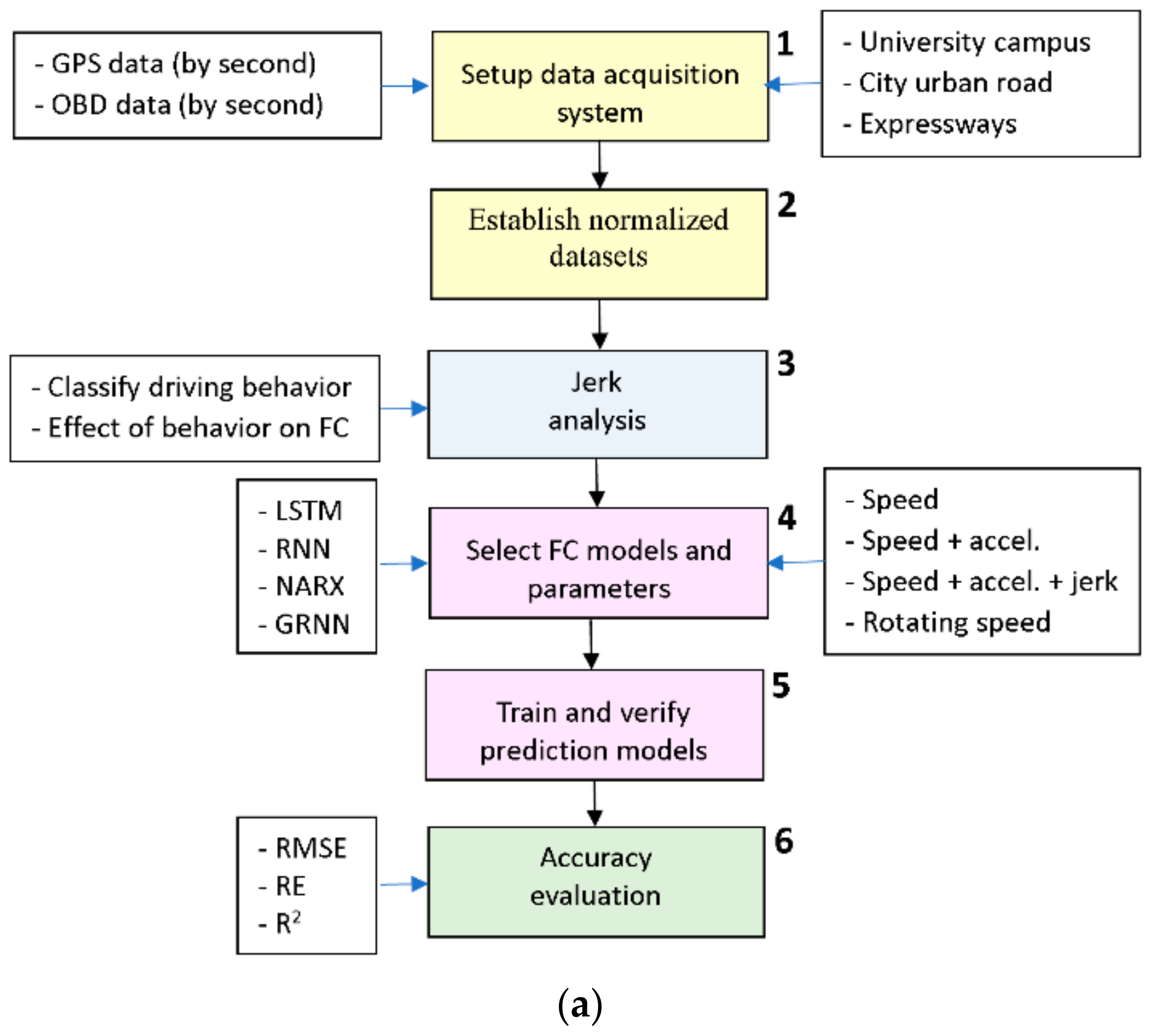
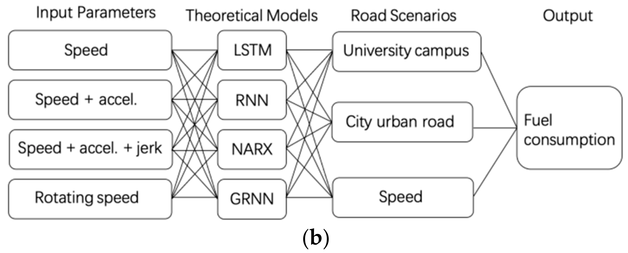
2. Research Framework

The overall framework of this study is shown in Figure 1a, and involves the following tasks:
Task 1: Establish a data acquisition system, and obtain the raw data (e.g., speed, rotating speed, and fuel consumption) for three road scenarios.
Task 2: Establish normalized datasets (speed, acceleration, jerk, rotating speed, and fuel consumption) using preprocessing data tools, such as derivation and normalization.
Task 3: Classify driving behaviors based on the jerk, and analyze the effects of various driving behaviors on the fuel consumption.
Task 4: Select four typical neural network models (LSTM, RNN, NARX, and GRNN), and four parameter combinations (speed, speed–acceleration, speed–acceleration–jerk, and rotating speed), which are shown in Figure 1b.
Task 5: Train and verify the fuel consumption prediction models in turn. Each neural network model input contains test training sets under three driving scenarios: the low-speed campus scenario; low– and medium–speed city scenario; and expressway driving scenario with low, medium, and high speeds.
Task 6: Evaluate the jerk’s effect on the accuracy of the fuel consumption prediction models, using RMSE, RE, and R2.

3. Data Description and Preprocessing

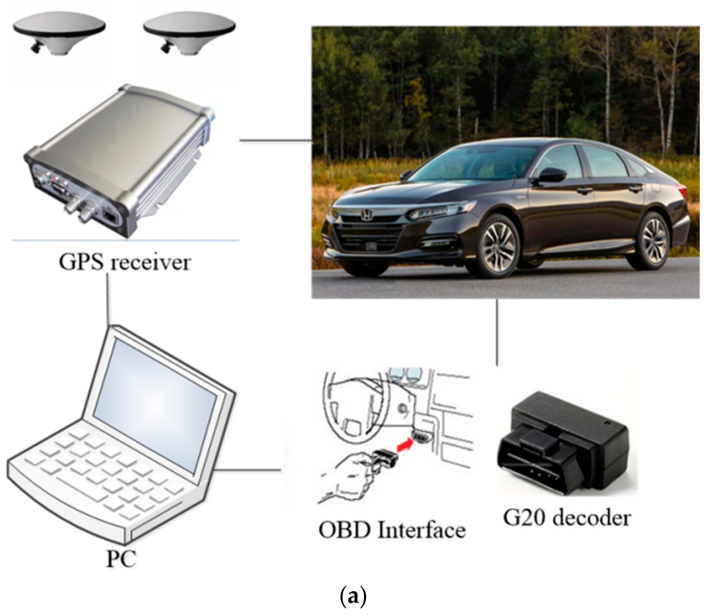
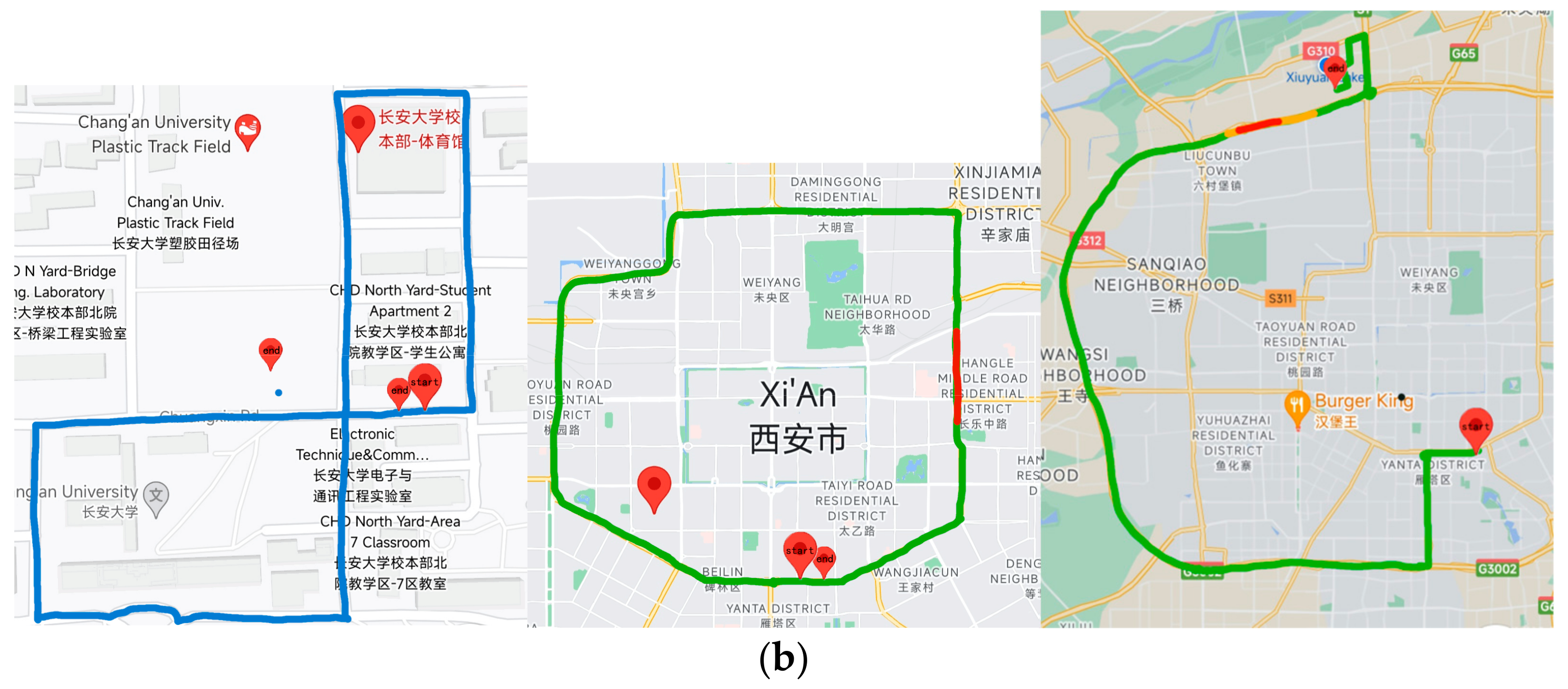
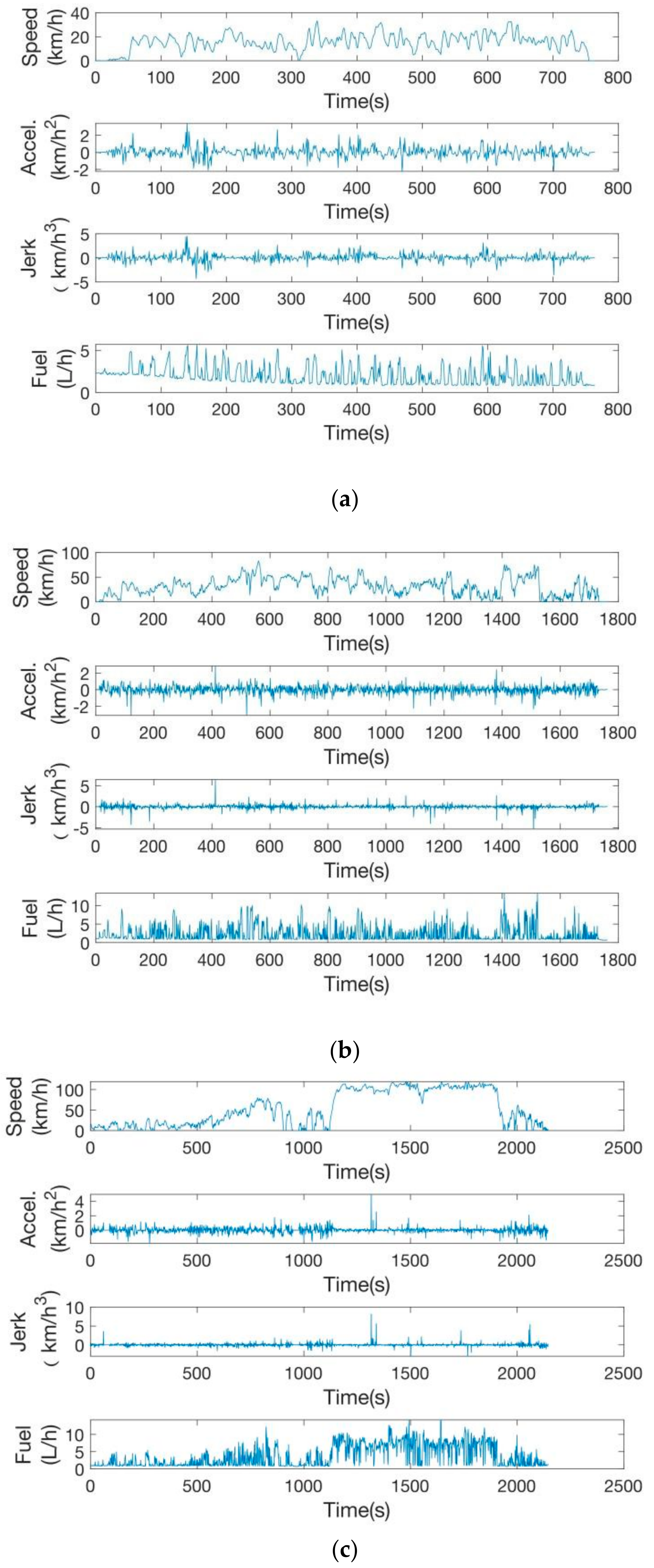
3.1. Data Description
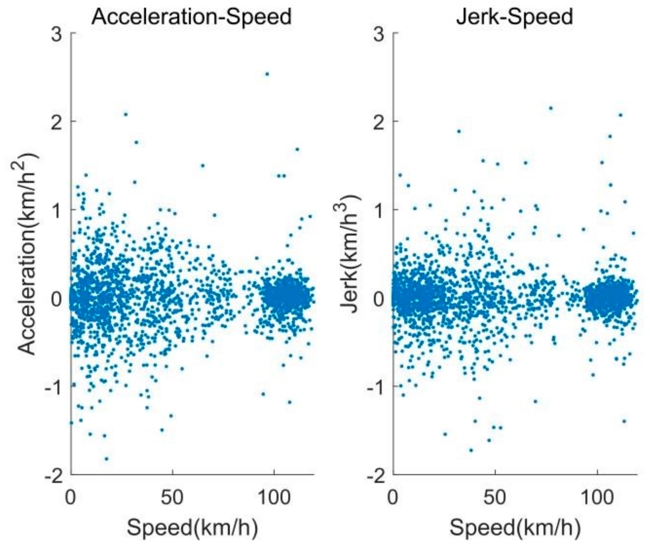
The experimental road conditions used in this study included low speeds on university campuses (0–40 km/h); low and medium speeds on urban roads (0–70 km/h); and all speeds on expressways with low, medium, and high speeds (0–120 km/h). On-board diagnostics (OBDs) and a global positioning system (GPS) were used to collect data under every working condition, and the data were accurate to two decimal places. The dataset included 13 vehicle driving parameters: latitude and longitude, speed, acceleration, jerk, and instantaneous fuel consumption. The dataset samples are shown in Table 1. The data in the third and sixth columns were obtained via GPS, and the data in the seventh and tenth columns were obtained via OBDs. The data acquisition platform and GPS tracks are shown in Figure 2a and Figure 2b, respectively.

3.2. Data Analysis

The dynamic changes in driving parameters under the low, medium, and high road scenarios are shown in Figure 3a–c, and an analysis of the statistical characteristics of the driving parameters is shown in Table 2. The characterization values of acceleration and jerk are derived through subtracting the speed and acceleration values before and after a one-second interval.
Ahn et al. [24] fitted a linear regression curve, and concluded that the higher the speed, the smaller the acceleration. This is because a vehicle engine must do more work to maintain the same acceleration at higher speeds, to overcome the increased air resistance. Therefore, the vehicle’s ability to accelerate or decelerate naturally decreases at higher speeds. The distribution maps of acceleration and jerk with speed are provided, to verify the rationality of the dataset in this study, as shown in Figure 4. As noted, both the acceleration and jerk decreased gradually with an increase in speed, so the dataset is reasonable, at least to some extent.

3.3. Data Preprocessing

Due to the different dimensionalities and dimensionality units of the parameters investigated, as well as the relatively larger variance in the speed, compared to those of other features in several orders of magnitude, speed occupies a dominant position in the learning algorithm, leading to an excessive speed weight in algorithm learning, and affecting the data analysis results. To address this issue, data standardization was used in this study for preprocessing, to eliminate the dimensionality impact between the data indicators, and ensure their comparability.
Min–max normalization, also known as deviation standardization, was used to linearly transform the raw data, achieving values within [−1, 1]. The conversion function is shown in Equation (1).
f x = 2 x M i n / M a x M i n 1
where M i n and M a x are the minimum and maximum values of the sample data, respectively.
Some data samples, before and after normalization, are shown in Table 3. As noted, after the raw data were subjected to data standardization, all parameters remained within [−1, 1]. Here, all indicators have the same order of magnitude, and are suitable for a comprehensive comparative evaluation. As the variances in the new data are normalized, the dimensionalities of each dimension are equivalent. Each dimension conforms to a normal distribution, with a mean of 0 and a variance of 1. This distribution helps prevent the speed range from being too large, and the training time from being too long, due to the initialization falling in a specific direction, and thereby avoiding an enormous impact on the fuel consumption prediction caused by the selection of different dimensionalities. After normalization, the identification of the optimal solution was expedited, and the accuracy of the models was improved.

4. Classification of Driving Behaviors Based on Jerk and Its Effects on Fuel Consumption

4.1. Introduction of Jerk

According to Newton’s second law and conservation of energy, the vehicle jerk is the rate of change of the resultant force exerted on the vehicle, and the vehicle’s power ultimately comes from fuel combustion work, so jerk is related to energy consumption.
In physics, jerk refers to the speed at which the acceleration of an object changes with time, and is usually represented by the symbol j , with units in m/s3. As a vector, the jerk can be expressed as the first derivative of acceleration, the second derivative of speed, or the third derivative of displacement, as Equation (2).
j t = d a t d t = d 2 v t d t 2 = d 3 r t d t 3
where a is acceleration, v is speed, r is displacement, and t is time. As noted, jerk represents the abrupt movement of vehicles. The jerk profile shows changes in the acceleration and deceleration rates, unlike the acceleration profile, which shows an increase or decrease in speed. The jerk profile indicates the driver’s abrupt changes during the driving operation.

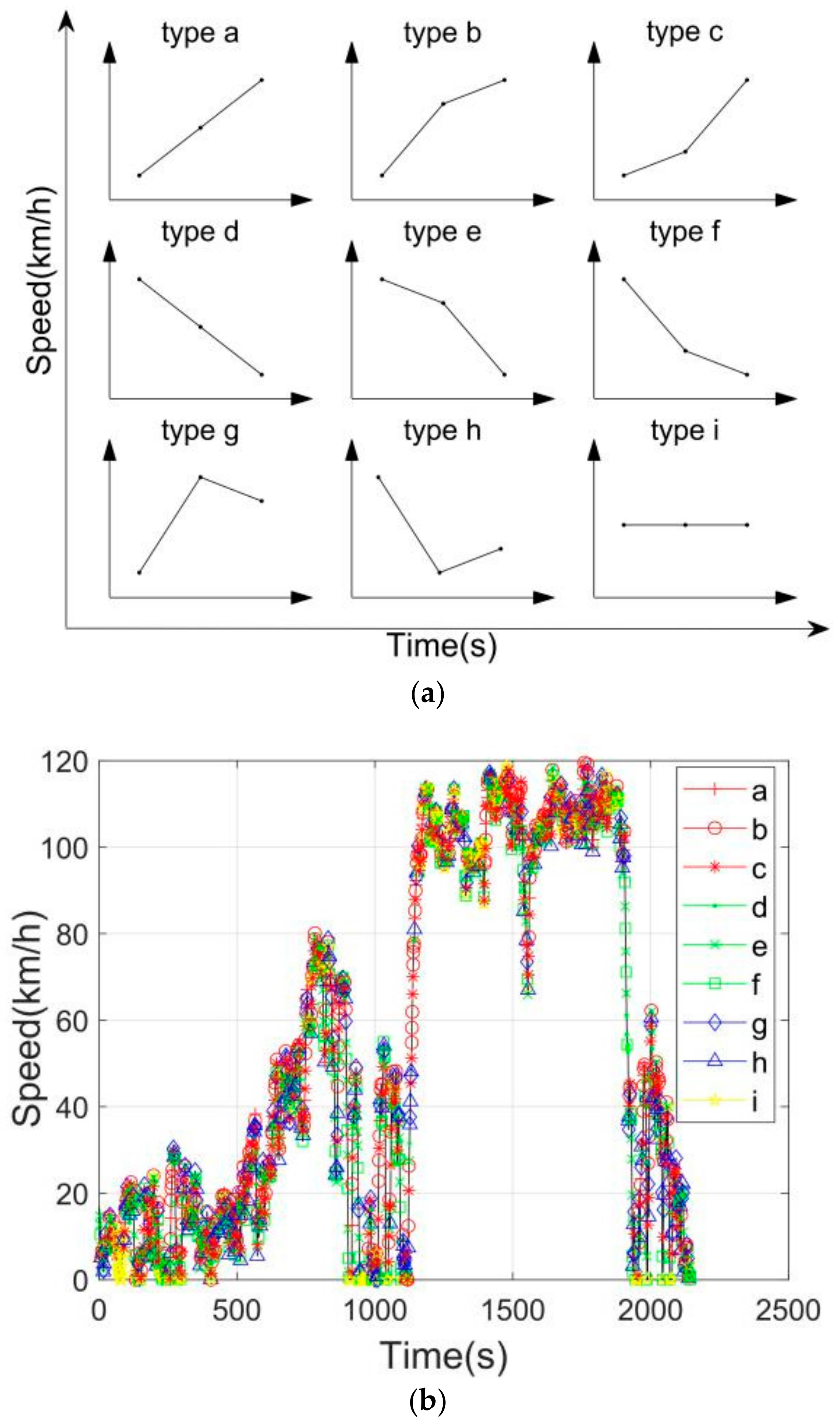
4.2. Driving Behavior Classification Based on Jerk

Equation (2) shows that the jerk, as the second derivative of speed, has a strong characterization effect on the fluctuation degree of the speed–time curve. In addition, the fluctuation degree of the speed–time curve significantly affects fuel consumption. Figure 5a classifies the jerk into nine types (a to i). Considering the speed–time curve of an expressway as an example, Figure 5b presents various jerk types in the speed–time curve, with different line types, according to the classifications outlined in Figure 5a.

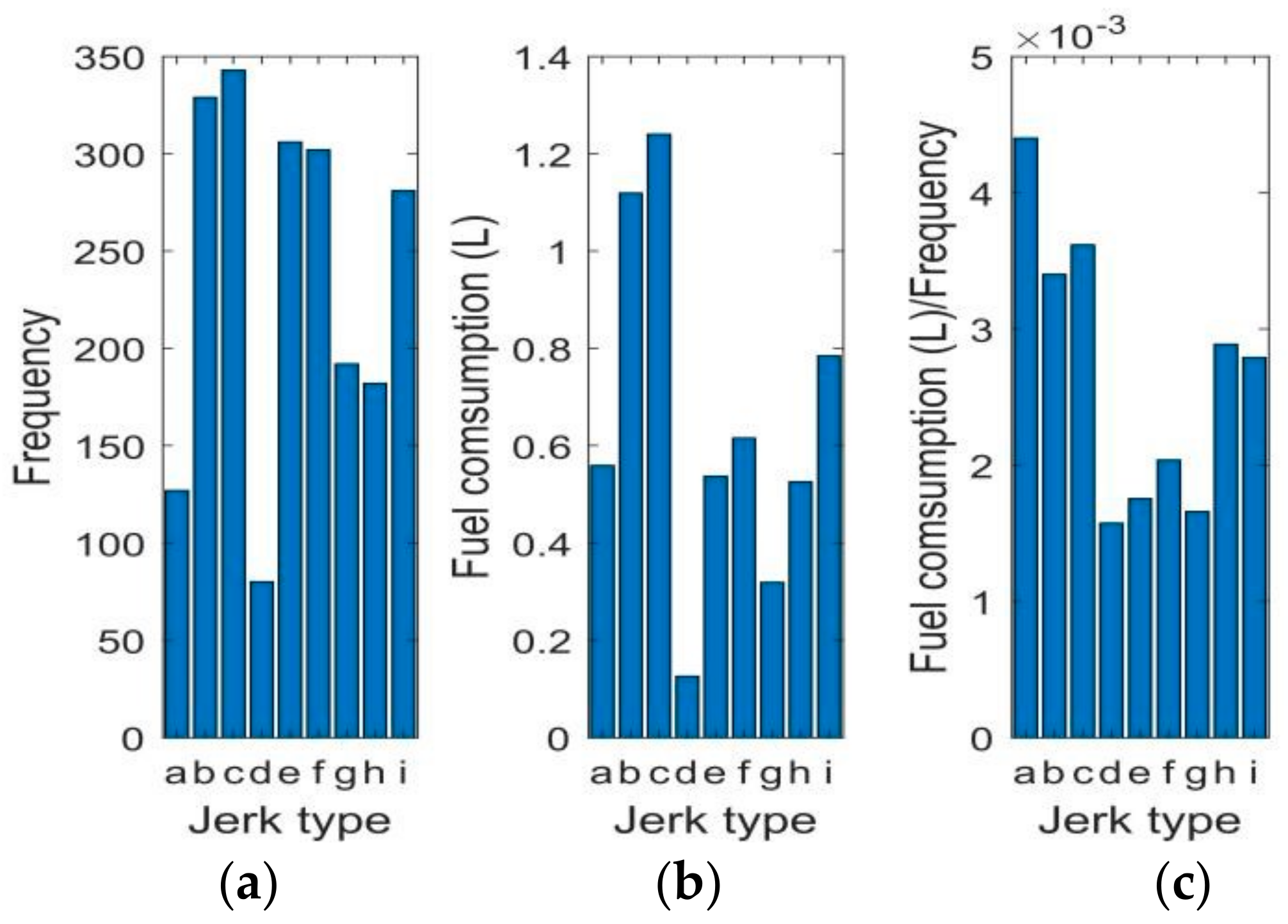
4.3. Effect of Jerk on Fuel Consumption

The occurrence frequency of various types of jerk, and the corresponding fuel consumption in the expressway scenario, were counted, and a histogram was plotted. Figure 6a–c show the effect of the jerk on the fuel consumption. As noted, the occurrence frequencies of different jerk types were different, and the corresponding fuel consumption of each type was also different. Thus, the jerk not only reflects driving behavior, but is also an essential factor affecting fuel consumption. Hence, it is of great significance to introduce jerk into neural networks as one of the inputs.
The speed, acceleration, and jerk are the main manifestations of driving behavior closely associated with fuel consumption, and the acceleration is the speed’s first derivative, and the jerk is the acceleration’s derivative. Therefore, these three variables depend on each other, and using any one of them will impact the prediction results. The following sections describe, in detail, the effects of different combinations on the prediction results.

5. Experimental Modelling

5.1. Modelling

The input and output variables of the neural network models are described in Table 4. This study selected four neural network models: LSTM, RNN, NARX, and GRNN. This experiment sought to study the effects on fuel consumption prediction under different neural network models, after introducing the jerk. Therefore, parameters such as the speed, acceleration, jerk, and rotating speed were selected for the experiment, and combined as the model inputs, and the fuel consumption was set as the output parameter. The parameter setting of each neural network model is provided in Table 5.

5.2. Model Calibration and Verification

Four input combinations were selected (speed, speed–acceleration, speed–acceleration–jerk, and rotating speed) to determine the parameters of the best input combination. Under the three road scenarios, the fuel consumption prediction performance of each group of the four neural network models, LSTM, RNN, NARX, and GRNN, was quantitatively analyzed. Therefore, it was necessary to carry out 4 × 4 × 3 = 48 groups of experiments. In each experimental group, 70% of the datasets were used for training, 15% for verifying the accuracy of the models, and 15% for testing. The calibration and verification of each model under the input condition combination of speed–acceleration–jerk are shown in Figure 7a–d.

6. Analysis of Experimental Results

6.1. Evaluation Indices

Three indices were selected to evaluate the fuel consumption prediction results, as Equations (3)–(5).
R M S E = 1 N t = 1 N y r e a l t y p r e t 2
R E = 1 N t = 1 N y r e a l t y p r e t y r e a l t
R 2 = 1 t = 1 N y r e a l t y p r e t 2 t = 1 N y r e a l t y ¯ 2
where N is the sample size, y p r e t is the predicted value, y r e a l t is the actual value, and y ¯ is the average value. When the RMSE and RE are small, and the R2 is closer to 1, the data fitting is better, which indicates that the independent variables offer a higher degree of explanation for the dependent variables.

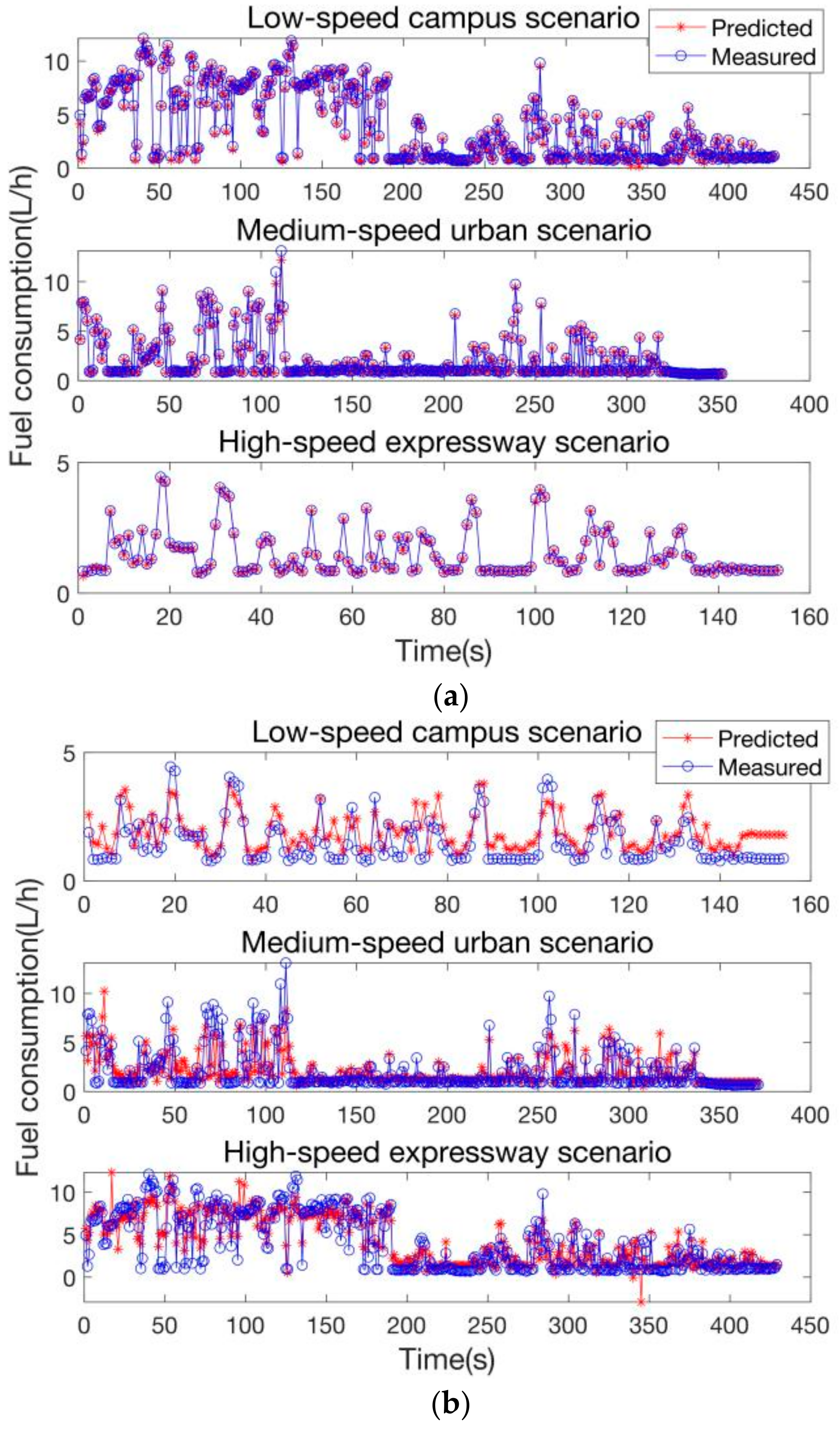
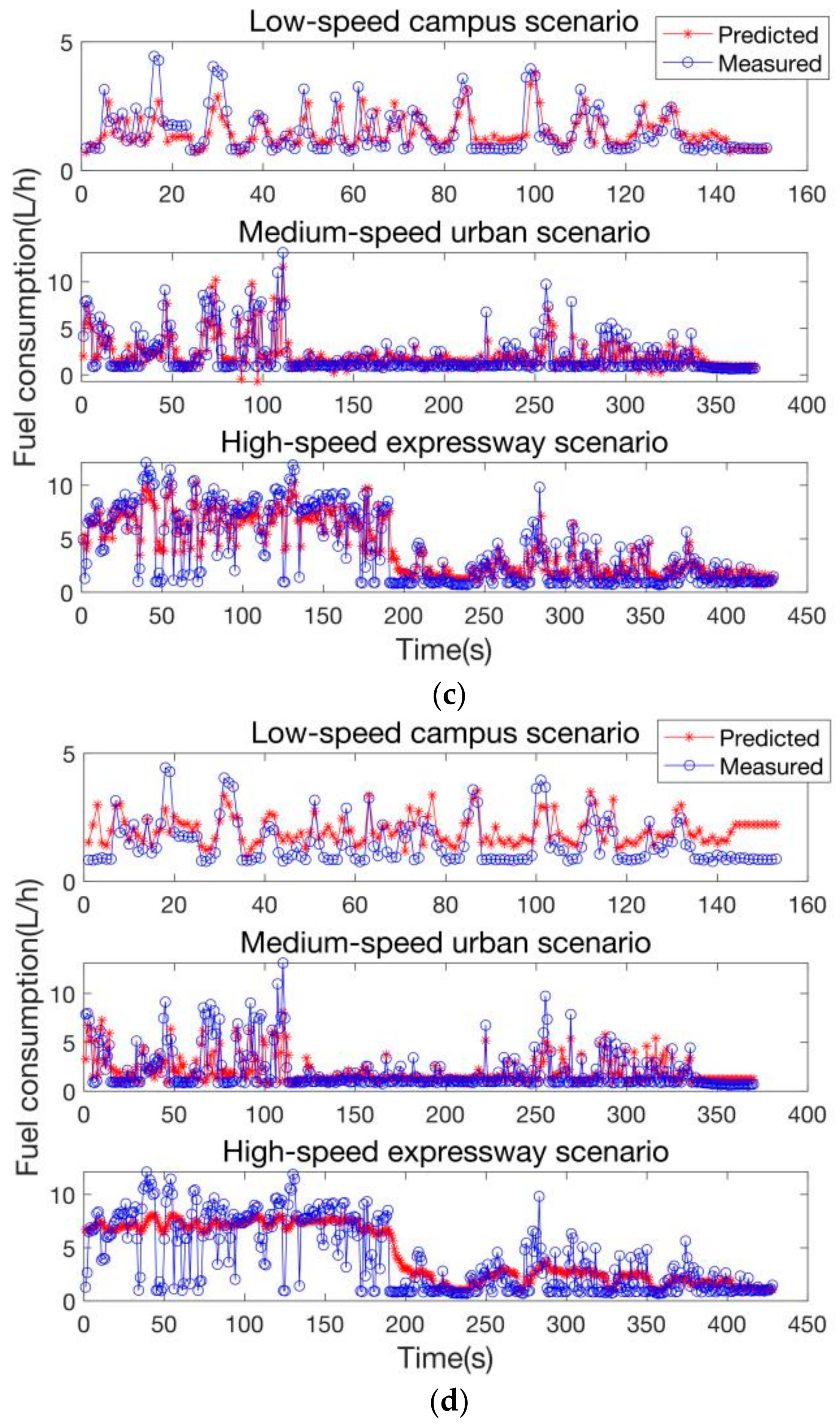
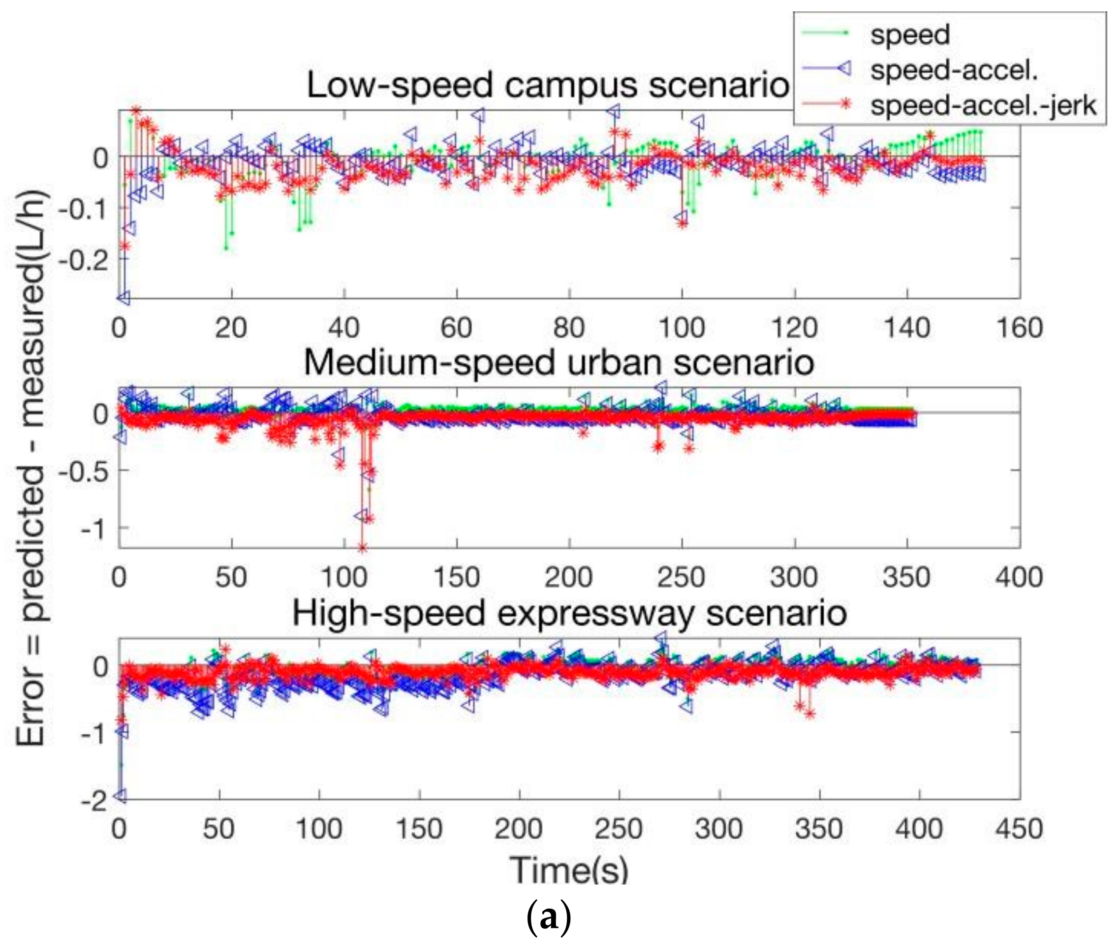
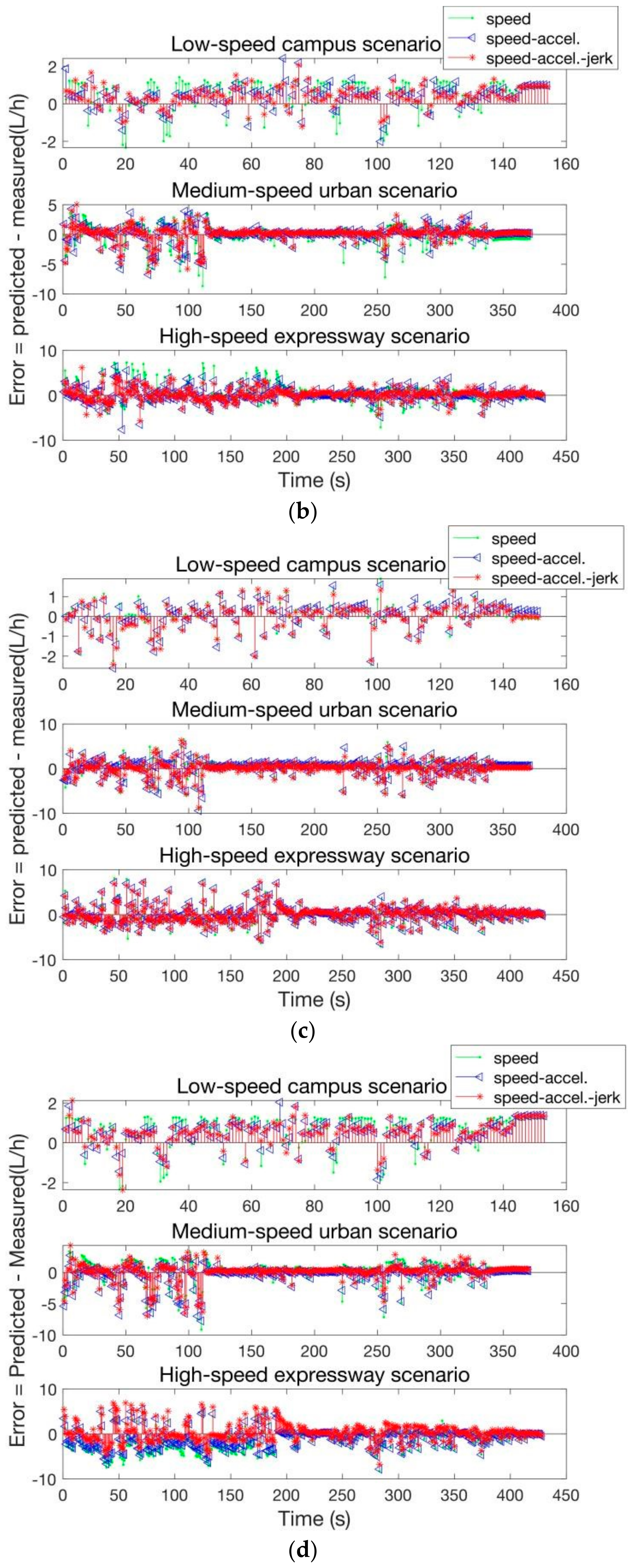
6.2. Experimental Analysis of Each Neural Network Model under Different Input Conditions

According to the analysis in Section 4.2, the jerk should be introduced into the input sequence of the neural network models as a factor. Figure 8a–d graphically show the absolute error diagrams of different input combinations (speed, speed–acceleration, speed–acceleration–jerk) for each neural network under three working conditions (campus, urban road, and expressway). As noted, when the speed, acceleration, and jerk are simultaneously used as the input characteristic variables, the prediction errors of each neural network are the smallest.
To further analyze the performance of different input variables for the four fuel consumption prediction models using a neural network under different road scenarios, the evaluation indices in Section 6.1 were calculated, as shown in Table 6. As noted, the prediction performance of each fuel consumption prediction model under different road scenarios gradually improved when speed, speed–acceleration, and speed–acceleration–jerk were selected as the training input combinations. The bold data in the Table 6 show the data results of the best performing model.
The prediction performance improvements in the four neural network models after considering the jerk are shown in Table 7 as percentages. As noted, for a low speed, medium speed, and high speed, each neural network offered the best fuel consumption prediction effects with the speed–acceleration–jerk as the combination input. The bold data in the Table 7 indicate the maximum and minimum values of the corresponding indicators. Here, the prediction results of each model improved after introducing jerk as an input, with the RMSE decreasing by up to 40.9% (LSTM, urban scenario), the RE decreasing by up to 68.2% (LSTM, urban scenario), and the R2 increasing by up to 41.8% (NARX, urban scenario).
Specifically, under the high-speed expressway scenario, LSTM achieved the most remarkable improvement, with the RMSE decreasing by 14.3%, the RE decreasing by 28.3%, and the R2 increasing by 9.7%. Under the low-speed campus scenario, NARX achieved the most remarkable improvement, with the RMSE decreasing by 34.3%, the RE decreasing by 43.0%, and the R2 increasing by 22.9%. Under the medium-speed urban scenario, LSTM achieved the greatest improvement in the RMSE and RE, with the RMSE decreasing by 40.9%, and the RE decreasing by 68.2%. NARX achieved the greatest improvement in the R2, with an increase of 41.8%.
Most of the large relative errors in prediction occurred in the following two cases: (1) when the vehicle came to a stop, the acceleration and the fuel consumption were not 0, and (2) a sudden acceleration or deceleration led to overly large relative prediction errors. The fuel consumption predictions of various neural networks could be properly trained, and the relative errors in fuel consumption prediction were also reduced when the jerk was introduced.

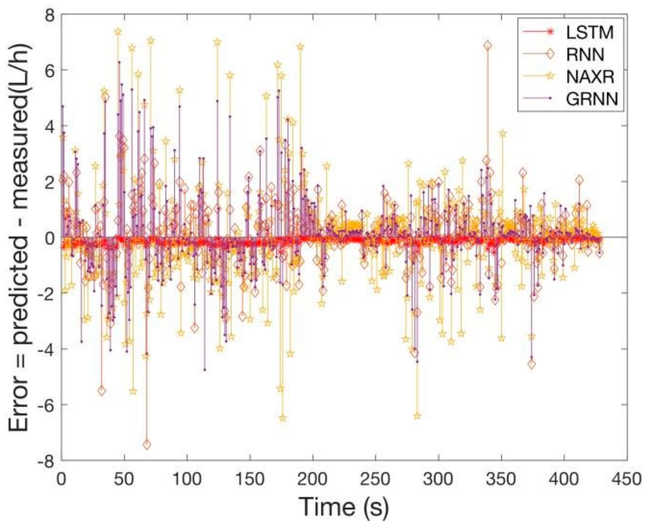
6.3. Comparison of FCP Models Using Neural Network

According to the above analysis, the prediction performance of each fuel consumption prediction model under different road scenarios gradually improved when the speed, speed–acceleration, and speed–acceleration–jerk were selected as input combinations. The effect of the jerk on the improvement of the fuel consumption prediction performance was deeply analyzed. This section reports a further quantitative analysis of the prediction results among the four neural network models. Among the LSTM, RNN, NARX, and GRNN neural network models, the prediction performance of the LSTM model outperformed the other three models under different input combinations (rotating speed, speed, speed–acceleration, speed–acceleration–jerk) and driving scenarios (low-speed campus scenario, medium-speed urban scenario, and high-speed expressway scenario). The RMSE and RE values of the LSTM model were the smallest (less than 0.1).
The RMSE values of the other three models were 11 to 17 times the value of LSTM in the low-speed campus scenario, 26 to 59 times the value of LSTM in the medium-speed urban scenario, and 15 to 33 times the value of LSTM in the high-speed expressway scenario. The RE of the other three models was 6 to 14 times the LSTM value in the low-speed campus scenario, 8 to 46 times the LSTM value in the medium-speed urban scenario, and 9 to 15 times the LSTM value in the high-speed expressway scenario. The R2 of LSTM was the largest, reaching about 0.99, while the values of the other three models were between 0.3 and 0.8. Notably, the rotating speed and fuel consumption were highly correlated, but the rotating speed was not always observable. Thus, the rotating speed was only used for performance comparisons in this study. Each performance index of the LSTM-based FCP model with the combination of speed–acceleration–jerk as the training input was equivalent to, or better than, the results when the rotating speed was the training input (Table 6).
Figure 9 graphically shows a comparison of the absolute prediction errors among the different models, considering jerk, for the expressway condition. As noted, all four models offered an excellent performance in predicting fuel consumption, but the LSTM neural network showed the best performance in all three evaluation indices.

7. Conclusions

This study involved the collection of datasets under three road scenarios to facilitate experimental analysis, with modelling of the long-term dependence characteristics of time series data via the selection of suitable neural network parameters. Furthermore, the effects of four combinations of input variables, under three road scenarios and four FCP models, were compared, to determine the accuracy of their fuel consumption prediction. Based on this study, the following conclusions can be drawn.
1. Among the LSTM, RNN, NARX, and GRNN neural network models, the prediction performance of the LSTM model was best under the different input combinations (rotating speed, speed, speed–acceleration, speed–acceleration–jerk) and different driving scenarios (low-speed campus scenario, medium-speed urban scenario, and high-speed expressway scenario). The RMSE value and RE value of the LSTM model were the smallest (less than 0.1). The RMSE values of the other three models were 11 to 17 times the RMSE of LSTM in the low-speed campus scenario, 26 to 59 times that of LSTM in the medium-speed urban scenario, and 15 to 33 times that of LSTM in the high-speed expressway scenario. The RE values of the other three models were 6 to 14 times the LSTM value in the low-speed campus scenario, 8 to 46 times the LSTM in the medium-speed urban scenario, and 9 to 15 times the LSTM in the high-speed expressway scenario. The R2 of LSTM was the largest, reaching about 0.99, while the values of the other three models were between 0.3 and 0.8.
2. After including the jerk as a new variable in the training input, all the neural network models improved in their fuel consumption accuracy. Notably, under the high-speed expressway scenario, LSTM achieved the most remarkable improvements, in which the RMSE decreased by 14.3%, the RE decreased by 28.3%, and the R2 increased by 9.7%. Under the low-speed campus scenario, NARX achieved the most remarkable improvement, in which the RMSE decreased by 34.3%, the RE decreased by 43.0%, and the R2 increased by 22.9%. Under the medium-speed urban scenario, LSTM achieved the greatest improvement in the RMSE and RE, with the RMSE decreasing by 40.9%, and the RE decreasing by 68.2%. Additionally, NARX achieved the greatest improvement in the R2, with an increase of 41.8%.

Author Contributions

Conceptualization, L.Z.; methodology, J.Y. and Z.X.; formal analysis, S.E.; validation, K.P.; writing—review and editing, Y.X.; writing—original draft, R.Y. All authors have read and agreed to the published version of the manuscript.

Funding

Financial support for this research was provided by the National Key Research and Development Program of China (Nos. 2021YFB2501200 and 2018YFB0105104); the 111 project (No. B14043), the Joint Laboratory of Internet of Vehicles of the Ministry of Education and China Mobile (No. 2012-364-812-105); the National Natural Science Foundation of China (No. 51278058); and the Fundamental Research Funds for the Central Universities, CHD (Nos. 300102240503 and 300102242502).

Data Availability Statement

The data used to support the findings of this study have not been made available because these data still need to be used in other unfinished studies.

Conflicts of Interest

The authors declare no conflict of interest.

References

  1. The State of the Global Climate; World Meteorological Organization: Washington, DC, USA, 2020.
  2. Fu, L.; He, K.; He, D.; Tang, Z.; Hao, J. A study on models of mobile source emission factors. Acta Sci. Circumstantiae 1997, 17, 474–479. (In Chinese) [Google Scholar]
  3. Ma, Y.; Lau, A.K.H.; Louie, P.K.K.; Li, T.; Luan, S. Application of vehicular emission models and comparison of their adaptability. Acta Sci. Nat. Univ. Pekin. 2008, 44, 308–316. [Google Scholar]
  4. California Air Resource Board. EMFAC User’s Guide; California Air Resource Board: Sacramento, CA, USA, 2020.
  5. Guo, H.; Zhang, Q.; Shi, Y.; Wang, D. Evaluation of the International Vehicle Emission (IVE) model with on-road remote sensing measurements. J. Environ. Sci. 2007, 19, 818–826. [Google Scholar] [CrossRef] [PubMed]
  6. Barth, M.; An, F.; Norbeck, J.; Ross, M. Modal emissions modelling: A physical approach. J. Transp. Res. Board 1996, 1520, 81–88. [Google Scholar] [CrossRef]
  7. An, F.; Barth, M.; Norbeck, J.; Ross, M. Development of comprehensive modal emissions model: Operating under hot-stabilized conditions. J. Transp. Res. Board 1997, 1587, 52–62. [Google Scholar] [CrossRef]
  8. Barth, M.; Younglove, T.; Wenzel, T.; Score, G.; An, F.; Ross, M.; Norbeck, J. Analysis of modal emissions from diverse in-use vehicle fleet. Transp. Res. Rec. J. Transp. Res. Board 1997, 1587, 73–84. [Google Scholar] [CrossRef]
  9. Jiménez-Palacios, L.J. Understanding and Quantifying Motor Vehicle Emissions with Vehicle Specific Power and TILDAS Remote Sensing; Massachusetts Institute of Technology: Cambridge, MA, USA, 1999. [Google Scholar]
  10. Rakha, H.; Ahn, K.; Trani, A. Development of VT-Micro model for estimating hot stabilized light duty vehicle and truck emissions. Transp. Res. Part D Transp. Environ. 2004, 9, 49–74. [Google Scholar] [CrossRef]
  11. Rahimi-Ajdadi, F.; Abbaspour-Gilandeh, Y. Artificial neural network and stepwise multiple range regression method for predicting fuel consumption of tractors. Measurement 2011, 44, 2104–2111. [Google Scholar] [CrossRef]
  12. Zhao, X.; Yao, Y.; Wu, Y.; Chen, C.; Rong, J. Research on combined prediction model of driving energy consumption based on principal component analysis and BP neural network. J. Transp. Syst. Eng. Inf. Technol. 2016, 16, 185–204. [Google Scholar]
  13. Wu, J.; Liu, J. Development of a predictive system for car fuel consumption using an artificial neural network. Expert Syst. Appl. 2011, 38, 4967–4971. [Google Scholar] [CrossRef]
  14. Topić, J.; Škugor, B.; Deur, J. Neural Network-Based Prediction of Vehicle Fuel Consumption Based on Driving Cycle Data. Sustainability 2022, 14, 744. [Google Scholar] [CrossRef]
  15. Li, Y.; Chen, M.; Zhao, W. Investigating long-term vehicle speed prediction based on BP-LSTM algorithms. IET Intell. Transp. Syst. 2019, 13, 1281–1290. [Google Scholar]
  16. Fitters, W.; Cuzzocrea, A.; Hassani, M. Enhancing LSTM prediction of vehicle traffic flow data via outlier correlations. In Proceedings of the 2021 IEEE 45th Annual Computers, Software, and Applications Conference (COMPSAC), Madrid, Spain, 12–16 July 2021; pp. 210–217. [Google Scholar]
  17. Zhu, W.; Wu, J.; Fu, T.; Wang, J.; Shangguan, Q. Dynamic prediction of traffic incident duration on urban expressways: A deep learning approach based on LSTM and MLP. J. Intell. Connect. Veh. 2021, 4, 80–91. [Google Scholar] [CrossRef]
  18. Hochreiter, S.; Schmidhuber, J. Long Short-Term Memory. Neural Comput. 1997, 9, 1735–1780. [Google Scholar] [CrossRef] [PubMed]
  19. Phan, H.; Andreotti, F.; Cooray, N.; Chén, O.Y.; De Vos, M. SeqSleepNet: End-to-end hierarchical recurrent neural network for sequence-to-sequence automatic sleep staging. IEEE Trans. Neural Syst. Rehabil. Eng. 2019, 27, 400–410. [Google Scholar] [CrossRef] [PubMed]
  20. Quan, R.; Zhu, L.; Wu, Y.; Yang, Y. Holistic LSTM for pedestrian trajectory prediction. I-EEE Trans. Image Process. 2021, 30, 3229–3239. [Google Scholar] [CrossRef] [PubMed]
  21. Doğan, E. Analysis of the relationship between LSTM network traffic flow prediction performance and statistical characteristics of standard and nonstandard data. J. Forecast. 2020, 39, 1213–1228. [Google Scholar] [CrossRef]
  22. Zhang, L.; Peng, K.; Zhao, X.; Asad, J. New fuel consumption model considering vehicular speed, acceleration, and jerk. J. Intell. Transp. Syst. 2023, 27, 174–186. [Google Scholar] [CrossRef]
  23. Xu, Z.; Wei, T.; Easa, S.; Zhao, X.; Qu, X. Modelling relationship between truck fuel consumption and driving behavior using data from internet of vehicles. Comput-Aided Civ. Infrastruct. Eng. 2018, 33, 209–219. [Google Scholar] [CrossRef]
  24. Ahn, K.; Rakha, H.; Trani, A.; Van Aerde, M. Estimating vehicle fuel consumption and emissions based on instantaneous speed and acceleration levels. J. Transp. Eng. 2002, 128, 182–190. [Google Scholar] [CrossRef]
Figure 1. Research framework: (a) the task flow; (b) the evaluated combinations of input parameters, theoretical models, and road scenarios.
Electronics 12 03638 g001aElectronics 12 03638 g001b
Figure 2. The data acquisition platform and global positioning system(GPS) tracks: (a) the data acquisition platform: a Honda car and equipment (global positioning system(GPS) and On-board diagnostics(OBDs)); (b) the campus, city, and expressway GPS tracks.
Electronics 12 03638 g002aElectronics 12 03638 g002b
Figure 3. Dynamic changes in the main parameters under the various road scenarios: (a) the main data for the low-speed campus scenario, (b) the main data for the low- and medium-speed urban scenario, (c) the all-speed data for the low-, medium-, and high-speed expressway scenario.
Electronics 12 03638 g003
Figure 4. Relationship of the acceleration and jerk with speed.
Electronics 12 03638 g004
Figure 5. Relationship of acceleration and jerk with speed. Classification of jerk: (a) schematic diagram of nine jerk types, and (b) expressway speed curves marked with different types of jerk.
Electronics 12 03638 g005
Figure 6. Relationship of acceleration and jerk with speed. Effect of the jerk type on fuel consumption: (a) frequency, (b) fuel consumption, and (c) fuel consumption per frequency.
Electronics 12 03638 g006
Figure 7. The model calibration and verification of each neural network model: (a) LSTM, (b) RNN, (c) NARX, (d) GRNN.
Electronics 12 03638 g007aElectronics 12 03638 g007b
Figure 8. Absolute prediction error diagrams of each neural network model: (a) LSTM, (b) RNN, (c) NARX, (d) GRNN.
Electronics 12 03638 g008aElectronics 12 03638 g008b
Figure 9. Comparison of the prediction results among the different models, considering jerk, under the expressway condition.
Electronics 12 03638 g009
Table 1. Sample datasets.
DateTimeLon 1 (°N)Lat 2 (°E)Alt 3 (km)Speed (km/h)RS 4 (r/min)Ins Fuel 5 (L/h)Cum Fuel 6 (L)Mileage (km)
16 January 2021 18:52:023413.91110,856.648377.895216.7636711190.92224.905581,677,555
16 January 202118:52:033413.91210,856.644379.102815.855189020.88224.905901,677,561
16 January 202118:52:043413.91210,856.641379.477414.739938590.94224.906121,677,565
16 January 202118:52:053413.91210,856.639379.528112.655658640.96224.906361,677,568
16 January 202118:52:063413.91210,856.637379.451010.483058750.93224.906681,677,572
16 January 202118:52:073413.91210,856.635379.29137.575238400.94224.906921,677,574
16 January 202118:52:083413.91210,856.633379.18856.209047490.93224.907241,677,577
1 Lon = longitude (°N), 2 Lat = latitude (°E), 3 Alt = altitude (km), 4 RS = rotating speed (r/min), 5 Ins Fuel = instantaneous fuel consumption (L/h), 6 Cum fuel = cumulative fuel consumption (L).
Table 2. Statistical characteristics of the main driving parameters under the different road scenarios.
InputCampusCityExpressway
V 1A 2J 3V 1A 2J 3V 1A 2J 3
Average15.480.040.6730.761.52 × 10−4−0.0153.260.010.01
Max33.283.414.4982.722.836.44119.494.948.14
Min0.01−2.22−4.290−3.10−5.310−1.82−2.99
Variance49.970.340.59311.600.200.241.80 × 1030.120.17
1 V = speed (km/h), 2 A = acceleration (km/h2), 3 J = jerk (km/h3).
Table 3. Data before and after normalization.
Raw DataNormalized Data
Speed (km/h)Acceleration (km/h2)Jerk (km/h3)Fuel (L)SpeedAccelerationJerkFuel
15.9000−0.10000.50000.88000.13380.25370.29630.0148
14.7000−0.2000−0.30000.94000.12370.23880.22220.0192
12.7000−0.6000−0.20000.96000.10690.17910.23150.0207
10.5000−0.20000.20000.93000.08840.23880.26850.0185
7.6000−0.7000−0.10000.94000.06400.16420.24070.0192
Table 4. Description of input and output variables.
VariableVariable Description
Input v t Vehicle speed
a t Vehicle acceleration speed
j t Vehicle jerk speed
y t Fuel consumption at time t
r(t)Rotating speed
Output y ^ t + 1 Fuel consumption at the next time step
Table 5. Parameter setting of each neural network model.
Neural NetworkInputNetwork LayerParameter SettingOutput
LSTMSpeed,
acceleration,
jerk,
rotating speed
Hidden neurons60 × 180 × 60Fuel consumption
Dropout layers0.2 × 0.3 × 0.2
RNNHidden neurons10
NARXHidden neurons10
Delays d2
GRNNHidden neuronsNumber of samples
Table 6. The prediction performance of different models under three road scenarios.
Parameter CombinationModelDriving Scenario
CampusCityExpressway
RMSERE R2RMSERE R2RMSERE R2
Rotating speedLSTM0.0300.0330.9980.0290.0180.9980.0900.0670.994
RNN0.4850.2190.7960.7480.2990.8221.3590.5480.779
NARX0.4850.2290.7951.7040.5350.7731.6700.6240.665
GRNN0.5210.2470.7650.8840.4250.8201.6790.6130.740
Speed–
acceleration–
jerk
LSTM0.0330.0170.9980.0260.0140.9980.0480.0330.996
RNN0.4660.2000.8111.2710.3740.6101.2420.3850.842
NARX0.3770.1530.8751.5100.6470.4511.6070.4890.736
GRNN0.5450.2340.7431.5280.5060.4631.5430.4830.781
Speed–
acceleration
LSTM0.0400.0240.9970.0440.0440.9910.0560.0460.991
RNN0.5120.2250.7711.4480.4570.5171.4500.4500.806
NARX0.5740.2670.7121.6880.6860.3181.8400.6400.688
GRNN0.6240.3300.6631.5810.5280.4241.7090.5200.731
SpeedLSTM0.0540.0470.9950.0550.0650.9880.0650.0510.988
RNN0.7320.3450.6741.9150.4940.4792.0700.7640.664
NARX0.7530.3010.5761.8270.7460.3071.9060.7130.609
GRNN0.6980.4230.5741.7240.6890.4051.9280.6380.694
Table 7. Analysis of the model prediction performance improvements after considering jerk.
Driving Scenario
CampusCityExpressway
RMSERE R2RMSERE R2RMSERE R2
LSTM−17.5%−29.2%+0.1%−40.9%−68.2%+0.7%−14.3%−28.3%+9.7%
RNN−8.9%−11.0%+5.2%−12.2%−18.0%+18.0%−14.3%−14.4%+4.5%
NARX−34.3%−43.0%+22.9%−10.5%−5.7%+41.8%−12.7%−23.6%+7.0%
GRNN−12.7%−29.0%+13.3%−3.4%−4.2%+9.2%−9.7%−7.1%+6.8%
Disclaimer/Publisher’s Note: The statements, opinions and data contained in all publications are solely those of the individual author(s) and contributor(s) and not of MDPI and/or the editor(s). MDPI and/or the editor(s) disclaim responsibility for any injury to people or property resulting from any ideas, methods, instructions or products referred to in the content.

