Article

Advancements in Household Load Forecasting: Deep Learning Model with Hyperparameter Optimization

by
Hamdi A. Al-Jamimi
1,2,*,
Galal M. BinMakhashen
1,2,
Muhammed Y. Worku
3,4 and
Mohamed A. Hassan
3,*
1
Computer Science and Engineering, King Fahd University of Petroleum and Minerals, Dhahran 31216, Saudi Arabia
2
Research Excellence, King Fahd University of Petroleum & Minerals, Dhahran 31261, Saudi Arabia
3
Interdisciplinary Research Center for Renewable Energy and Power Systems (IRC-REPS), Research Institute, King Fahd University of Petroleum and Minerals, Dhahran 31261, Saudi Arabia
4
Electrical Engineering Department, King Fahd University of Petroleum and Minerals, Dhahran 31261, Saudi Arabia
*
Authors to whom correspondence should be addressed.
Electronics 2023, 12(24), 4909; https://doi.org/10.3390/electronics12244909
Submission received: 14 October 2023 / Revised: 29 November 2023 / Accepted: 30 November 2023 / Published: 6 December 2023

Abstract

:
Accurate load forecasting is of utmost importance for modern power generation facilities to effectively meet the ever-changing electricity demand. Predicting electricity consumption is a complex task due to the numerous factors that influence energy usage. Consequently, electricity utilities and government agencies are constantly in search of advanced machine learning solutions to improve load forecasting. Recently, deep learning (DL) has gained prominence as a significant area of interest in prediction efforts. This paper introduces an innovative approach to electric load forecasting, leveraging advanced DL techniques and making significant contributions to the field of energy management. The hybrid predictive model has been specifically designed to enhance the accuracy of multivariate time series forecasting for electricity consumption within the energy sector. In our comparative analysis, we evaluated the performance of our proposed model against ML-based and state-of-the-art DL models, using a dataset obtained from the Distribution Network Station located in Tetouan City, Morocco. Notably, the proposed model surpassed its counterparts, demonstrating the lowest error in terms of the Root-Mean-Square Error (RMSE). This outcome underscores its superior predictive capability and underscores its potential to advance the accuracy of electricity consumption forecasting.

1. Introduction

Modern power generation facilities require a consistent and uninterrupted supply of electricity to effectively meet load demands [1]. This necessitates precise predictions of both current and future load requirements, minimizing errors. To achieve this, researchers and scientists have focused on developing an efficient method known as load forecasting [2,3]. This technique involves forecasting future electricity consumption demands and playing a vital role in decision-making processes like unit commitment, network management, dispatch strategies, fuel allocation, and other operational aspects [4,5,6]. The increasing integration of renewable energy resources (RES) into the energy mix and the transformation of the traditional electric grid into a more intelligent, flexible, and interactive system have elevated the importance of electrical load forecasting in smart grid planning and operation [7,8,9,10,11]. The multi-stage real-time stochastic operation of grid-tied multi-energy microgrids (MEMGs) via the hybrid model predictive control (MPC) and approximate dynamic programming (ADP) approach was studied [10]. Accurate multi-node load forecasting is the key to the safe, reliable, and economical operation of the power system [11]. Since power generated from RES fluctuates based on factors such as weather conditions like irradiation and wind speed, maintaining a careful balance between power demand and supply through accurate load forecasting becomes crucial [10,11,12,13].
Electric load consumption data are a time series that comprise a sequence of observations at regular time intervals, encompassing both linear and nonlinear components [9]. Overestimating load requirements can result in excess power generation and market trading, while underestimation can lead to a mismatch between demand and supply, causing grid instability. Predicting electric load is a challenging task due to its high volatility and uncertainty, whether in the distribution system or within individual households [14,15]. Load forecasting (LF) serves as a methodology for predicting future load demands by analyzing historical data and identifying dependency patterns within its time-step observations. Its applications in power system operation and planning are extensive, encompassing demand response, scheduling, unit commitment, energy trading, system planning, and energy policy [14]. Precise LF is essential for power companies and decision makers to strike a balance between supply and demand, prevent power interruptions due to load shedding, and avoid an excess reserve of power generation [14]. Accurate forecasting enables utilities to plan demand response management, unit commitment, load dispatch, contingency planning, and optimal load flow with minimal resource wastage and cost overruns. The complexity, uncertainty, and the multitude of factors influencing predictions make LF a challenging task, categorized as a type of time-series problem necessitating specialized solutions [15]. Depending on the time horizon, forecasting can be short-term (hours to a week), medium-term (a week to a year), or long-term (over a year) [8]. Forecasting outputs can be pointing forecasts, providing a single estimated value of the future load, or density forecasts, offering estimates of the future load probability distribution, either pointwise or interval-wise. Various techniques are employed based on the forecast horizon. Although there is not a universally agreed-upon classification determined by the predictive horizon, it is crucial to acknowledge that diverse forecasting scenarios come with distinct challenges and advantages, requiring varied modeling strategies [9,10,16].
Currently, the prevailing approach involves utilizing classical and deep machine learning algorithms, genetic algorithms, wavelet analysis, singular spectral analysis, and similar methodologies [2]. Nevertheless, the selection of methods is contingent upon the specific problem under consideration and the inherent structure of the initial data. Recent studies have extensively reviewed state-of-the-art techniques in LF [17,18,19,20,21,22,23,24,25,26], categorizing them into two main groups: statistical and machine learning (ML) methods. Statistical methods, including autoregressive integrated moving average (ARIMA), linear regression, and exponential smoothing, map input data to output. These methods function by adhering to pre-established rules and assumptions, crafting a prediction model that delineates the relationship between variables [27]. It entails fitting project-specific probabilities to historical data and generating load predictions through statistical inference. These techniques are frequently characterized by their speed, simplicity, interpretability, and computational efficiency. However, they suffer from uncertainty and low accuracy, particularly in high nonlinear systems. ML techniques, such as artificial neural networks (ANN), deep learning (DL), and recurrent neural networks, have more complex setups and longer training times but offer higher accuracy and performance. As a branch of AI, the methodology of ML empowers computers to learn and adjust automatically through experience [28,29]. The process includes training a model on a dataset and employing the trained model to predict outcomes on new data. While these techniques can capture intricate relationships and patterns, they demand meticulous feature selection and parameter tuning [29]. DL represents an advanced iteration of ML, utilizing layered algorithms and neural networks with multiple hidden layers to acquire knowledge and formulate predictions [28,29]. DL architectures usually comprise intricately layered networks with multiple hidden layers, enabling them to grasp intricate data representations and generate precise predictions, especially when handling extensive and intricate datasets. However, it is important to note that they can be computationally demanding and necessitate substantial amounts of data for effective training [28,29].
This paper introduces a novel approach to electric LF, employing advanced DL techniques. The key contributions of this study are as follows: Firstly, the presentation of a hybrid predictive model that integrates DL methods to enhance the accuracy of multivariate-to-multivariate time series forecasting in the energy domain. Secondly, the use of a Keras Regressor wrapper and Randomized Search cross-validation (CV) technique to optimize the DL model’s hyperparameters, improving its overall performance. Additionally, an innovative early stopping algorithm is developed to efficiently monitor and terminate the training process, conserving computational resources. The research also delves into feature significance and provides a comprehensive analysis of how varying the number of features influences training performance, shedding light on feature selection’s impact. Through extensive simulations and experiments, the proposed model consistently outperforms existing approaches, demonstrating the lowest Root-Mean-Square Error (RMSE) in comparisons. Lastly, the study encompasses a thorough literature review of recent deep-learning models used for power consumption prediction, offering insights into the field’s advancements and trends.
The aspects of novelty of this work can be summarized as follows:
  • Hybrid predictive model—this paper introduces a novel hybrid predictive model that integrates DL methods for electric LF. While DL is a well-explored area, the unique contribution lies in the hybrid nature of our model, combining different DL techniques to enhance the accuracy of multivariate time series forecasting in the energy domain. The specific combination and integration of these techniques represent a novel approach.
  • Hyperparameter optimization and early stopping algorithm—we employ a Keras Regressor wrapper and Randomized Search cross-validation technique for hyperparameter optimization, enhancing the overall performance of the DL model. Additionally, we introduce an innovative early-stopping algorithm designed to efficiently monitor and terminate the training process, conserving computational resources. These elements contribute to the novelty of our proposed methodology for training DL models in the context of electric LF.
  • Comparative analysis and superior predictive capability—the comparative analysis evaluates the performance of our proposed model against other state-of-the-art DL models, using a real-world dataset from the Distribution Network Station in Tetouan City, Morocco. Our proposed model consistently outperforms existing approaches, achieving the lowest RMSE. This outcome underscores its superior predictive capability, representing a significant advancement in accuracy compared to the current state of the art.
The remainder of this paper is structured as follows: Section 2 summarizes the related work. Section 3 provides an in-depth examination of the dataset, conducts relevant data analysis, and introduces both DL and ML models. In Section 4, we delve into the details of our proposed hybrid model. Section 5 is dedicated to presenting the results of our experiments, including comprehensive comparisons between our model and previous approaches. Finally, Section 6 serves as the conclusion of this paper, summarizing key findings and outlining potential future research directions.

2. Related Work

Anticipating electricity consumption holds a pivotal role in the effective management and strategic planning of the energy usage. The electric load profile in metropolitan areas exhibits complex cyclic and seasonal patterns influenced by industrial production, weather, and human activities. Contemporary research in this field is focused on exploring aspects such as smart grid technologies, the integration of renewable energy sources, and the establishment of local energy communities [30]. Numerous LF methods have been developed over the years, categorized into statistical models and modern ML and artificial intelligence (AI) models [10]. Statistical models include linear models like autoregressive (AR), moving average (MA), autoregressive moving average (ARMA), and ARIMA, seasonal ARIMA (SARIMA), as well as Kalman filtering algorithms, grey models, and exponential smoothing [11]. These models assume stationary and linear time series data following known statistical distributions [8]. They effectively capture the historical trends and seasonality inherent in consumption data [31,32]. However, they may struggle with big data and nonlinear relationships between load values and external factors. Modern techniques based on ML and AI offer an alternative to statistical models by autonomously extracting patterns and trends from data [5]. Commonly used ML models for time series forecasting include support vector regression (SVR), and ANNs [4,5,31].
DL approaches, such as recurrent neural networks (RNN), gated recurrent networks, and (LSTM), have also gained attention for their ability to model complex non-linear patterns [10,32,33]. DL methods have been applied to LF with promising results. DL, a specialized domain within the broader field of ML, harnesses the power of ANNs with multiple layers to comprehend and represent intricate mappings between input and output data [34,35]. The momentum behind DL surged notably with the introduction of Multi-Layer Perceptrons (MLP) and the refinement of back-propagation algorithms during the 1980s and 1990s [35]. One of the distinguishing features of DL techniques is their effective handling of the vanishing gradient problem, setting them apart from shallower models. Consequently, models based on DL exhibit superior capabilities in dealing with complex functions, achieving higher accuracy in their predictions [36]. The perspective on DL has gained substantial traction, especially in recent times, driven by the unprecedented availability of extensive datasets and the advancement of sophisticated algorithms [34,36]. DL methods employ multi-layer network models to construct linear or non-linear functions that aim to minimize the correlation between input data and output response. This evolution is such that the ML techniques discussed in preceding sections have undergone a transformative process, evolving into DL models through the incorporation of additional mapping layers. In the specific context of LF, DL approaches necessitate the construction of intricate networks, offering distinct advantages over classical techniques, particularly in multi-point scenarios within the load profile. However, it is crucial to acknowledge certain drawbacks, notably in terms of computational complexity and limitations in deterministic point forecasting [37]. Despite these challenges, the appeal of DL approaches for LF remains strong due to their remarkable ability to capture short- and long-term dependencies within input data. Moreover, DL models provide viable solutions to computational challenges, making them more preferable than shallower learning models. A review of DL methods applied to LF revealed that DL-based approaches are more accurate and stable than traditional statistical techniques and time series analysis [16]. DL models such as Long Short-Term Memory (LSTM) are effective in electric LF [38,39]. Therefore, DL would be an important candidate among other methods for electric-LF.
The recent surge in ML and DL models has brought forth sophisticated tools capable of unraveling complex patterns and dependencies in electricity consumption. The advanced ML and DL models showcased excellence in handling non-linear relationships and long-term dependencies, making them particularly suitable for precise energy forecasting within building contexts [40]. The hybrid models, amalgamating multiple forecasting techniques, present a promising avenue by leveraging the unique strengths of different algorithms to enhance the accuracy of predictions [41,42]. The effectiveness of ML and DL models crucially relies on feature engineering techniques. These techniques involve extracting relevant information from data to ensure that the models can discern and capture the key factors influencing electricity consumption. The application of such techniques not only facilitates improved energy management decisions but also contributes to grid stability and supports the integration of distributed generation [43,44]. The continuous evolution and progress in this field contribute to the generation of precise and timely forecasts, thereby aiding in effective energy planning and optimization. In a specific study [45], a novel approach is proposed, utilizing generative adversarial networks (GAN) to generate parallel energy consumption data. These generated data are then combined with the original dataset to enhance the performance of energy consumption prediction. The evaluation of the proposed method involves metrics such as the mean absolute error (MAE), mean absolute percentage error (MAPE), and Pearson correlation coefficient. Another study [22] puts forth a method that integrates convolutional neural network (CNN) and long short-term memory (LSTM) for the prediction of electric charges. The performance of this approach is compared with other models, including LSTM, XGBoost, and radial basis functional network (RBFN), using metrics such as RMSE, MAPE, MAE, and goodness of fit (R2). Taking a different approach [46], a non-parametric regression model is introduced, utilizing Gaussian process (GP) for the selection of input data to predict electricity consumption in buildings. The study evaluates the effectiveness of support vector regression (SVR), LSTM, and random forest (RF) through metrics such as symmetric mean absolute percentage error (sMAPE), MAE, and RMSE. Various models and metrics have conducted extensive analyses to predict energy consumption [47,48,49,50]. These studies involve evaluating the performance of models like random forest (RF), support vector regression (SVR), multilayer perceptron (MLP), and others. The metrics employed in these evaluations include the mean absolute percentage error (MAPE), R2, RMSE, and more. A comprehensive summary of the most recent related work is presented in Table 1.
On the one hand, predicting short-term load is challenging due to its high correlation with residents’ stochastic behavior, which makes it difficult to predict [20]. On the other hand, short- and very short-term loading predictions favor ML methods that are capable of modeling building and occupancy characteristics, as well as environmental data. In this study, we aim to study the performance of ML modeling using a hybrid technique that integrates DL methods to enhance electricity LF.

3. Materials and Methods

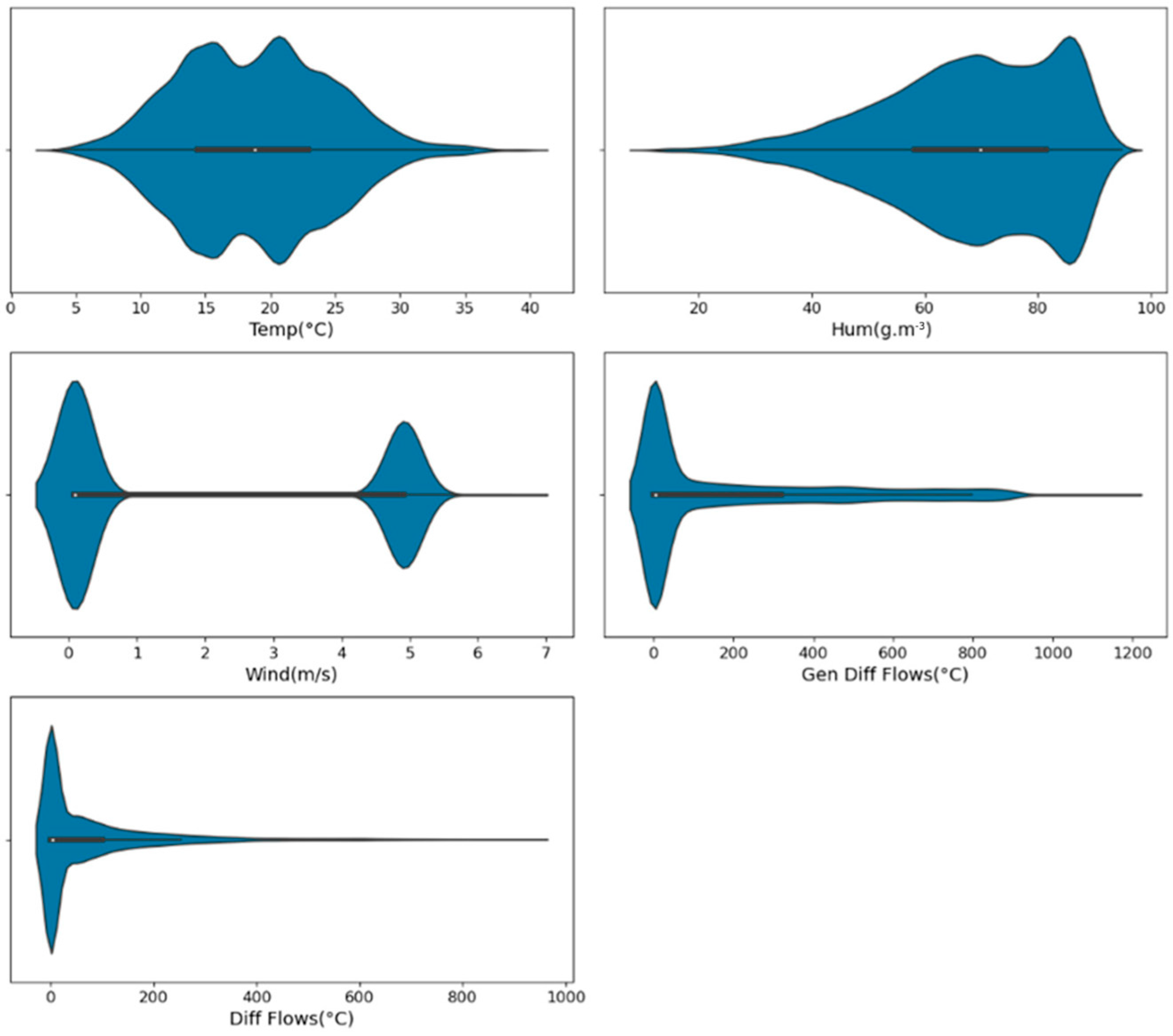
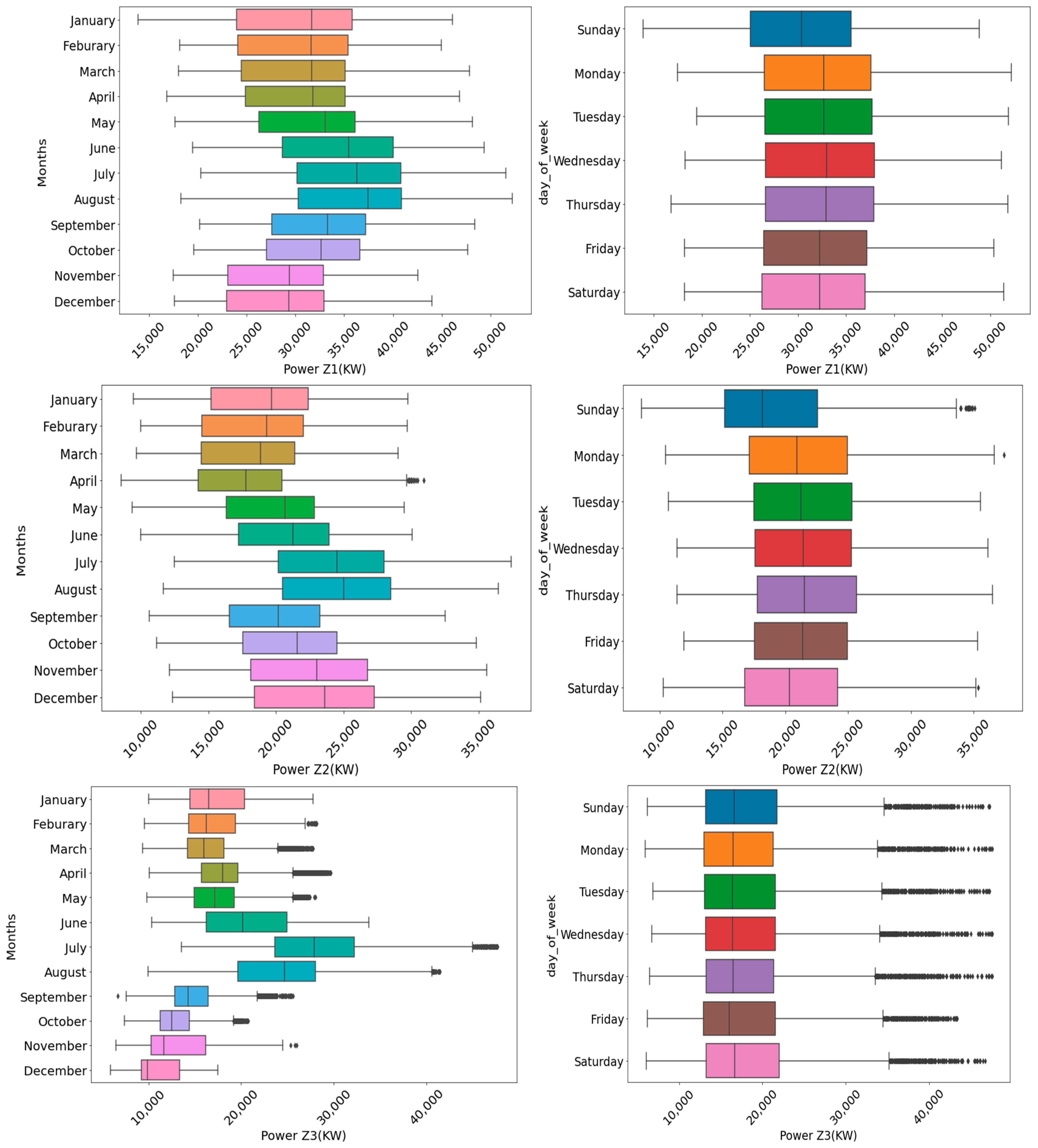
3.1. Dataset Description

The Tetouan power consumption dataset, publicly available and used in this study, spans a one-year time series from 1 January 2017, to 31 December 2017. The dataset captured power consumption measurements at regular 10 min intervals, ensuring a complete and continuous set of data without any missing values. The dataset was collected from three different distribution substations located in the Quads, Boussafou, and Smir zones of Tetouan City, situated in northern Morocco. In addition to power consumption readings, the dataset includes various weather-related information such as temperature and humidity. These weather data provide additional context for analyzing and understanding the relationship between power consumption and environmental conditions. Each data entry in the dataset provides power consumption information at 10 min intervals. Additionally, complementary data about the calendar and weather conditions are included, enhancing the dataset’s richness and potential for deeper analysis. By leveraging the comprehensive Tetouan power consumption dataset, researchers can gain insights into the dynamics of power consumption in different districts of the city. This dataset, with its detailed power consumption measurements, calendar information, and weather conditions, offers valuable opportunities to study load patterns, forecast power demands, and develop advanced prediction models for short-term LF.
This paper conducts a statistical analysis of the dataset to explore the relationships among the different variables, as shown in Table 2. The statistical analysis conducted on the dataset involves computing various descriptive statistics for each variable. The rationale behind this analysis is to gain insights into the distribution, central tendency, variability, skewness, and kurtosis of the data. By calculating these statistics for each variable in the dataset, we can gain a better understanding of the data’s characteristics. These statistics can help identify patterns, outliers, and the overall shape of the distributions. They provide a summary of the dataset’s properties and serve as a foundation for further analysis and decision making.
Figure 1 depicts the distribution of each data factor namely the temperature, humidity, wind speed, general diffusion flows, and diffusion flows. As observed from Table 2 both the general diffusion flows and diffusion flows are suffering a positive tail, Figure 1 shows how severely the diffusion flows are skewed. The wind factor has two clear modes, while the temperature factor has two close modes.
Figure 2 illustrates the power consumption of the three zones by looking at the month and day of a week. For Zone 1 and 2, the power consumption is at its peak in August, while Zone 3 July is the month of power’s highest demand. Also, the month boxplot of Zone 3 showed many outliers with high power consumption in February, March, April, May, July, August, September, October, and November. Such abnormal power consumption is also reflected in the Day boxplot subfigure. In general, the power consumption during the weekdays is almost similar. However, in Zone 1 and 2, the power consumption is a little less during Sundays.
Pearson’s correlation coefficient, denoted as RHO, measures the strength and direction of linear relationships between two variables. It ranges from −1 (perfect negative correlation) to +1 (perfect positive correlation), with 0 indicating no linear relationship. When applied to evaluate relationships between independent and dependent variables, RHO helps identify which independent variables are more strongly associated with the dependent variables in a linear manner. The analysis conducted in our study is illustrated in Figure 3. The Temperature variable exhibited the highest correlation when compared to other independent variables, with correlation coefficient values of 0.44, 0.39, and 0.49 in relation to the three target variables (Power Consumption_Zone1, Power Consumption_Zone2, and Power Consumption_Zone3). On the other hand, the Humidity variable showed comparable correlation coefficient values to the three targets, ranging from −0.23 to −0.29, suggesting a moderate negative linear relationship. In contrast, the Wind Speed and General Diffuse Flows variables demonstrated low correlation coefficient values, with the Diffuse Flows variable exhibiting nearly no correlation with the three target variables. These findings provide valuable insights into which independent variables have the most substantial linear impact on the dependent variables, aiding in model selection and interpretation.

3.2. Machine Learning Methods

3.2.1. Linear Regression

Linear regression models the relationship between an output variable and one or more input variables. It is one of the most widely used techniques for data analysis and prediction. For the case of one input variable, we assume that the output variable is a linear function of that input variable. The equation of the simple linear regression model is
y = β 0 + β 1 x + ϵ
where y is the dependent variable, x is the independent variable, β 0 is the intercept, β 1 is the slope, and ϵ is the error term.
The simple linear regression is scaled up to model the relationship between a set of multiple input variables to one output variable. In this case, we assume that the output variable is a linear combination of the input variables. The equation of the multiple linear regression model is
y = β 0 + β 1 x 1 + β 2 x 2 + + β k x k + ϵ
The goal of linear regression is to estimate the values of the parameters ( β 0 , β 1 , , β k ) that best fit the data. There are different methods to perform this, such as ordinary least squares, maximum likelihood, or Bayesian inference.

3.2.2. Ridge Regression

Ridge regression enhances the linear regression by slightly changing its cost function, which results in less overfit models. It does so by adding a penalty term to the ordinary least squares (OLS) estimator, which shrinks the coefficients of the model to zero. This penalty term is proportional to the square of the L2-norm of the coefficients, also known as the ridge parameter. By choosing an appropriate value for the ridge parameter, we can trade off some bias for lower variance and improve the prediction accuracy of the model. The Ridge regression minimizes the following cost function:
J ( ϕ ) = i = 0 n ( ( k = 0 p   β k x k ) y i ) 2 + λ j p β j 2
where y is the actual output, λ is coefficient that controls the Ridge penalty applied to the regression model. Often Ridge regression is employed in scenarios where the input variables are highly correlated. Figure 3 shows Temp and Hum input variables with 0.5 or more correlation with other input variables.

3.2.3. Support Vector Regression

Support vector regression (SVR) is an ML technique that can be used to model the relationship between a dependent variable and one or more independent variables. SVR is based on the idea of finding a function that has at most epsilon deviation from the actual data points for all the data points and at the same time is as flat as possible 1. In other words, SVR tries to fit a smooth curve that minimizes the error between the predicted and observed values, while also avoiding overfitting the data.
SVR has some advantages over other regression methods, such as being able to handle nonlinear and high-dimensional data, being robust to outliers and noise, and having a unique solution that does not depend on the initial conditions. However, SVR also has some drawbacks, such as being computationally expensive, requiring careful tuning of the parameters, and being sensitive to the scale of the input features.

3.3. Deep Learning Methods

Deep Forwarded Neural Network (DFNN)

DFNN represents a classical model in DL research, revered for its ability to sift through extensive input variables and deliver highly accurate predictions in regression tasks [99]. Its architectural design is structured into three pivotal components: the input layer, the hidden layer, and the output layer. To ward off overfitting during training, a dropout layer is strategically inserted between the input and hidden layers, selectively pruning neurons at random intervals to enhance generalization performance [100]. DFNN’s training process encompasses fine-tuning the hidden layers, neuron configurations, and the number of iterations. Rigorous cross-validation procedures are employed to scrutinize the model’s performance, rigorously assessing its efficacy across test and training datasets.

4. Proposed Approach

Predicting electricity power consumption is crucial for enhancing the efficiency and productivity of utility systems. ML models are renowned for their accuracy in this context. The goal of our study is to predict the electricity power consumption every 10 min, and/or every hour with the determining objective of which approach is the most successful. The proposed methodology combines data preprocessing, DL model building, learning rate schedule, early stopping, and model evaluation techniques to train a DL model for regression tasks on the provided dataset, as shown in Figure 4.
While our hybrid predictive model has been meticulously designed to enhance multivariate time series forecasting accuracy within the energy sector, its adaptability extends to other domains such as industry, residential, and commercial applications. The model’s flexibility allows for customization to address the unique characteristics of each sector, leveraging techniques like forward DL, hyperparameter optimization, and feature significance analysis. Beyond the energy sector, the model’s potential lies in optimizing operational efficiency, from production schedules in industries to demand-side management in residential areas and strategic energy planning for commercial establishments. Real-world applications and case studies in diverse settings can underscore the model’s broader impact, showcasing its versatility in contributing to accurate forecasting across various sectors. While acknowledging the need to consider sector-specific factors in the adaptation process, our work suggests that the methodologies employed hold promise for advancing forecasting capabilities beyond the energy sector, offering a valuable tool for enhancing operational planning and resource allocation across different industries.

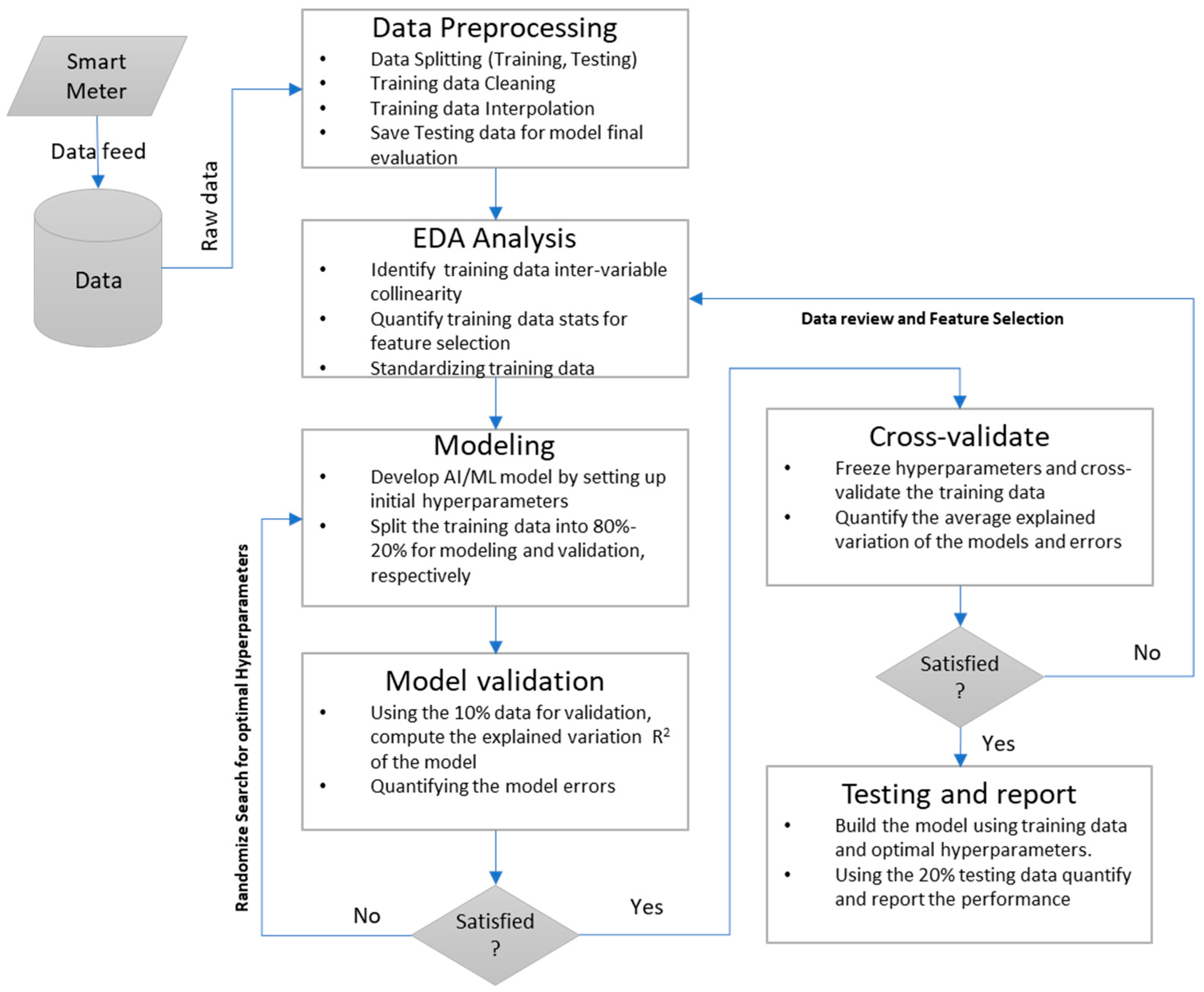
4.1. Data Preprocessing

In the data preprocessing stage, several techniques are employed to transform the input variable “DateTime” into more appropriate forms, including Year, Month, Day, Hour, and Minute. Moreover, the time scale is adjusted from 10 min intervals to 60 min intervals to enable short-term load forecasting for the subsequent hour. Additionally, standardization is applied to the input variables as part of the data preprocessing pipeline.

4.2. Model Development

Model development comprises different components, as summarized in the following subsections.

4.2.1. Deep Learning

In this study, a DL model was constructed using the Keras library [101,102], particularly the Sequential model, which facilitates the creation of a linear stack of layers. The model architecture comprises densely connected layers, known as Dense layers, which incorporate activation functions to introduce non-linearity and dropout regularization to prevent overfitting. The model was compiled using the mean squared error (MSE) loss function, which measures the discrepancy between predicted and actual values, and the RMSprop optimizer, which adjusts the model’s parameters to minimize the loss function during training [103].

4.2.2. Learning Rate Scheduling

The ReduceLROnPlateau callback from the Keras library was employed in this study to implement the learning rate scheduling [104,105]. This technique dynamically adjusts the learning rate during the training process based on the validation loss. By monitoring the validation loss, the callback reduces the learning rate when the loss plateaus, aiming to enhance the model’s convergence and overall performance. This adaptive adjustment of the learning rate facilitates efficient training by allowing the model to make smaller steps toward the optimal solution when progress becomes slower.

4.2.3. Early Stopping

The EarlyStopping callback from the Keras library was employed in this study to implement the early stopping technique [106]. During the training process, this callback continuously monitors the validation loss and halts the training if the loss does not improve for a predefined number of epochs. This technique helps prevent overfitting by stopping the model from further optimizing its performance on the training data at the expense of generalization. By selecting the model with the best performance on the validation set, early stopping allows for the retention of the model that exhibits optimal performance without compromising its ability to generalize to unseen data.

4.3. Model Training and Evaluation

To evaluate the efficacy of our proposed model, we partitioned the dataset into training and testing subsets, adhering to an 80–20 ratio. Subsequently, we conducted a comparative analysis by juxtaposing the predicted power consumption values against the corresponding ground truth data within identical time intervals. This rigorous assessment facilitated the evaluation of the model’s accuracy and overall performance. The DL model is trained using the fit function, which iterates over the specified number of epochs. During training, mini-batches of size 64 are utilized, allowing for efficient processing of the training data [107]. The learning rate scheduling and early stopping callbacks are incorporated into the training process, ensuring dynamic adjustment of the learning rate, and stopping the training if the validation loss does not improve. This approach optimizes the model’s convergence and prevents overfitting, leading to improved performance and generalization capabilities. Following the training phase, the trained model is employed to make predictions on the preprocessed testing set. The predictions obtained are then evaluated using commonly used regression evaluation metrics described in the next subsection. By examining these evaluation metrics, the performance and effectiveness of the trained model can be assessed.

4.4. Hyperparameter Optimization

To optimize the hyperparameters of the Keras model, we employed a combination of techniques. First, we utilized Randomized Search CV, which is a randomized search algorithm from scikit-learn, to perform a hyperparameter search. The search space included various hyperparameters such as the learning rate, dropout rate, number of epochs, batch size, and activation function. This allowed us to explore a range of hyperparameter combinations and identify the best configuration based on the specified evaluation metric, which was the negative mean squared error. To integrate the Keras model with the hyperparameter search, we used the Keras Regressor wrapper. This wrapper provided a scikit-learn compatible interface for the Keras model, enabling us to incorporate it into the Randomized Search CV process. The Keras Regressor wrapper allowed us to create and compile the Keras model within the create_model function, which defined the model architecture and optimization parameters based on the given hyperparameters. After performing the hyperparameter search and obtaining the best hyperparameters, we trained the Keras model with these optimal settings. The model was trained on preprocessed training data, using the best number of epochs and batch size determined by Randomized Search CV. The training process involved fitting the model to the training data and updating the model’s weights and biases iteratively to minimize the mean squared error loss. Finally, we evaluated the performance of the trained model by making predictions on the preprocessed test set. The predicted values were compared with the actual target values using different evaluation metrics. These metrics provided insights into the accuracy and predictive capability of the best Keras model identified through the hyperparameter optimization process. By combining Randomized Search CV, the Keras Regressor wrapper, model training with the best hyperparameters, and model evaluation, we were able to efficiently search for and assess the performance of the optimal Keras model for the given dataset.

5. Results and Discussion

In this section, we present the comprehensive results of our study on household LF, showcasing the efficacy of our proposed hybrid DL model with hyperparameter optimization. We begin by examining the model’s performance in predicting electricity consumption at both 10 min intervals and hourly intervals, shedding light on its capabilities in capturing intricate temporal patterns. Furthermore, we delve into a rigorous evaluation of the model’s accuracy, utilizing a range of statistical metrics to quantify its forecasting precision. These results not only highlight the advancements achieved in household LF but also underline the potential for enhancing energy management systems with state-of-the-art predictive models. To assess the efficacy of our ML models, we employ five distinct statistical metrics that have been previously identified as valuable for power consumption forecasting. These metrics are defined as follows:
R2 assesses the proportion of variance in the target variable that is explained by the model. It ranges from 0 to 1, with higher values indicating a better fit.
R 2 = 1 S S r e s S S t o t
where S S r e s is the sum of squared residuals (sum of squared differences between the actual and predicted values), and S S t o t is the total sum of squares (the sum of squared differences between the actual values and the mean of the actual values).
RMSE represents the standard deviation of the residuals and is expressed in the same units as the target variable.
R M S E = 1 n i = 1 n ( y i y ^ i ) 2
where n is the number of samples; y i and y ^ i are the actual and predicted values of the target variable for the i t h sample, respectively.

5.1. Machine Learning Methods

We assessed some baseline ML methods to analyze the input variables’ relationship with the target variable and establish the baseline performance of traditional ML methods using the Tetouan City dataset. Table 3 presents the configuration of machine learning methods.
We built ML models and assessed them to establish a baseline performance using the Tetouan City dataset. Table 4 tabulates the performance of three known machine learning techniques. We noticed that coefficients of determination R2 were low in all experiments. This affects the RMSE per model and indicates the need for better models.

5.2. Deep Neural Network Design

In this experiment, we employ DL methods by constructing a neural network model, defining its architecture, training it with data, and evaluating its performance using appropriate metrics. The algorithm to build the DNN was stated by creating a sequential model using ‘Sequential ()’ from ‘tensorflow.keras.models’, which allows for building a neural network model by stacking multiple layers sequentially. The dense layers were added to the model to ensure full connection among the neurons in the consecutive layers. The model uses a rectified linear unit (relu) as an activation function. We applied regularization to the model’s weights in the dense layers. In this experiment, L1 regularization with a regularization strength of 0.001 was used. Additionally, dropout regularization was utilized to avoid overfitting by randomly setting a fraction of input units to 0 during training to reduce the co-adaptation of neurons. The model was compiled with the loss function set to MSE metric to calculate the mean squared difference between the predicted and actual values. The RMSprop optimizer was incorporated as an adaptive learning rate optimization algorithm that helps in faster convergence. Lastly, Callbacks are used for dynamic adjustment of the learning rate and early stopping.
The main structure and number of parameters to learn per layer are summarized in Table 5. To avoid overfitting, the DNN was designed with dropout layers where the algorithm drops 20% of the computed information randomly to regularize the model. Moreover, the design uses the relu activation function due to it being able to be computed faster than other complex activation functions.
In this model, ‘ReduceLROnPlateau’ reduces the learning rate when a metric (in this case, validation loss) stops improving [31]. ‘EarlyStopping’ stops training when the metric (validation loss) does not improve for a certain number of epochs. Table 6 demonstrates the obtained performance measurements in the context of the three targets. In addition, it displays the RMSE associated with predicting the power load at its peak point.
Figure 5, Figure 6 and Figure 7 present distinct figures, each encapsulating the outcomes derived from our proposed DL model in the context of Power Consumption prediction for three distinct zones, as specified within our dataset. These figures collectively provide an intricate analysis of our DL model’s predictive capabilities, offering valuable insights into its performance across different zones and sample sizes. Each figure consists of three subfigures: (top) comprehensively illustrates the results encompassing all testing samples, offering a holistic view of the model’s performance over time, (middle) selectively focuses on a subset, specifically 10% of the testing samples, enabling a more detailed examination of predicted and actual data points, and (bottom) narrows the scope further, emphasizing only 1% of the testing samples. This deliberate reduction in sample size enhances the visual clarity of the plots, facilitating a meticulous assessment of the alignment between predicted and actual data points.

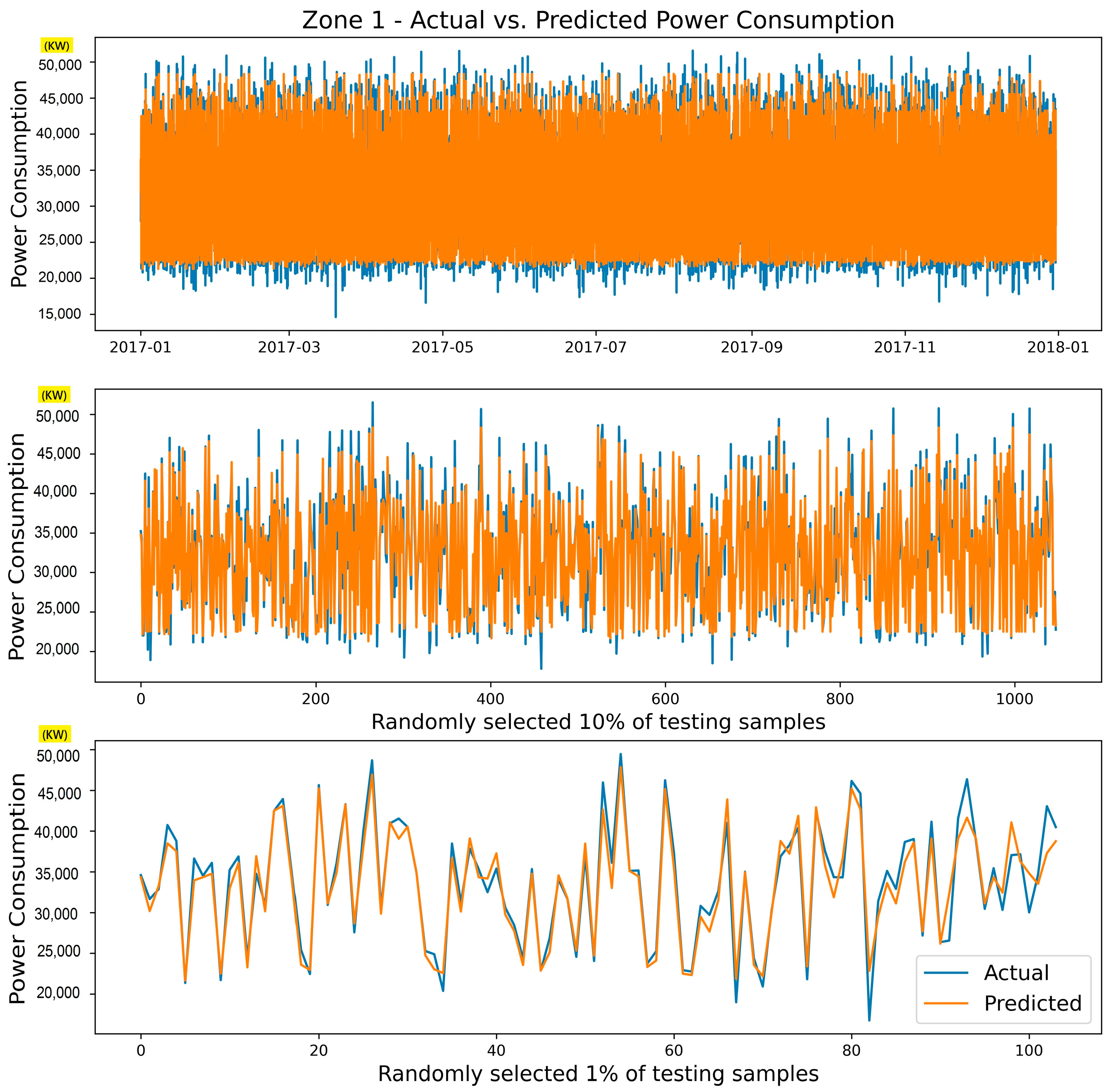
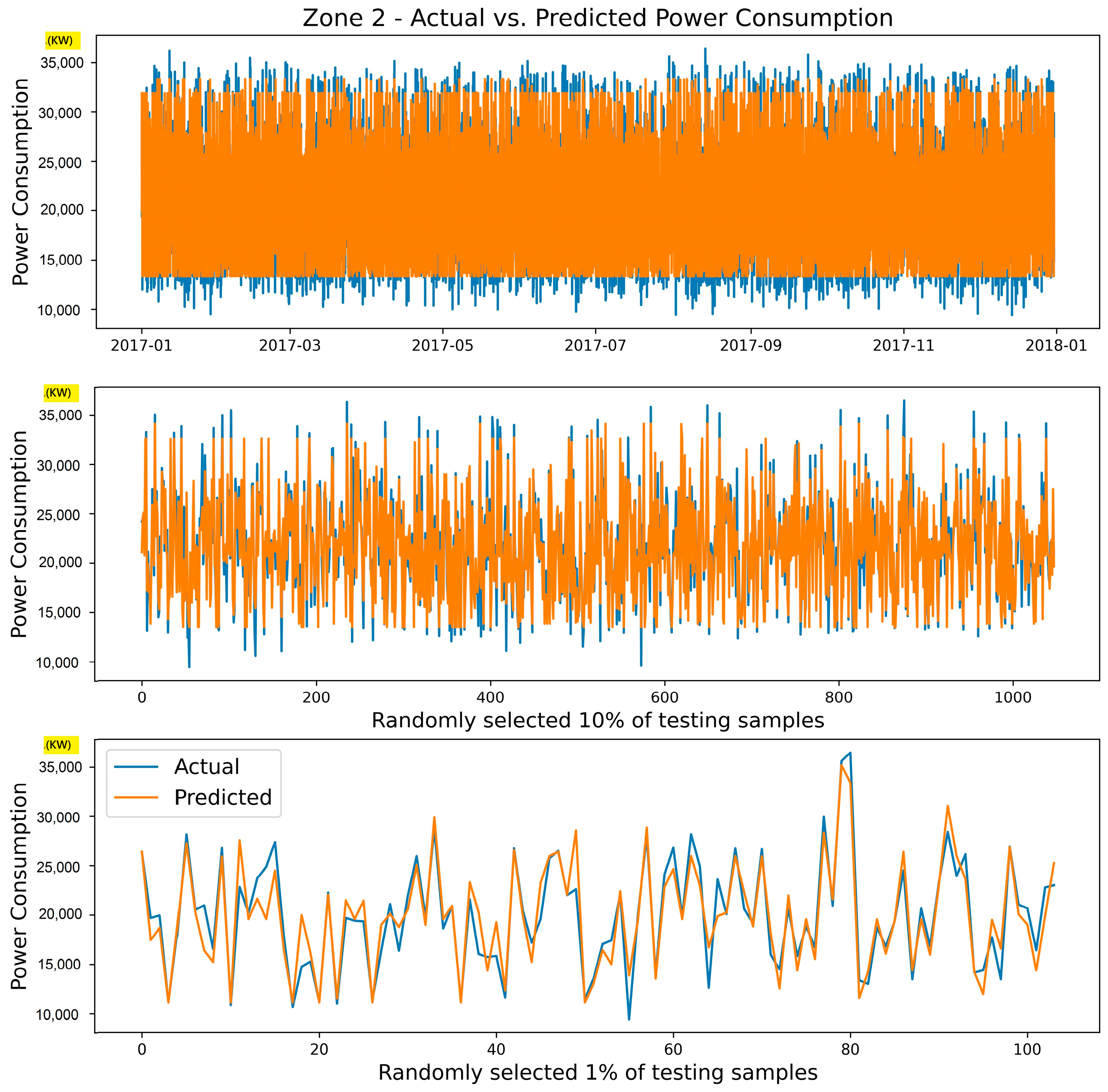
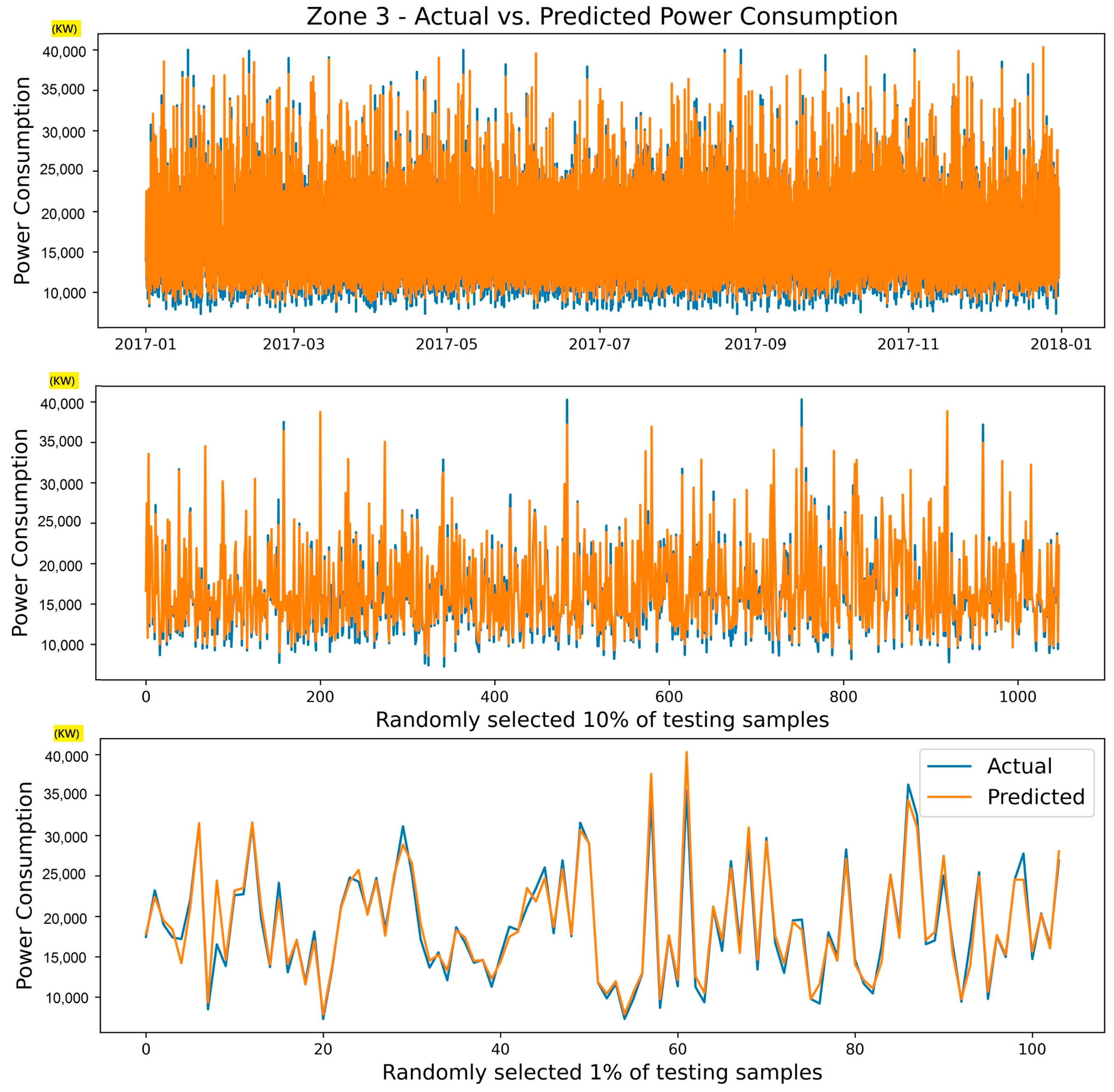
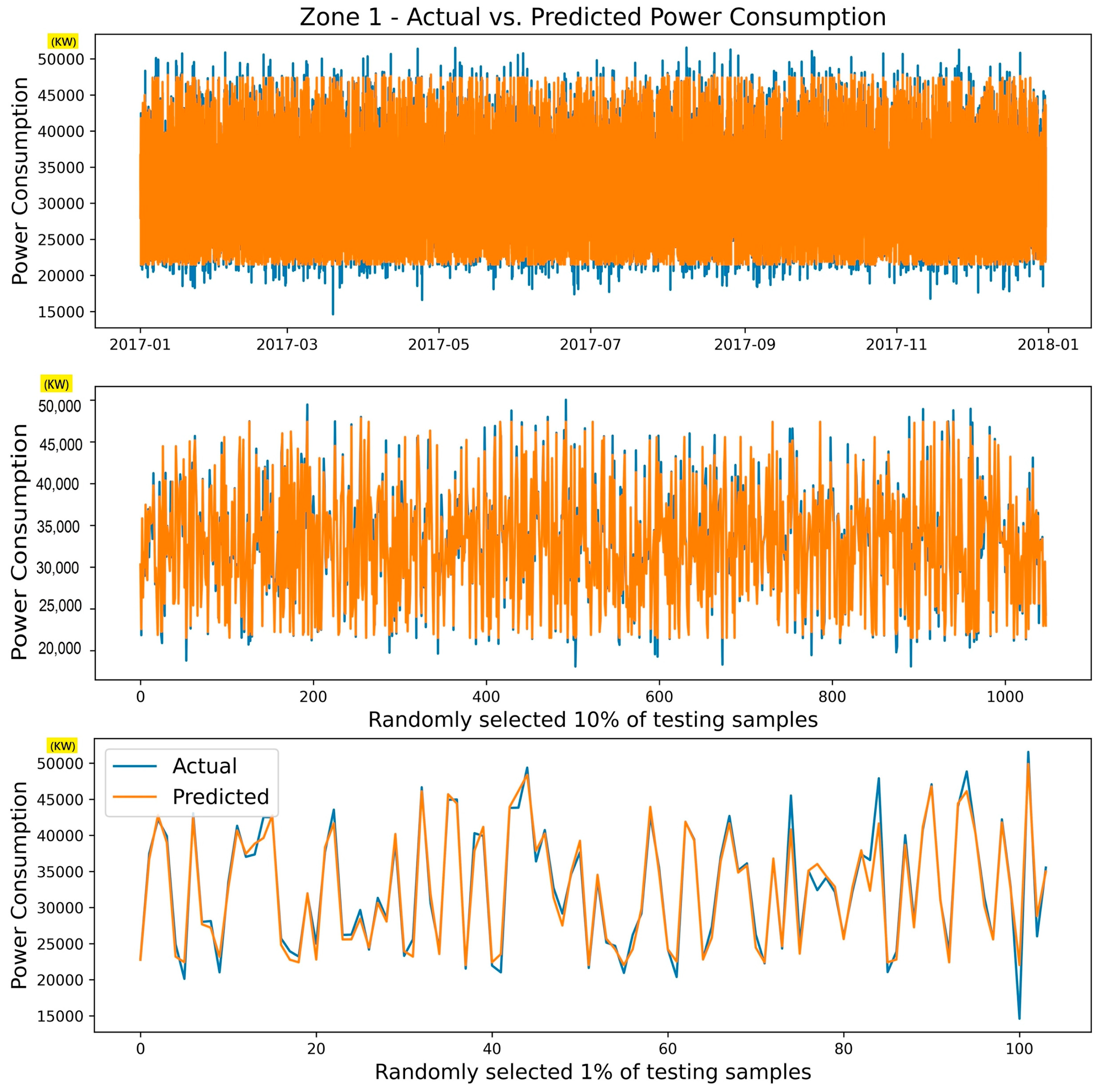
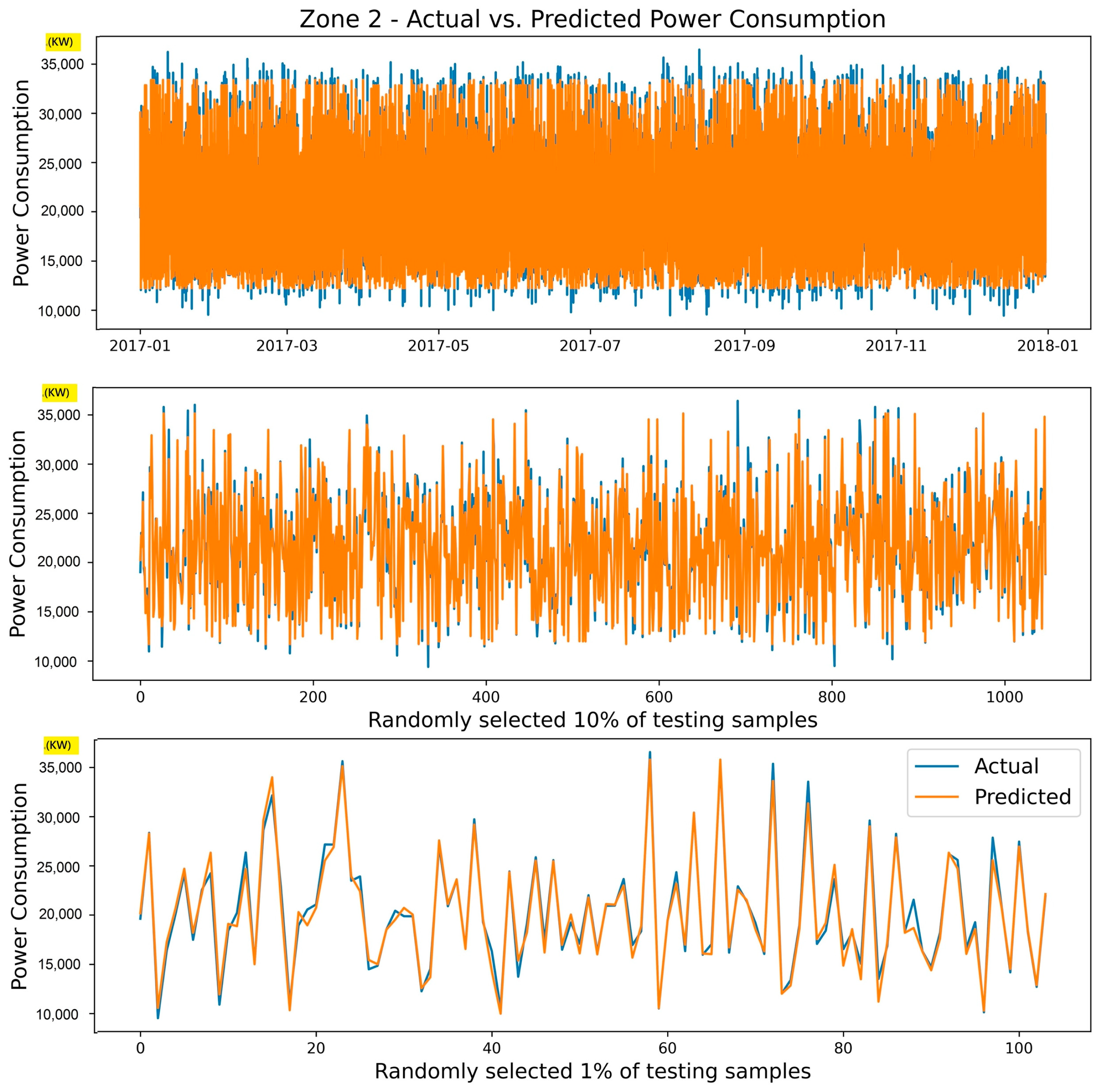
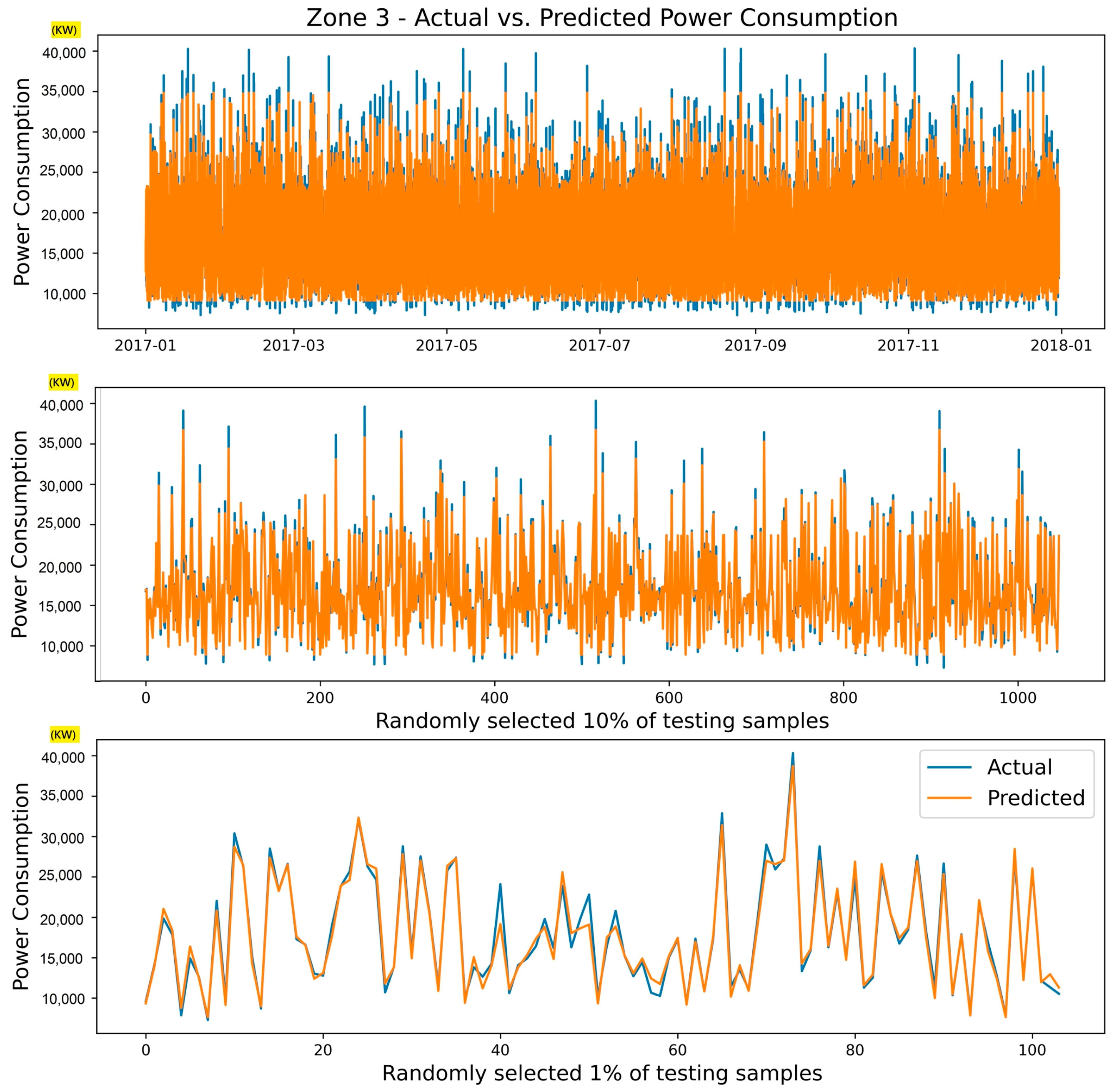
5.3. Prediction with Hyperparameters Optimization

In this experiment, we aim to perform hyperparameter optimization using Randomize Search CV to find the best configuration of hyperparameters for a DL model and to utilize a Keras Regressor wrapper for this purpose. The ‘RandomizedSearchCV’ randomly passes the set of hyperparameters calculates the score and gives the best set of hyperparameters which gives the best score as an output. Cross-validation is a resampling method used to test the model’s generalization ability using out-of-the-sample data chunks. The hybrid framework trains the best model and evaluates its performance on the test data. The components of the optimization process are explained in the following:
(1)
The Keras model architecture consists of two dense layers with specified activation functions, dropout regularization layers, and a final dense layer with one output unit. The model is compiled with the mean squared error loss function and an optimizer, as described above.
(2)
Feature scaling on the input variables using a Standard Scaler which standardizes features by removing the mean and scaling to unit variance.
(3)
Keras Regressor wrapper for compatibility with the hyperparameter tuning algorithm.
(4)
A hyperparameter search space with different settings for the learning rate, dropout rate, number of epochs, batch size, and activation function.
(5)
A Randomized Search CV object from sklearn.model_selection with the Keras Regressor wrapper, the hyperparameter search space, and other parameters like the number of cross-validation folds and scoring metric.
(6)
Hyperparameter optimization using the scaled training data to search for the best combination of hyperparameters based on the specified scoring metric (negative mean squared error).
(7)
Optimal hyperparameters and the corresponding best model from the Randomized Search CV object.
(8)
Train the best model using the scaled training data and the best hyperparameters and lastly make predictions on the scaled test data using the trained best model.
The proposed hybrid model was applied to the power consumption dataset to predict the three targets independently. The hyperparameter search space given to the models includes the following settings: ‘learning rate’: [0.1, 0.01, 0.001], ‘dropout rate’: [0.2, 0.3, 0.4], ‘epochs’: [50, 100, 150], ‘batch size’: [32, 64, 128], and ‘activation’: [‘relu’, ‘sigmoid’]. The optimal parameters that were determined for each experiment are presented in Table 7.
The results obtained are presented in Table 8, demonstrating the advantage of optimizing the model. The table displays the RMSE associated with predicting the power load at its peak point. The prediction accuracy was improved significantly when comparing the results presented in Table 7 and Table 8.
Figure 8, Figure 9 and Figure 10 individually depict the results obtained from the optimized Keres model for Power Consumption prediction across three distinct zones, as defined within our dataset. These figures collectively provide a comprehensive analysis of the model’s predictive capabilities, delivering valuable insights into its performance variations across different zones and sample sizes. Each figure comprises three subfigures: (top) offers a comprehensive overview by displaying results for all testing samples, providing a holistic perspective of the model’s performance over time; (middle) zooms in on a specific subset, precisely 10% of the testing samples, facilitating a more detailed examination of predicted and actual data points; and (bottom) further narrows the focus to a mere 1% of the testing samples, enhancing visual clarity within the plots and enabling meticulous evaluation of the alignment between predicted and actual data points.

5.4. Comparison with Other Models

We performed a comparative analysis by comparing our findings against those of other models designed for the used dataset, as detailed in the scholarly work by Salam and Hibaoui [32]. To evaluate these models comprehensively, we employed the Root-Mean-Squared Error (RMSE) as the established performance criterion. It is worth noting that our model consistently demonstrates superior performance by consistently yielding the lowest RMSE in comparison to the models reported in the existing literature. This compelling evidence underscores the efficacy of our approach and its potential to set a new standard in the field. Table 9 presents the results of different methods applied on the dataset of Tetouan city.

5.5. Potential Limitations

While our proposed hybrid predictive model demonstrated notable advancements in electric LF, it is essential to acknowledge its limitations. Understanding these shortcomings is crucial for refining the model and guiding future research endeavors in this domain.
One of the notable limitations of our model is its sensitivity to specific characteristics of the input data. The model’s performance may vary when applied to datasets with different temporal patterns or levels of noise. Further research is needed to develop techniques that enhance the model’s robustness across diverse datasets. The model’s training and evaluation are based on a dataset obtained from the Distribution Network Station in Tetouan City, Morocco. While our results demonstrate superior performance within this context, generalizing the model to different geographic locations with distinct energy consumption patterns may pose challenges. Future work should explore methods for adapting the model to diverse regional characteristics. Furthermore, the proposed model heavily relies on DL techniques, which may present challenges in terms of interpretability. Interpretability is crucial, especially in applications where decisions impact critical infrastructure. Future research could explore hybrid models that incorporate both DL and interpretable ML techniques to strike a balance between accuracy and interpretability. Furthermore, additional metrics can be used to measuring the peak load prediction error.

6. Conclusions and Future Work

Efficient and accurate LF is crucial for modern power generation facilities to meet dynamic electricity demand. This work highlights the complexity of predicting electricity consumption due to the multifaceted factors influencing energy usage. Consequently, electricity utilities and governmental bodies are actively seeking advanced machine learning solutions to enhance LF.
A hybrid predictive model was designed to enhance the accuracy of multivariate time series forecasting for electricity consumption within the energy domain. The proposed model was compared with other state-of-the-art DL models using a dataset sourced from the Distribution Network Station of Tetouan City in Morocco. In the experiments, we found that a simple and shallow DNN achieved great prediction performance compared to other more complex models introduced in previous studies. In the future, we will focus on validating the accuracy of load-forecasting shallow models by incorporating additional data sources and refining existing algorithms. Exploring new ML techniques and considering factors such as economic indicators, and household lifestyle changes could lead to more precise predictions.
The implications of our research for policymakers are significant in the context of electric LF and the utilization of advanced DL techniques. Our study offers policymakers valuable insights into optimizing energy planning, resource allocation, and grid stability. The enhanced accuracy of our electric LF model can inform decisions related to infrastructure planning and resource optimization, allowing for more efficient deployment of both energy and computational resources. Policymakers can leverage this knowledge to implement measures that ensure a stable and reliable electricity grid, ultimately minimizing the risk of disruptions. Additionally, as the energy landscape evolves towards increased reliance on renewable sources, our findings provide policymakers with guidance on integrating renewable energy into the grid. The introduction of novel DL techniques prompts considerations for supportive policy frameworks that encourage the adoption of advanced technologies in the energy sector. Policymakers can also use the insights from our study to develop strategies that enhance resilience to demand variability, with proactive measures for predicted high-demand periods and the development of adaptive systems. Moreover, the environmental impact of energy generation can be addressed through more efficient energy use facilitated by accurate LF, aligning with sustainability and environmental goals. In summary, our research provides actionable insights for policymakers to shape policies that improve energy management, grid reliability, and environmental sustainability.
The limitations discussed in Section 4.4 open avenues for future research in the field of electric LF. Future investigations should focus on developing models that are more robust across diverse datasets, expanding the geographic applicability of the proposed model, and exploring hybrid approaches that prioritize interpretability without compromising predictive accuracy.

Author Contributions

Conceptualization, H.A.A.-J. and G.M.B.; Methodology, H.A.A.-J., G.M.B., M.Y.W. and M.A.H., Software, H.A.A.-J. and G.M.B., manuscript writing, and revising, H.A.A.-J., G.M.B., M.Y.W. and M.A.H. All authors have read and agreed to the published version of the manuscript.

Funding

This research was funded by Interdisciplinary Research Center for Renewable Energy and Power Systems (IRC-REPS) at KFUPM, grant number INRE2311.

Data Availability Statement

This study utilized a published energy consumption dataset. The dataset has been published and made available for the research community online via the link (https://www.kaggle.com/datasets/fedesoriano/electric-power-consumption/data), accessed date, 15 March 2023.

Acknowledgments

The authors would like to acknowledge the help and support provided by King Fahd University of Petroleum and Minerals (KFUPM). This research was supported by Interdisciplinary Research Center for Renewable Energy and Power Systems (IRC-REPS) at KFUPM in the terms of research.

Conflicts of Interest

The authors declare no conflict of interest.

References

  1. Chen, J.; Liu, M.; Milano, F. Aggregated Model of Virtual Power Plants for Transient Frequency and Voltage Stability Analysis. IEEE Trans. Power Syst. 2021, 36, 4366–4375. [Google Scholar] [CrossRef]
  2. Dewangan, F.; Abdelaziz, A.Y.; Biswal, M. Load Forecasting Models in Smart Grid Using Smart Meter Information: A Review. Energies 2023, 16, 1404. [Google Scholar] [CrossRef]
  3. Muzaffar, S.; Afshari, A. Short-term load forecasts using LSTM networks. Energy Procedia 2019, 158, 2922–2927. [Google Scholar] [CrossRef]
  4. Hammad, M.A.; Jereb, B.; Rosi, B.; Dragan, D. Methods, and Models for Electric Load Forecasting: A Comprehensive Review. Logist. Sustain. Transp. 2020, 11, 51–76. [Google Scholar] [CrossRef]
  5. Zheng, J.; Xu, C.; Zhang, Z.; Li, X. Electric load forecasting in smart grids using long-short-term-memory based recurrent neural network. In Proceedings of the 2017 51st Annual Conference on Information Sciences and Systems (CISS), Baltimore, MD, USA, 22–24 March 2017; pp. 1–6. [Google Scholar]
  6. Singla, M.K.; Nijhawan, P.; Oberoi, A.S.; Singh, P. Application of levenberg marquardt algorithm for short term load forecasting: A theoretical investigation. Pertanika J. Sci. Technol. 2019, 27, 1227–1245. [Google Scholar]
  7. Mehta, S.; Basak, P. A comprehensive review on control techniques for stability improvement in microgrids. Int. Trans. Electr. Energy Syst. 2021, 31, 1–28. [Google Scholar] [CrossRef]
  8. Hou, H.; Liu, C.; Wang, Q.; Wu, X.; Tang, J.; Shi, Y.; Xie, C. Review of load forecasting based on artificial intelligence methodologies, models, and challenges. Electr. Power Syst. Res. 2022, 210, 340–344. [Google Scholar] [CrossRef]
  9. Kong, W.; Dong, Z.Y.; Jia, Y.; Hill, D.J.; Xu, Y.; Zhang, Y. Short-term residential load forecasting based on LSTM recurrent neural network. IEEE Trans. Smart Grid 2017, 10, 841–851. [Google Scholar] [CrossRef]
  10. Li, Z.; Wu, L.; Xu, Y.; Moazeni, S.; Tang, Z. Multi-Stage Real-Time Operation of a Multi-Energy Microgrid with Electrical and Thermal Energy Storage Assets: A Data-Driven MPC-ADP Approach. IEEE Trans. Smart Grid 2022, 13, 213–226. [Google Scholar] [CrossRef]
  11. Tan, M.; Hu, C.; Chen, J.; Wang, L.; Li, Z. Multi-node load forecasting based on multi-task learning with modal feature extraction. Eng. Appl. Artif. Intell. 2022, 112, 104856. [Google Scholar] [CrossRef]
  12. Muhtadi, A.; Pandit, D.; Nguyen, N.; Mitra, J. Distributed Energy Resources Based Microgrid: Review of Architecture, Control, and Reliability. IEEE Trans. Ind. Appl. 2021, 57, 2223–2235. [Google Scholar] [CrossRef]
  13. Conditions and Requirements for the Technical Feasibility of a Power System with a High Share of Renewables in France towards 2050. 2021. Available online: https://www.iea.org/reports/conditions-and-requirements-for-the-technical-feasibility-of-a-power-system-with-a-high-share-of-renewables-in-france-towards-2050 (accessed on 4 June 2023). [CrossRef]
  14. Jacob, M.; Neves, C.; Vukadinović Greetham, D. Forecasting and Assessing Risk of Individual Electricity Peaks; Springer: Cham, Switzerland, 2020. [Google Scholar]
  15. Liu, H.; Xiong, X.; Yang, B.; Cheng, Z.; Shao, K.; Tolba, A. A Power Load Forecasting Method Based on Intelligent Data Analysis. Electronics 2023, 12, 3441. [Google Scholar] [CrossRef]
  16. Almalaq, A.; Edwards, G. A review of deep learning methods applied on load forecasting. In Proceedings of the 2017 16th IEEE International Conference on Machine Learning and Applications (ICMLA), Cancun, Mexico, 18–21 December 2017; pp. 511–516. [Google Scholar]
  17. Proedrou, E. A comprehensive review of residential electricity load profile models. IEEE Access 2021, 9, 12114–12133. [Google Scholar] [CrossRef]
  18. Burg, L.; Gürses-Tran, G.; Madlener, R.; Monti, A. Comparative analysis of load forecasting models for varying time horizons and load aggregation levels. Energies 2021, 14, 7128. [Google Scholar] [CrossRef]
  19. Haben, S.; Arora, S.; Giasemidis, G.; Voss, M.; Greetham, D.V. Review of low voltage load forecasting: Methods, applications, and recommendations. Appl. Energy 2021, 304, 117798. [Google Scholar] [CrossRef]
  20. Vanting, N.; Ma, Z.; Jørgensen, B. A scoping review of deep neural networks for electric load forecasting. Energy Inform. 2021, 4, 49. [Google Scholar] [CrossRef]
  21. Azeem, A.; Ismail, I.; Jameel, S.M.; Harindran, V.R. Electrical load forecasting models for different generation modalities: A review. IEEE Access 2021, 9, 142239–142263. [Google Scholar] [CrossRef]
  22. Mamun, A.A.; Sohel, M.; Mohammad, N.; Sunny, M.S.H.; Dipta, D.R.; Hossain, E. A comprehensive review of the load forecasting techniques using single and hybrid predictive models. IEEE Access 2020, 8, 134911–134939. [Google Scholar] [CrossRef]
  23. Li, J.; Chen, W.; Chen, Y.; Sheng, K.; Du, S.; Zhang, Y.; Wu, Y. A survey on investment demand assessment models for power grid infrastructure. IEEE Access 2021, 9, 9048–9054. [Google Scholar] [CrossRef]
  24. Kuster, C.; Rezgui, Y.; Mourshed, M. Electrical load forecasting models: A critical systematic review. Sustain. Cities Soc. 2017, 35, 257–270. [Google Scholar] [CrossRef]
  25. Hong, T.; Pinson, P.; Wang, Y.; Weron, R.; Yang, D.; Zareipour, H. Energy forecasting: A review and outlook. IEEE Open Access J. Power Energy 2020, 7, 376–388. [Google Scholar] [CrossRef]
  26. Acaroğlu, H.; Márquez, F. Comprehensive review on electricity market price and load forecasting based on wind energy. Energies 2021, 14, 7473. [Google Scholar] [CrossRef]
  27. Ij, H. Statistics versus machine learning. Nat. Methods 2018, 15, 233. [Google Scholar]
  28. Ongsulee, P. Artificial intelligence, machine learning and deep learning. In Proceedings of the 2017 15th International Conference on ICT and Knowledge Engineering (ICT&KE), Bangkok, Thailand, 22–24 November 2017; pp. 1–6. [Google Scholar]
  29. Chahal, A.; Gulia, P. Machine learning and deep learning. Int. J. Innov. Technol. Explor. Eng. 2019, 8, 4910–4914. [Google Scholar]
  30. Dab, K.; Agbossou, K.; Henao, N.; Dubé, Y.; Kelouwani, S.; Hosseini, S.S. A compositional kernel based gaussian process approach to day-ahead residential load forecasting. Energy Build. 2022, 254, 111459. [Google Scholar] [CrossRef]
  31. Syah, R.; Davarpanah, A.; Elveny, M.; Karmaker, A.K.; Nasution, M.K.; Hossain, M.A. Forecasting daily electricity price by hybrid model of fractional wavelet transform, feature selection, support vector machine and optimization algorithm. Electronics 2021, 10, 2214. [Google Scholar] [CrossRef]
  32. Fekri, M.N.; Patel, H.; Grolinger, K.; Sharma, V. Deep learning for load forecasting with smart meter data: Online Adaptive Recurrent Neural Network. Appl. Energy 2021, 282, 116177. [Google Scholar] [CrossRef]
  33. Alrasheedi, A.; Almalaq, A. Hybrid Deep Learning Applied on Saudi Smart Grids for Short-Term Load Forecasting. Mathematics 2022, 10, 2666. [Google Scholar] [CrossRef]
  34. Goodfellow, I.; Bengio, Y.; Courville, A. Deep Learning; MIT Press: Cambridge, MA, USA, 2016. [Google Scholar]
  35. Langdon, W.B.; Gustafson, S.M. Genetic programming, and evolvable machines: Ten years of reviews. Genet. Progr. Evol. Mach. 2010, 11, 321–338. [Google Scholar] [CrossRef]
  36. Akhtar, S.; Adeel, M.; Iqbal, M.; Namoun, A.; Tufail, A.; Kim, K.-H. Deep learning methods utilization in electric power systems. Energy Rep. 2023, 10, 2138–2151. [Google Scholar] [CrossRef]
  37. Abdulrahman, M.L.; Ibrahim, K.M.; Gital, A.Y.; Zambuk, F.U.; Ja’afaru, B.; Yakubu, Z.I.; Ibrahim, A. A review on deep learning with focus on deep recurrent neural network for electricity forecasting in residential building. Procedia Comput. Sci. 2021, 193, 141–154. [Google Scholar] [CrossRef]
  38. Dong, Y.; Ma, X.; Fu, T. Electrical load forecasting: A deep learning approach based on K-nearest neighbors. Appl. Soft Comput. 2021, 99, 106900. [Google Scholar] [CrossRef]
  39. Farsi, B.; Amayri, M.; Bouguila, N.; Eicker, U. On short-term load forecasting using machine learning techniques and a novel parallel deep LSTM-CNN approach. IEEE Access 2021, 9, 31191–31212. [Google Scholar] [CrossRef]
  40. Kouvelas, V.; Moschakis, M. Short-term Electric Load Forecasting using Engineering and Deep Learning techniques. In Proceedings of the 2022 2nd International Conference on Energy Transition in the Mediterranean Area (SyNERGY MED), Thessaloniki, Greece, 17–19 October 2022; pp. 1–5. [Google Scholar] [CrossRef]
  41. Liu, F.; Dong, T.; Liu, Q.; Liu, Y.; Li, S. Combining fuzzy clustering and improved long short-term memory neural networks for short-term load forecasting. Electr. Power Syst. Res. 2024, 226, 109967. [Google Scholar] [CrossRef]
  42. Zeyu, W.; Yueren, W.; Rouchen, Z.; Srinivasan, R.S.; Ahrentzen, S. Random Forest based hourly building energy prediction. Energy Build. 2018, 171, 11–25. [Google Scholar]
  43. Touzani, S.; Granderson, J.; Fernandes, S. Gradient boosting machine for modelling the energy consumption of commercial buildings. Energy Build. 2018, 158, 1533–1543. [Google Scholar] [CrossRef]
  44. Hadri, S.; Naitmalek, Y.; Najib, M.; Bakhouya, M.; Fakhiri, Y.; Elaroussi, M. A Comparative Study of Predictive Approaches for Load Forecasting in Smart Buildings. Procedia Comput. Sci. 2019, 160, 173–180. [Google Scholar] [CrossRef]
  45. Vrablecová, P.; Bou Ezzeddine, A.; Rozinajová, V.; Šárik, S.; Sangaiah, A.K. Smart grid load forecasting using online support vector regression. Comput. Electr. Eng. 2018, 65, 102–117. [Google Scholar] [CrossRef]
  46. Khan, S.; Javaid, N.; Chand, A.; Khan, A.B.M.; Rashid, F.; Afridi, I.U. Electricity Load Forecasting for Each Day of Week Using Deep CNN. Adv. Intell. Syst. Comput. 2019, 927, 1107–1119. [Google Scholar]
  47. Chen, S.; Ren, Y.; Friedrich, D.; Yu, Z.; Yu, J. Prediction of office building electricity demand using artificial neural network by splitting the time horizon for different occupancy rates. Energy AI 2021, 5, 100093. [Google Scholar] [CrossRef]
  48. Amber, K.P.; Ahmad, R.; Aslam, M.W.; Kousar, A.; Usman, M.; Khan, M.S. Intelligent techniques for forecasting electricity consumption of buildings. Energy 2018, 157, 886–893. [Google Scholar] [CrossRef]
  49. Zhong, H.; Wang, J.; Jia, H.; Mu, Y.; Lv, S. Vector field-based support vector regression for building energy consumption prediction. Appl. Energy 2019, 242, 403–414. [Google Scholar] [CrossRef]
  50. Martínez-Comesaña, M.; Febrero-Garrido, M.; Granada-Álvarez, E.; Martínez-Torres, J.; Martínez-Mariño, S. Heat Loss Coefficient Estimation Applied to Existing Buildings through Machine Learning Models. Appl. Sci. 2020, 10, 8968. [Google Scholar] [CrossRef]
  51. Al-Gabalawy, M.; Hosny, N.S.; Adly, A.R. Probabilistic forecasting for energy time series considering uncertainties based on deep learning algorithms. Electr. Power Syst. Res. 2021, 196, 107216. [Google Scholar] [CrossRef]
  52. Guo, J.; Lin, P.; Zhang, L.; Pan, Y.; Xiao, Z. Dynamic adaptive encoder-decoder deep learning networks for multivariate time series forecasting of building energy consumption. Appl. Energy 2023, 350, 121803. [Google Scholar] [CrossRef]
  53. Chen, Q.; Zhang, W.; Zhu, K.; Zhou, D.; Dai, H.; Wu, Q. A novel trilinear deep residual network with self-adaptive dropout method for short-term load forecasting. Expert Syst. Appl. 2021, 182, 115272. [Google Scholar] [CrossRef]
  54. Somu, N.; MR, G.R.; Ramamritham, K. A deep learning framework for building energy consumption forecast. Renew. Sustain. Energy Rev. 2021, 137, 110591. [Google Scholar] [CrossRef]
  55. Mughees, N.; Mohsin, S.A.; Mughees, A.; Mughees, A. Deep sequence to sequence Bi-LSTM neural networks for day-ahead peak load forecasting. Expert Syst. Appl. 2021, 175, 114844. [Google Scholar] [CrossRef]
  56. Wang, T.; Lai, C.S.; Ng, W.W.; Pan, K.; Zhang, M.; Vaccaro, A.; Lai, L.L. Deep autoencoder with localized stochastic sensitivity for short-term load forecasting. Int. J. Electr. Power Energy Syst. 2021, 130, 106954. [Google Scholar] [CrossRef]
  57. Vaygan, E.K.; Rajabi, R.; Estebsari, A. Short-term load forecasting using time pooling deep recurrent neural network. In Proceedings of the 2021 IEEE International Conference on Environment and Electrical Engineering and 2021 IEEE Industrial and Commercial Power Systems Europe (EEEIC/I&CPS Europe), Bari, Italy, 7–10 September 2021; pp. 1–5. [Google Scholar]
  58. Hu, Y.; Qu, B.; Wang, J.; Liang, J.; Wang, Y.; Yu, K.; Li, Y.; Qiao, K. Short-term load forecasting using multimodal evolutionary algorithm and random vector functional link network-based ensemble learning. Appl. Energy 2021, 285, 116415. [Google Scholar] [CrossRef]
  59. Zhang, W.; Chen, Q.; Yan, J.; Zhang, S.; Xu, J. A novel asynchronous deep reinforcement learning model with adaptive early forecasting method and reward incentive mechanism for short-term load forecasting. Energy 2021, 236, 121492. [Google Scholar] [CrossRef]
  60. Thejus, S.; Sivraj, P. Deep learning-based power consumption and generation forecasting for demand side management. In Proceedings of the 2021 Second International Conference on Electronics and Sustainable Communication Systems (ICESC), Coimbatore, India, 4–6 August 2021; pp. 1350–1357. [Google Scholar]
  61. Wang, J.; Chen, X.; Zhang, F.; Chen, F.; Xin, Y. Building load forecasting using deep neural network with efficient feature fusion. J. Mod. Power Syst. Clean. Energy 2021, 9, 160–169. [Google Scholar] [CrossRef]
  62. Irankhah, A.; Rezazadeh, S.; Moghaddam, M.H.Y.; Ershadi-Nasab, S. Hybrid deep learning method based on lstm-autoencoder network for household short-term load forecasting. In Proceedings of the 2021 7th International Conference on Signal Processing and Intelligent Systems (ICSPIS), Tehran, Iran, 29–30 December 2021; pp. 1–6. [Google Scholar]
  63. Sinha, A.; Sawant, M.; Kochar, H.; Abhija, A.; Seth, R.; Sornagattu, P.R.; Vyas, O. Demand response optimization for microgrid clusters with deep reinforcement learning. In Proceedings of the 2021 12th International Conference on Computing Communication and Networking Technologies (ICCCNT), Kharagpur, India, 6–8 July 2021; pp. 1–7. [Google Scholar]
  64. Mansoor, H.; Rauf, H.; Mubashar, M.; Khalid, M.; Arshad, N. Past vector similarity for short term electrical load forecasting at the individual household level. IEEE Access 2021, 9, 42771–42785. [Google Scholar] [CrossRef]
  65. Shabbir, N.; Kütt, L.; Raja, H.A.; Ahmadiahangar, R.; Rosin, A.; Husev, O. Machine learning and deep learning techniques for residential load forecasting: A comparative analysis. In Proceedings of the 2021 IEEE 62nd International Scientific Conference on Power and Electrical Engineering of Riga Technical University (RTUCON), Riga, Latvia 15–17 November 2021; pp. 1–5. [Google Scholar]
  66. Li, Y.; Wang, R.; Yang, Z. Optimal scheduling of isolated microgrids using automated reinforcement learning-based multi-period forecasting. IEEE Trans. Sustain. Energy 2021, 13, 159–169. [Google Scholar] [CrossRef]
  67. Ibrahim, N.M.; Megahed, A.I.; Abbasy, N.H. Short-term individual household load forecasting framework using LSTM deep learning approach. In Proceedings of the 2021 5th International Symposium on Multidisciplinary Studies and Innovative Technologies (ISMSIT), Ankara, Turkey, 21–23 October 2021; pp. 257–262. [Google Scholar]
  68. Cheng, L.; Zang, H.; Xu, Y.; Wei, Z.; Sun, G. Probabilistic residential load forecasting based on micrometeorological data and customer consumption pattern. IEEE Trans. Power Syst. 2021, 36, 3762–3775. [Google Scholar] [CrossRef]
  69. He, Y.; Luo, F.; Ranzi, G.; Kong, W. Short-term residential load forecasting based on federated learning and load clustering. In Proceedings of the 2021 IEEE International Conference on Communications, Control, and Computing Technologies for Smart Grids (SmartGridComm), Aachen, Germany, 25–28 October 2021; pp. 77–82. [Google Scholar]
  70. Bento, P.M.; Pombo, J.A.; Calado, M.R.; Mariano, S.J. Stacking ensemble methodology using deep learning and ARIMA models for short-term load forecasting. Energies 2021, 14, 7378. [Google Scholar] [CrossRef]
  71. Salman, D.; Kusaf, M.; Elmi, Y.K. Using recurrent neural network to forecast day and year ahead performance of load demand: A case study of France. In Proceedings of the 2021 10th International Conference on Power Science and Engineering (ICPSE), Istanbul, Turkey, 21–23 October 2021; pp. 23–30. [Google Scholar]
  72. Yaprakdal, F. An ensemble deep-learning-based model for hour-ahead load forecasting with a feature selection approach: A comparative study with state-of-the-art methods. Energies 2022, 16, 57. [Google Scholar] [CrossRef]
  73. Zhang, G.; Bai, X.; Wang, Y. Short-time multi-energy load forecasting method based on CNN-Seq2Seq model with attention mechanism. Mach. Learn. Appl. 2021, 5, 100064. [Google Scholar] [CrossRef]
  74. Fekri, M.N.; Grolinger, K.; Mir, S. Distributed load forecasting using smart meter data: Federated learning with Recurrent Neural Networks. Int. J. Electr. Power Energy Syst. 2022, 137, 107669. [Google Scholar] [CrossRef]
  75. Lu, Y.; Wang, G.; Huang, S. A short-term load forecasting model based on mixup and transfer learning. Electr. Power Syst. Res. 2022, 207, 107837. [Google Scholar] [CrossRef]
  76. Ahajjam, M.A.; Licea, D.B.; Ghogho, M.; Kobbane, A. Experimental investigation of variational mode decomposition and deep learning for short-term multi-horizon residential electric load forecasting. Appl. Energy 2022, 326, 119963. [Google Scholar] [CrossRef]
  77. Hadjout, D.; Torres, J.; Troncoso, A.; Sebaa, A.; Martínez-Álvarez, F. Electricity consumption forecasting based on ensemble deep learning with application to the Algerian market. Energy 2022, 243, 123060. [Google Scholar] [CrossRef]
  78. Abdel-Basset, M.; Hawash, H.; Sallam, K.; Askar, S.; Abouhawwash, M. STLFNet: Two-stream deep network for short-term load forecasting in residential buildings. J. King Saud. Univ-Comput. Inf. Sci. 2022, 34, 4296–4311. [Google Scholar]
  79. Fernández, J.D.; Menci, S.P.; Lee, C.M.; Rieger, A.; Fridgen, G. Privacy-preserving federated learning for residential short-term load forecasting. Appl. Energy 2022, 326, 119915. [Google Scholar] [CrossRef]
  80. Javed, U.; Ijaz, K.; Jawad, M.; Khosa, I.; Ansari, E.A.; Zaidi, K.S.; Rafiq, M.N.; Shabbir, N. A novel short receptive field based dilated causal convolutional network integrated with bidirectional LSTM for short-term load forecasting. Expert Syst. Appl. 2022, 205, 117689. [Google Scholar] [CrossRef]
  81. Aouad, M.; Hajj, H.; Shaban, K.; Jabr, R.A.; El-Hajj, W. A CNN-sequence-to-sequence network with attention for residential short-term load forecasting. Electr. Power Syst. Res. 2022, 211, 108152. [Google Scholar] [CrossRef]
  82. Sharma, A.; Jain, S.K. A novel seasonal segmentation approach for day-ahead load forecasting. Energy 2022, 257, 124752. [Google Scholar] [CrossRef]
  83. Yang, W.; Shi, J.; Li, S.; Song, Z.; Zhang, Z.; Chen, Z. A combined deep learning load forecasting model of single household resident user considering multi-time scale electricity consumption behavior. Appl. Energy 2022, 307, 118197. [Google Scholar] [CrossRef]
  84. Reddy, S.; Akashdeep, S.; Harshvardhan, R.; Kamath, S. Stacking deep learning and machine learning models for short-term energy consumption forecasting. Adv. Eng. Inform. 2022, 52, 101542. [Google Scholar]
  85. Xiao, X.; Mo, H.; Zhang, Y.; Shan, G. Meta-ANN–A dynamic artificial neural network refined by meta-learning for Short-Term Load Forecasting. Energy 2022, 246, 123418. [Google Scholar] [CrossRef]
  86. Yan, K.; Zhou, X.; Chen, J. Collaborative deep learning framework on IoT data with bidirectional NLSTM neural networks for energy consumption forecasting. J. Parallel Distrib. Comput. 2022, 163, 248–255. [Google Scholar] [CrossRef]
  87. Abdallah, M.; Talib, M.A.; Hosny, M.; Waraga, O.A.; Nasir, Q.; Arshad, M.A. Forecasting highly fluctuating electricity load using machine learning models based on multimillion observations. Adv. Eng. Inform. 2022, 53, 101707. [Google Scholar] [CrossRef]
  88. Tong, X.; Wang, J.; Zhang, C.; Wu, T.; Wang, H.; Wang, Y. LS-LSTM-AE: Power load forecasting via long-short series features and LSTM-autoencoder. Energy Rep. 2022, 8, 596–603. [Google Scholar] [CrossRef]
  89. Deng, X.; Ye, A.; Zhong, J.; Xu, D.; Yang, W.; Song, Z.; Zhang, Z.; Guo, J.; Wang, T.; Tian, Y.; et al. Bagging–XGBoost algorithm based extreme weather identification and short-term load forecasting model. Energy Rep. 2022, 8, 8661–8674. [Google Scholar] [CrossRef]
  90. Inteha, A.; Hussain, F.; Khan, I.A. A data driven approach for day ahead short-term load forecasting. IEEE Access 2022, 10, 84227–84243. [Google Scholar] [CrossRef]
  91. Moradzadeh, A.; Moayyed, H.; Zare, K.; Mohammadi-Ivatloo, B. Short-term electricity demand forecasting via variational autoencoders and batch training based bidirectional long short-term memory. Sustain. Energy Technol. Assess. 2022, 52, 102209. [Google Scholar] [CrossRef]
  92. Liu, M.; Sun, X.; Wang, Q.; Deng, S. Short-term load forecasting using EMD with feature selection and TCN-based deep learning model. Energies 2022, 15, 7170. [Google Scholar] [CrossRef]
  93. Ibrahim, B.; Rabelo, L.; Gutierrez-Franco, E.; Clavijo-Buritica, N. Machine learning for short-term load forecasting in smart grids. Energies 2022, 15, 8079. [Google Scholar] [CrossRef]
  94. Taleb, I.; Guerard, G.; Fauberteau, F.; Nguyen, N. A flexible deep learning method for energy forecasting. Energies 2022, 15, 3926. [Google Scholar] [CrossRef]
  95. Alotaibi, M.A. Machine learning approach for short-term load forecasting using deep neural network. Energies 2022, 15, 6261. [Google Scholar] [CrossRef]
  96. Luo, X.; Oyedele, L.O. A self-adaptive deep learning model for building electricity load prediction with moving horizon. Mach. Learn. Appl. 2022, 7, 100257. [Google Scholar] [CrossRef]
  97. Zou, Y.; Feng, W.; Zhang, J.; Li, J. Forecasting of short-term load using the MFF-SAM-GCN model. Energies 2022, 15, 3140. [Google Scholar] [CrossRef]
  98. Akhtar, S.; Shahzad, S.; Zaheer, A.; Ullah, H.S.; Kilic, H.; Gono, R.; Jasiński, M.; Leonowicz, Z. Short-term load forecasting models: A review of challenges, progress, and the road ahead. Energies 2023, 16, 4060. [Google Scholar] [CrossRef]
  99. Arnold, T.B. kerasR: R Interface to the Keras Deep Learning Library. J. Open Source Softw. 2017, 2, 296. [Google Scholar] [CrossRef]
  100. Ketkar, N.; Ketkar, N. Introduction to keras. In Deep Learning with Python a Hands-on Introd; Apress: Berkeley, CA, USA, 2017; pp. 97–111. [Google Scholar] [CrossRef]
  101. Tarek, H.; Aly, H.; Eisa, S.; Abul-Soud, M. Optimized deep learning algorithms for tomato leaf disease detection with hardware deployment. Electronics 2022, 11, 140. [Google Scholar] [CrossRef]
  102. Konar, J.; Khandelwal, P.; Tripathi, R. Comparison of various learning rate scheduling techniques on convolutional neural network. In Proceedings of the 2020 IEEE International Students’ Conference on Electrical, Electronics and Computer Science (SCEECS), Bhopal, India, 22–23 February 2020; pp. 1–5. [Google Scholar]
  103. Al-Kababji, A.; Bensaali, F.; Dakua, S.P. Scheduling techniques for liver segmentation: Reducelronplateau vs. onecyclelr. In Proceedings of the International Conference on Intelligent Systems and Pattern Recognition; Springer: Berlin/Heidelberg, Germany, 2022; pp. 204–212. [Google Scholar]
  104. Bisong, E.; Bisong, E. Regularization for deep learning. In Building Machine Learning and Deep Learning Models on Google Cloud Platform: A Comprehensive Guide for Beginners; Apress: Berkeley, CA, USA, 2019; pp. 415–421. ISBN 9781484244708. [Google Scholar]
  105. Dekel, O.; Gilad-Bachrach, R.; Shamir, O.; Xiao, L. Optimal Distributed Online Prediction Using Mini-Batches. J. Mach. Learn. Res. 2012, 13, 165–202. [Google Scholar]
  106. Liu, Y.; Dou, S.; Du, Y.; Wang, Z. Gearbox Fault Diagnosis Based on Gramian Angular Field and CSKD-ResNeXt. Electronics 2023, 12, 2475. [Google Scholar] [CrossRef]
  107. Salam, A.; El Hibaoui, A. Energy consumption prediction model with deep inception residual network inspiration and LSTM. Math. Comput. Simul. 2021, 190, 97–109. [Google Scholar] [CrossRef]
Figure 1. Data feature distribution analysis using violin plot.
Electronics 12 04909 g001
Figure 2. Box plot analysis of the power consumption of the three zones.
Electronics 12 04909 g002
Figure 3. Pearson’s correlation coefficient matrix comparing the dataset variables. Positive correlations are colored dark blue; negative correlations are light. The scale down the side of the graphic depicts the gradient of the correlation’s strength and weakness from +1 to −1.
Electronics 12 04909 g003
Figure 4. Methodology flowchart.
Electronics 12 04909 g004
Figure 5. Zone-1 power consumption prediction over time using the Keres model. (top) All testing samples, (middle) with 10% of testing samples, and (bottom) 1% of testing samples.
Electronics 12 04909 g005
Figure 6. Zone-2 power consumption prediction over time using the Keres model: (top) all testing samples, (middle) with 10% of testing samples, and (bottom) 1% of testing samples.
Electronics 12 04909 g006
Figure 7. Zone-3 power consumption prediction over time using the Keres model. (top) All testing samples, (middle) with 10% of testing samples, and (bottom) 1% of testing samples.
Electronics 12 04909 g007
Figure 8. Zone-1 power consumption prediction over time using the optimized Keres model (top) all testing samples, (middle) with 10% of testing samples, (bottom) 1% of testing samples.
Electronics 12 04909 g008
Figure 9. Zone-2 power consumption prediction over time using the optimized Keres model (top) all testing samples, (middle) with 10% of testing samples, (bottom) 1% of testing samples.
Electronics 12 04909 g009
Figure 10. Zone-3 power consumption prediction over time using the optimized Keres model (top) all testing samples, (middle) with 10% of testing samples, (bottom) 1% of testing samples.
Electronics 12 04909 g010
Table 1. Summary of the most recent related work.
Proposed Technique(s)Main ObjectiveRef.Year
Trilinear deep residual network with self-adaptive dropout method based on hierarchical clustering and Gaussian noise.To put forth a resilient model that addresses challenges related to vanishing and exploding gradients, tackles overfitting concerns, and concurrently enhances forecasting accuracy.[51]2021
Hybrid interval forecasting model combining k-NN optimized by genetic algorithm (GA), DBN and self-adaptive kernel density estimation techniquesTo showcase the effectiveness of the proposed interval forecasting model in terms of precision and adaptability, all while maintaining the simplicity of the forecasting procedures.[52]2021
Online adaptive RNNTo achieve higher accuracy than the stand-alone offline LSTM network[53]2021
The algorithms of concrete dropouts, deep ensembles, Bayesian NNs, deep Gaussian processes, and functional neural processesTo delve into the probabilistic extensions and performance capabilities of DL algorithms.[54]2021
Non-linear fully connected feed-forward ANN by autoencoder with localized stochastic sensitivityTo suggest a DL model with the primary goal of improving prediction accuracy and reliability by minimizing errors, which are characterized by the training error and stochastic sensitivity.[55]2021
k-means CNN-LSTM forecast model with clustering approachTo acquire dependable energy consumption data for an academic building, specifically for Demand Response (DR) application purposes.[56]2021
Asynchronous deep reinforcement learning (RL) based model with deterministic policy gradientTo tackle the challenges of high temporal correlation and convergence instability in STLF by employing a deep RL model.[57]2021
Bidirectional LSTM based sequence to sequence regression approachTo assess the effectiveness of the proposed model by comparing it with other competitive techniques on both public holidays and regular days, considering factors such as accuracy and its performance under conditions of limited data availability.[58]2021
Ensemble learning model using multi-modal multi-objective evolutionary algorithm and random vector functional link network-based ensemble learningTo uncover additional trade-off multimodal solutions by leveraging the mapping capabilities of the proposed ensemble learning approach within the context of STLF problems.[59]2021
CNNTo improve the model’s capability to capture non-linear relationships, a proposed feature selection process is introduced.[60]2021
Deep RNNTo enhance forecasting accuracy and performance, especially in the presence of uncertain model dynamics.[61]2021
Deep RLTo contemplate the utilization of a pre-trained dataset, as opposed to a random one, when presenting LF results with the aim of optimizing DR applications.[62]2021
RNN, vanilla LSTM, stacked LSTM, bidirectional LSTM and GRUTo assess the performance of LF, a comparative analysis is conducted involving RNN, three different variants of the LSTM model, and GRU.[63]2021
A prioritized experience replay automated RLTo provide a coupled approach with multi period forecasting and DR program.[64]2021
Hybrid network consisted the layers of autoencoder LSTM, bidirectional LSTM, and stack of LSTMTo showcase the superior performance of the proposed hybrid model when tested with a dataset collected from a residential home, in comparison to previous studies with similar objectives.[65]2021
Comparative analysis with linear regression, tree-based regression, linear support vector machine (SVM), quadratic SVM, cubic SVM and RNNTo evaluate the performance of various ML and DL-based residential LF models.[66]2021
CNN with squeeze-and-excitation modulesTo depict the robust relationship between climate variables and the volatile load demand in residential settings through the proposed model.[67]2021
Past vector similarityTo predict the load at a finer granularity by extracting precise load patterns associated with the occupants’ routines and socio-economic values.[68]2021
RNN with LSTMTo evaluate the predictive performance of the proposed model in comparison to other models utilizing the same dataset.[69]2021
Separate use of LSTM and GRUTo show that the accuracy performance of STLF better than the longer focused forecasting models.[70]2021
Residential LF framework combined by k-means clustering algorithm and federated learningTo institute a collaborative training procedure by leveraging fine-grained monitored consumption data.[71]2021
CNN sequence to sequence model with an attention mechanism based on a multi-task learning methodTo demonstrate the superior accuracy performance of the proposed model.[72]2021
Deep forward NN by automated selecting the best Box–Jenkins modelsTo obtain higher accuracy than the shallow networks.[73]2021
LSTM by mix-up and transfer learning techniquesTo suggest a dependable model by considering the shortage of sufficient historical data on consumption, a factor that diminishes accuracy.[74]2022
Backward-eliminated exhaustive ensemble model for future selection method, and the LF techniques of k-NN, CNN, RNN and SVR.To achieve higher accuracy, the proposal includes a backward-eliminated exhaustive approach for the feature selection technique.[75]2022
Ensemble model with LSTM, GRU, and TCNTo illustrate that the ensemble models proposed exhibit superior performance compared to traditional individual models.[76]2022
LSTM, federated stochastic gradient descent and federated averaging.To train a single federated learning-based model when dealing with multiple smart meters, thereby eliminating the necessity of sharing local data.[77]2022
Federated learning model with ANN architectureTo meet the privacy and security requirements for residential LF by considering the dynamic power demand data from smart meters.[78]2022
CNN based on wavelet and varying mode decompositionTo extract more detailed spectral and temporal information to improve forecasting performance, particularly in situations where exogenous data are unavailable.[79]2022
Hybrid model including the CNN and an attention-based sequence to sequence network.To enhance the forecasting performance by capturing the long-term spatial and temporal features inherent in the data.[80]2022
Consecutive applications of STLF network with a layer of GRUs and STLF network constructed by stacking several TCNsTo improve the DL-based elastic model, ensuring robust performance under diverse conditions, such as variations in accommodation, temperature, humidity, and wind speed.[81]2022
Ensemble structure based on LSTM and XGBoostTo suggest a more accurate and scalable model, aimed at alleviating some of the limitations present in current approaches.[82]2022
Two stage encoder-decoder architecture based on receptive field-based dilated causal convolutional and bidirectional LSTM networks.To increase the STLF performance by encoder–decoder configuration.[83]2022
A dynamic ANN model motivated by meta-learningTo introduce a fine-tuning approach for predicting highly non-stationary points, aiming to implement a robust forecasting procedure.[84]2022
LSTM with back propagation NN and XGBoostTo seek a balanced solution to the trade-off between forecasting accuracy and computational speed.[85]2022
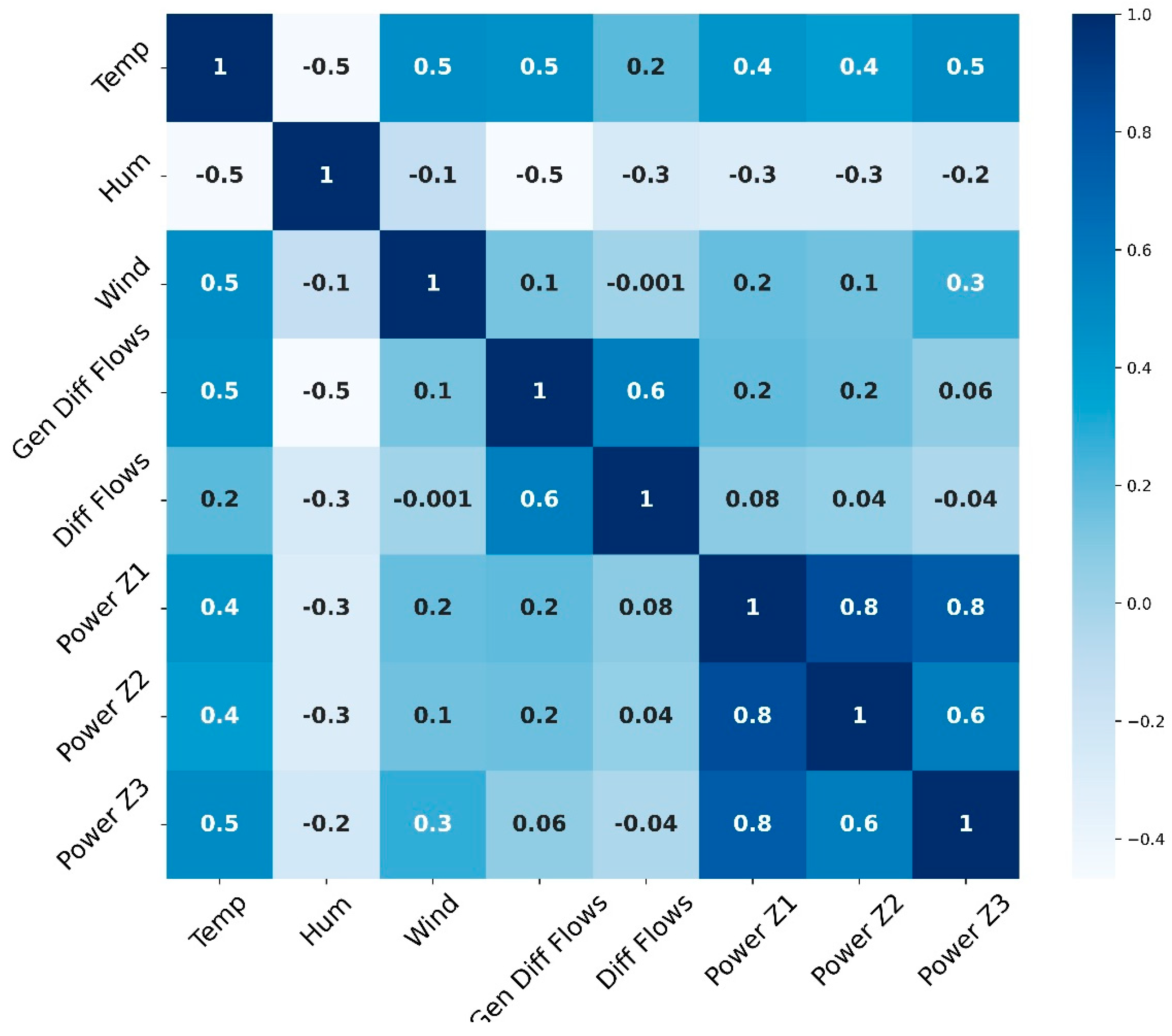
Ensemble model with XGBoost and light-gradient boosting machine (GBM), RF regression and stacking regressorTo analyze the correlation between various variables in the dataset and assess the model performance with a focus on the most influential variables.[86]2022
Bidirectional LSTMTo suggest seasonal segmentation as a strategy to achieve relatively higher accuracy in the forecasting procedure. This approach considers the seasonal factors specific to the dataset of the geographical territory, enhancing the precision of predictions.[87]2022
A multi-channel bidirectional nested LSTM frameworkTo improve the prediction accuracy by following multiple sub-signal processing approach.[88]2022
XGBoostTo determine the occurrence range of peak load considering the load, weather and time factors.[89]2022
Hybrid model called as variational autoencoder bidirectional LSTMTo demonstrate the effectiveness of the proposed method compared to classical models.[90]2022
Autoencoder based LSTMTo introduce a dual-channel structure in the encoder section to extract various levels of time series data. Furthermore, a three-channel output structure in the decoder part is recommended to augment the model’s representation ability.[91]2022
ML models of SVR, RF, XGBoost, light-GBM, adaptive boosting, bidirectional LSTM, GRU, and a DL regression model.To specify best features and searching for nest ML model for predicting the hourly demand.[92]2022
Hybrid model with integrated GA bidirectional GRUTo introduce a more stable and reliable model compared to models developed using classical methods.[93]2022
ML approach with deep ANN and decision tree-based predictionTo show that the ML algorithms and regression analysis have adequate accuracy for LF.[94]2022
Hybrid structure with empirical mode decomposition, one-dimensional CNN, TCN, a self-attention mechanism, and a LSTMTo propose hybrid model having more stable and accurate prediction for STLF problem.[95]2022
Joint structure with multi-feature fusion, self-attention mechanism, convolutional graph networkTo obtain better prediction performance than some of the benchmark models.[96]2022
Hybrid structure with CNN, LSTM and MLPTo propose a solution that offers both adequate accuracy and robustness for LF problems.[97]2022
A self-adaptive DL model with particle swarm optimization (PSO)To enhance the accuracy, robustness, repeatability, and self-adaptive capability in load prediction.[98]2022
Table 2. Statistical analysis of the descriptors and target.
MeanSTDMaximumMinimumSkewnessKurtosis
Temperature (°C)18.815.8240.013.2470.197−0.303
Humidity (g·m−3)68.2615.5694.811.34−0.625−0.122
Wind Speed (m/s)1.962.356.480.050.462−1.783
General Diffuse Flows (°C)182.7264.41163.00.0041.3070.403
Diffuse Flows (°C)75.03124.21936.00.012.4577.003
PowerConsumption_Zone1 (KW)32,344.977130.5652,204.413,895.70.229−0.754
PowerConsumption_Zone2 (KW)21,042.515201.4737,408.878560.080.329−0.437
PowerConsumption_Zone3 (KW)17,835.416622.1747,598.335935.171.0241.086
Table 3. Configuration of machine learning methods.
Machine Learning MethodParameters
Linear RegressionOrdinary Least Square (OLS) method
Ridge RegressionRegularization alpha = 2
Support Vector RegressionKernel = rbf, C = 2, degree = 3, gamma = scale
Table 4. Performance baseline machine learning methods.
MethodTargetR2-ScoreRMSE
Linear RegressionPowerConsumption_Zone10.644236.84
PowerConsumption_Zone20.583365.45
PowerConsumption_Zone30.64150.29
Ridge RegressionPowerConsumption_Zone10.644236.83
PowerConsumption_Zone20.583365.44
PowerConsumption_Zone30.64150.28
Support Vector RegressionPowerConsumption_Zone10.445336.56
PowerConsumption_Zone20.473799.05
PowerConsumption_Zone30.295573.99
Table 5. Deep neural network structure (learning rate = 0.1).
LayersLayer ShapeParameters per LayerActivation Function
Dense128 Neuron1408RELU
DropoutNADrop rate: 0.2NA
Dense128 Neuron16512RELU
DropoutNADrop rate: 0.2NA
Dense1 Neuron129Sigmoid
Table 6. Performance metrics using the DL model.
TargetR2-ScoreRMSE
(Average)
RMSE
(Peak Point)
PowerConsumption_Zone10.961466.491709.92
PowerConsumption_Zone20.961039.711362.11
PowerConsumption_Zone30.971215.521306.34
Table 7. Optimal hyperparameters.
TargetLearning RateEpochsDropout RateBatch SizeActivation
Zone1-model0.11000.232Sigmoid
Zone2-model0.1500.2128Sigmoid
Zone3-model0.11500.364Sigmoid
Table 8. Performance metrics using the optimized model.
TargetR2-ScoreRMSE
(Average)
RMSE
(Peak Point)
PowerConsumption_Zone10.971169.811255.72
PowerConsumption_Zone20.98790.021014.36
PowerConsumption_Zone30.98864.39983.58
Table 9. Experimental results using the dataset from the distribution network of Tetouan city [32].
ModelMedian RMSE
DFFNN7208
DFFNN-ResNet7397
CNN7191.9
CNN-ResNet6874
CNN LSTM6744.1
CNN-ResNet LSTM6429.1
DFFNN LSTM6547.5
DFFNN-ResNet LSTM6941.4
DENSENET10220
DENSENET LSTM7443.9
EECP-CBL8146.2
DFFNN LSTM5876
Proposed Model-11215.5
Proposed Model-2864.4
Disclaimer/Publisher’s Note: The statements, opinions and data contained in all publications are solely those of the individual author(s) and contributor(s) and not of MDPI and/or the editor(s). MDPI and/or the editor(s) disclaim responsibility for any injury to people or property resulting from any ideas, methods, instructions or products referred to in the content.

