
Enhancing the Accuracy of an Image Classification Model Using Cross-Modality Transfer Learning


Abstract
:1. Introduction
1.1. Related Work on Cross-Modality Transfer Learning
1.2. Research Limitations of Existing Works
1.3. Our Research Contributions
1.4. Organization of the Paper
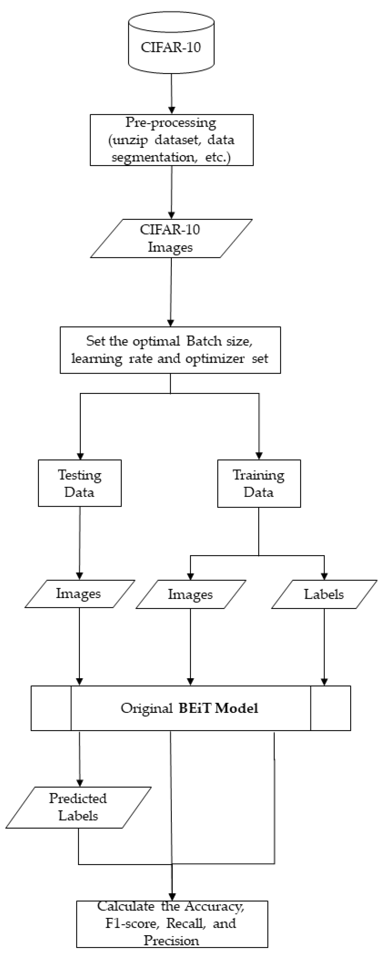
2. Materials and Methods
2.1. Pre-Training Models
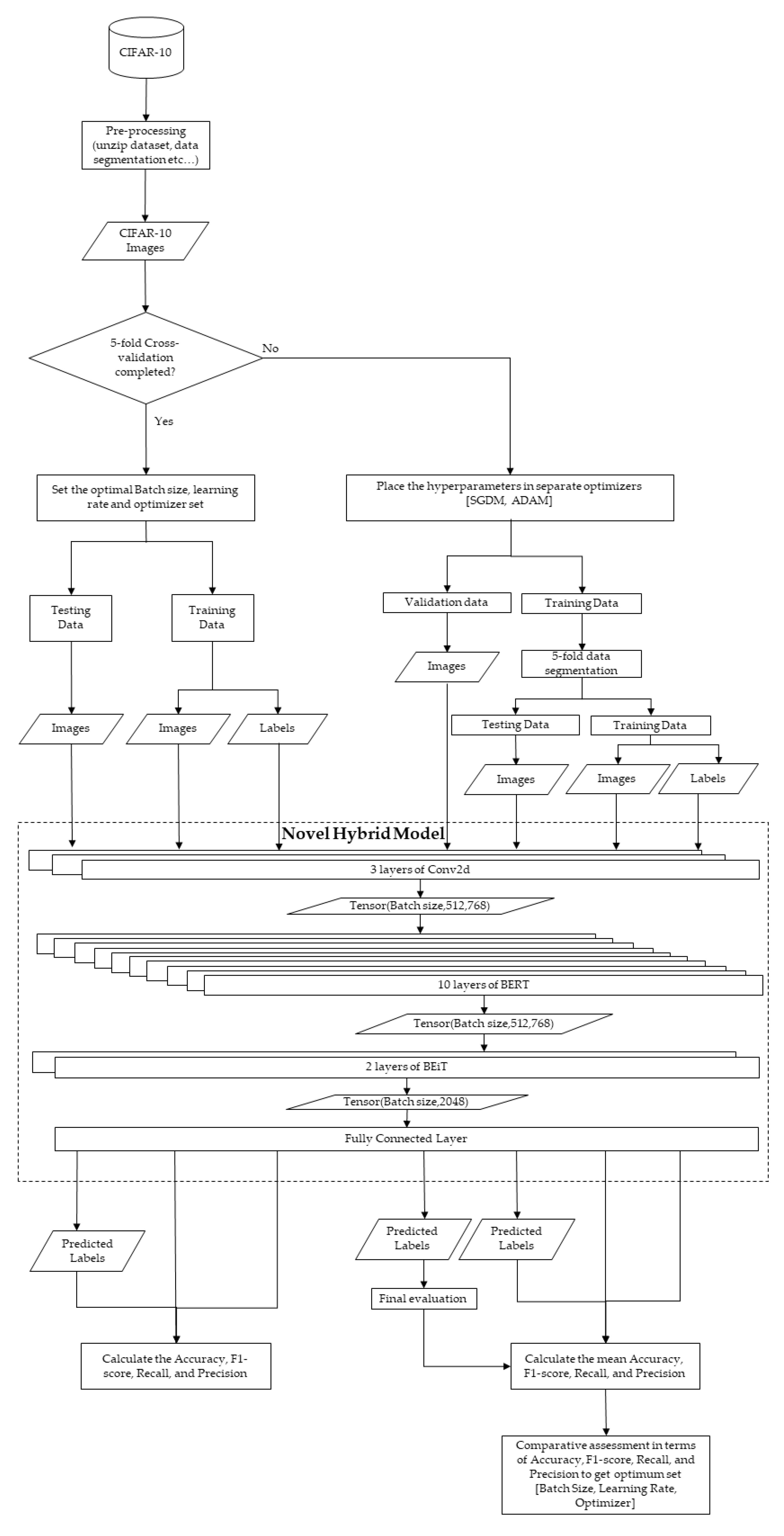
2.2. Design of a Novel Hybrid Model
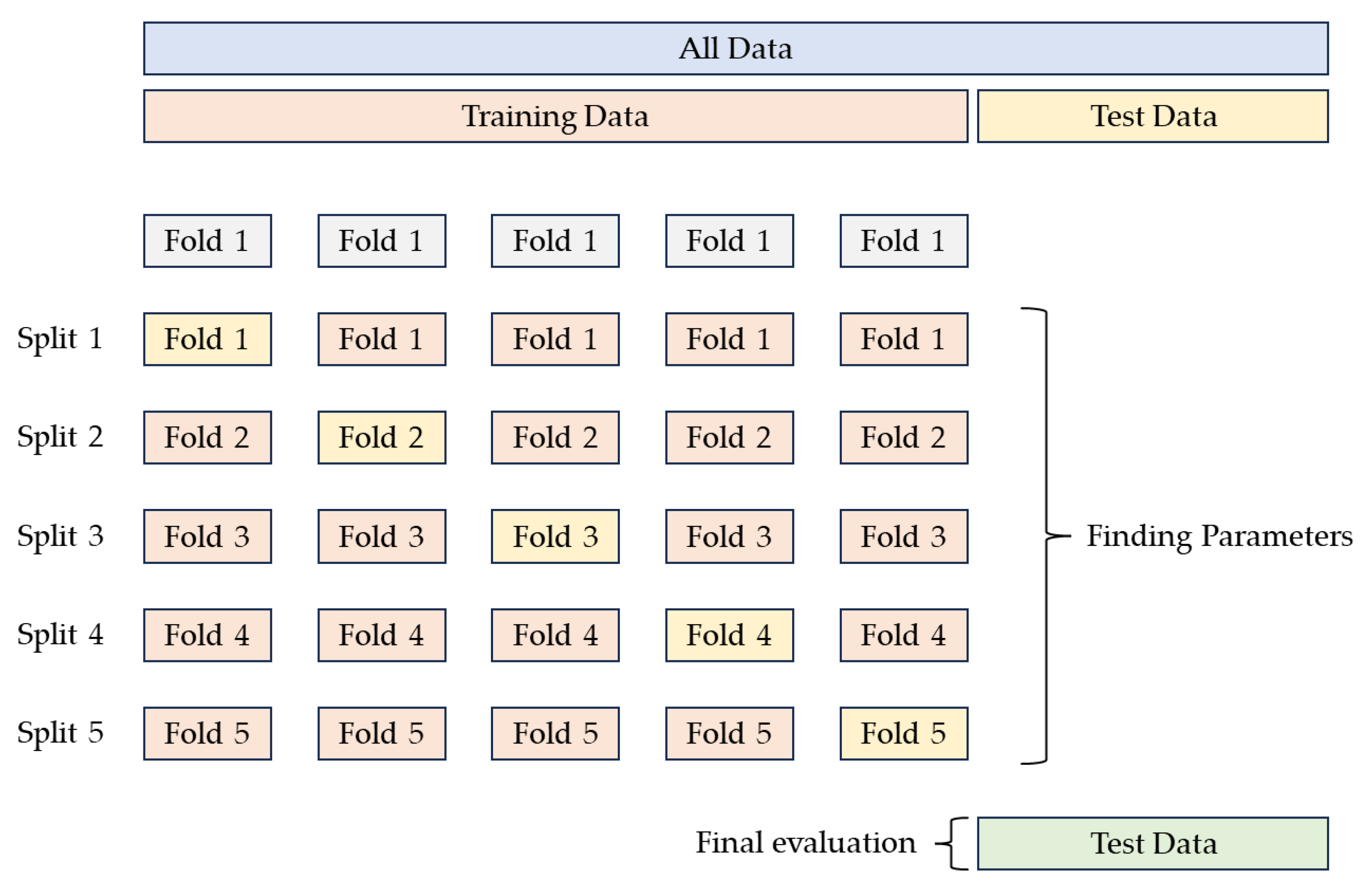
2.3. GridSearchCV and K-Fold Cross-Validation
3. Experimental Setup and Results Analysis
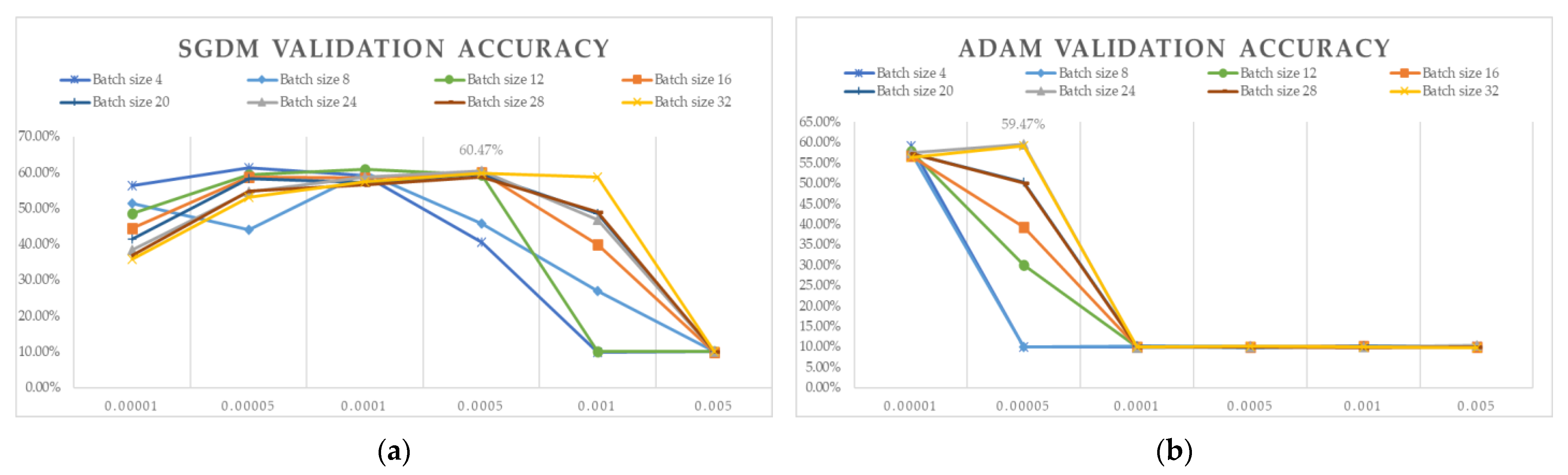
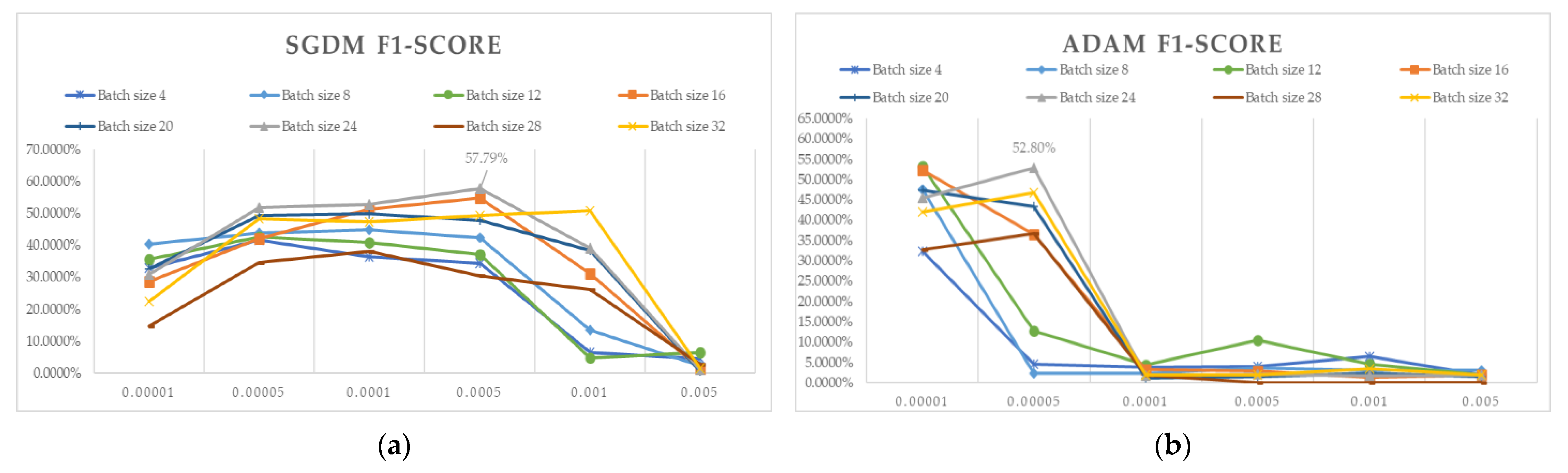
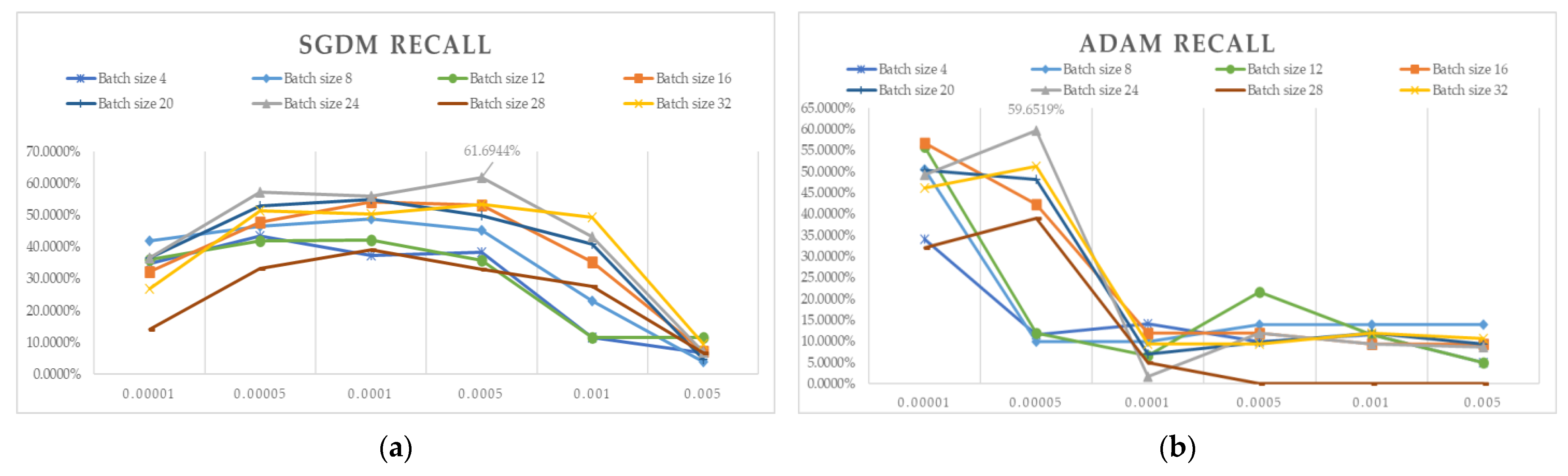
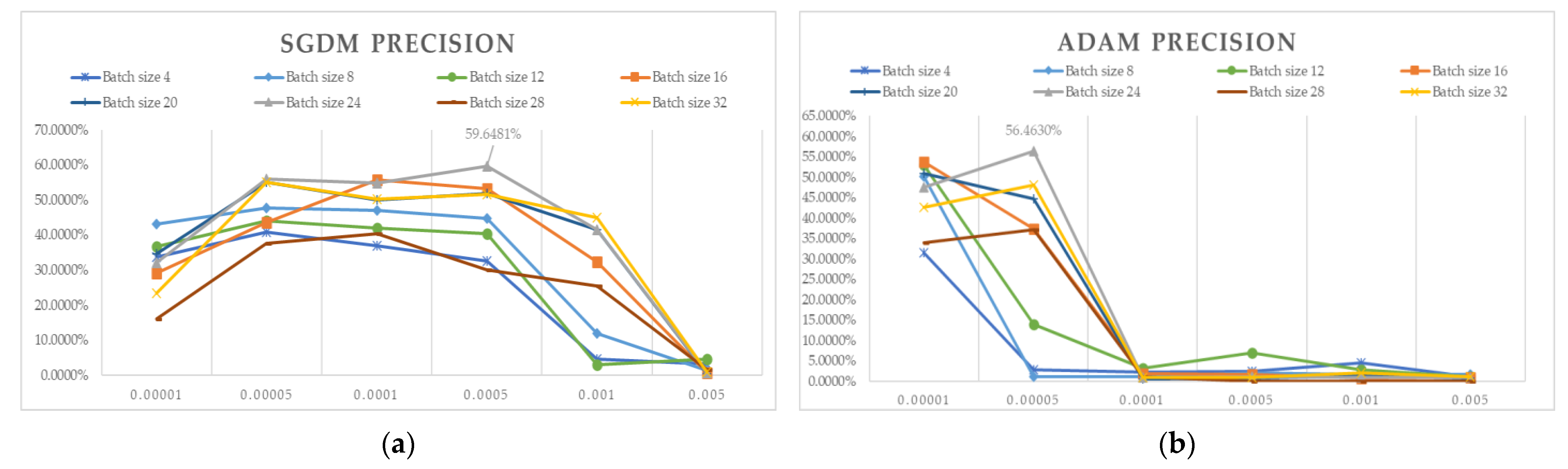
3.1. 5-Fold Cross-Validation
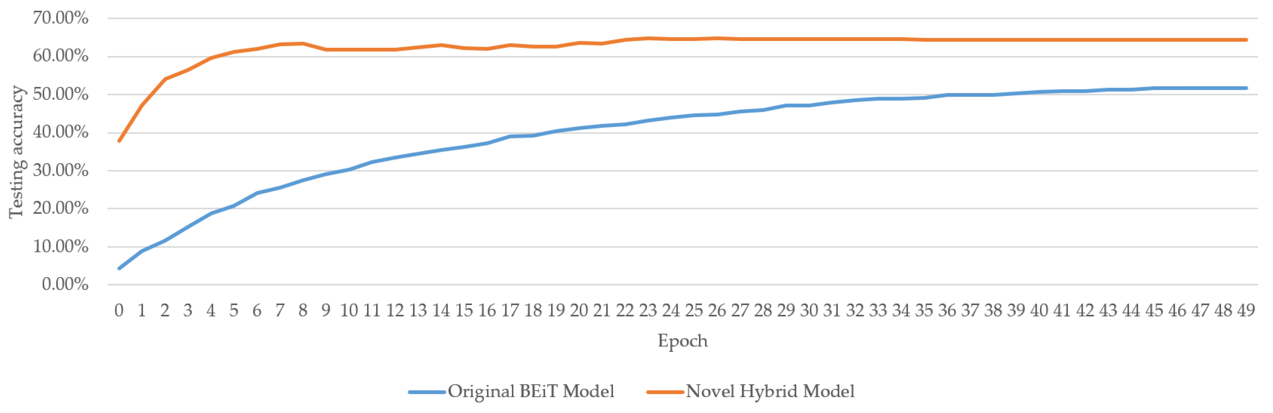
3.2. Ablation Study between the Novel Hybrid Model and Original BEiT Model
4. Conclusions and Future Works
Author Contributions
Funding
Data Availability Statement
Conflicts of Interest
Appendix A

| Layer (Type) | Output Shape | No. of Params | Layer (Type) | Output Shape | No. of Params |
|---|---|---|---|---|---|
| Conv2d-1 | [−1, 64, 32, 32] | 1792 | Linear-127 | [−1, 512, 768] | 590,592 |
| Conv2d-3 | [−1, 128, 32, 32] | 73,856 | Linear-128 | [−1, 512, 768] | 590,592 |
| Conv2d-5 | [−1, 384, 32, 32] | 442,752 | Linear-129 | [−1, 512, 768] | 590,592 |
| Linear-7 | [−1, 512, 768] | 590,592 | Linear-130 | [−1, 512, 768] | 590,592 |
| Linear-8 | [−1, 512, 768] | 590,592 | Linear-131 | [−1, 512, 768] | 590,592 |
| Linear-9 | [−1, 512, 768] | 590,592 | Linear-132 | [−1, 512, 768] | 590,592 |
| Linear-10 | [−1, 512, 768] | 590,592 | Linear-135 | [−1, 512, 768] | 590,592 |
| Linear-11 | [−1, 512, 768] | 590,592 | Linear-136 | [−1, 512, 768] | 590,592 |
| Linear-12 | [−1, 512, 768] | 590,592 | LayerNorm-139 | [−1, 512, 768] | 1536 |
| Linear-15 | [−1, 512, 768] | 590,592 | LayerNorm-140 | [−1, 512, 768] | 1536 |
| Linear-16 | [−1, 512, 768] | 590,592 | Linear-141 | [−1, 512, 3072] | 2,362,368 |
| LayerNorm-19 | [−1, 512, 768] | 1536 | Linear-142 | [−1, 512, 3072] | 2,362,368 |
| LayerNorm-20 | [−1, 512, 768] | 1536 | Linear-145 | [−1, 512, 768] | 2,360,064 |
| Linear-21 | [−1, 512, 3072] | 2,362,368 | Linear-146 | [−1, 512, 768] | 2,360,064 |
| Linear-22 | [−1, 512, 3072] | 2,362,368 | LayerNorm-149 | [−1, 512, 768] | 1536 |
| Linear-25 | [−1, 512, 768] | 2,360,064 | LayerNorm-150 | [−1, 512, 768] | 1536 |
| Linear-26 | [−1, 512, 768] | 2,360,064 | Linear-151 | [−1, 512, 768] | 590,592 |
| LayerNorm-29 | [−1, 512, 768] | 1536 | Linear-152 | [−1, 512, 768] | 590,592 |
| LayerNorm-30 | [−1, 512, 768] | 1536 | Linear-153 | [−1, 512, 768] | 590,592 |
| Linear-31 | [−1, 512, 768] | 590,592 | Linear-154 | [−1, 512, 768] | 590,592 |
| Linear-32 | [−1, 512, 768] | 590,592 | Linear-155 | [−1, 512, 768] | 590,592 |
| Linear-33 | [−1, 512, 768] | 590,592 | Linear-156 | [−1, 512, 768] | 590,592 |
| Linear-34 | [−1, 512, 768] | 590,592 | Linear-159 | [−1, 512, 768] | 590,592 |
| Linear-35 | [−1, 512, 768] | 590,592 | Linear-160 | [−1, 512, 768] | 590,592 |
| Linear-36 | [−1, 512, 768] | 590,592 | LayerNorm-163 | [−1, 512, 768] | 1536 |
| Linear-39 | [−1, 512, 768] | 590,592 | LayerNorm-164 | [−1, 512, 768] | 1536 |
| Linear-40 | [−1, 512, 768] | 590,592 | Linear-165 | [−1, 512, 3072] | 2,362,368 |
| LayerNorm-43 | [−1, 512, 768] | 1536 | Linear-166 | [−1, 512, 3072] | 2,362,368 |
| LayerNorm-44 | [−1, 512, 768] | 1536 | Linear-169 | [−1, 512, 768] | 2,360,064 |
| Linear-45 | [−1, 512, 3072] | 2,362,368 | Linear-170 | [−1, 512, 768] | 2,360,064 |
| Linear-46 | [−1, 512, 3072] | 2,362,368 | LayerNorm-173 | [−1, 512, 768] | 1536 |
| Linear-49 | [−1, 512, 768] | 2,360,064 | LayerNorm-174 | [−1, 512, 768] | 1536 |
| Linear-50 | [−1, 512, 768] | 2,360,064 | Linear-175 | [−1, 512, 768] | 590,592 |
| LayerNorm-53 | [−1, 512, 768] | 1536 | Linear-176 | [−1, 512, 768] | 590,592 |
| LayerNorm-54 | [−1, 512, 768] | 1536 | Linear-177 | [−1, 512, 768] | 590,592 |
| Linear-55 | [−1, 512, 768] | 590,592 | Linear-178 | [−1, 512, 768] | 590,592 |
| Linear-56 | [−1, 512, 768] | 590,592 | Linear-179 | [−1, 512, 768] | 590,592 |
| Linear-57 | [−1, 512, 768] | 590,592 | Linear-180 | [−1, 512, 768] | 590,592 |
| Linear-58 | [−1, 512, 768] | 590,592 | Linear-183 | [−1, 512, 768] | 590,592 |
| Linear-59 | [−1, 512, 768] | 590,592 | Linear-184 | [−1, 512, 768] | 590,592 |
| Linear-60 | [−1, 512, 768] | 590,592 | LayerNorm-187 | [−1, 512, 768] | 1536 |
| Linear-63 | [−1, 512, 768] | 590,592 | LayerNorm-188 | [−1, 512, 768] | 1536 |
| Linear-64 | [−1, 512, 768] | 590,592 | Linear-189 | [−1, 512, 3072] | 2,362,368 |
| LayerNorm-67 | [−1, 512, 768] | 1536 | Linear-190 | [−1, 512, 3072] | 2,362,368 |
| LayerNorm-68 | [−1, 512, 768] | 1536 | Linear-193 | [−1, 512, 768] | 2,360,064 |
| Linear-69 | [−1, 512, 3072] | 2,362,368 | Linear-194 | [−1, 512, 768] | 2,360,064 |
| Linear-70 | [−1, 512, 3072] | 2,362,368 | LayerNorm-197 | [−1, 512, 768] | 1536 |
| Linear-73 | [−1, 512, 768] | 2,360,064 | LayerNorm-198 | [−1, 512, 768] | 1536 |
| Linear-74 | [−1, 512, 768] | 2,360,064 | Linear-199 | [−1, 512, 768] | 590,592 |
| LayerNorm-77 | [−1, 512, 768] | 1536 | Linear-200 | [−1, 512, 768] | 590,592 |
| LayerNorm-78 | [−1, 512, 768] | 1536 | Linear-201 | [−1, 512, 768] | 590,592 |
| Linear-79 | [−1, 512, 768] | 590,592 | Linear-202 | [−1, 512, 768] | 590,592 |
| Linear-80 | [−1, 512, 768] | 590,592 | Linear-203 | [−1, 512, 768] | 590,592 |
| Linear-81 | [−1, 512, 768] | 590,592 | Linear-204 | [−1, 512, 768] | 590,592 |
| Linear-82 | [−1, 512, 768] | 590,592 | Linear-207 | [−1, 512, 768] | 590,592 |
| Linear-83 | [−1, 512, 768] | 590,592 | Linear-208 | [−1, 512, 768] | 590,592 |
| Linear-84 | [−1, 512, 768] | 590,592 | LayerNorm-211 | [−1, 512, 768] | 1536 |
| Linear-87 | [−1, 512, 768] | 590,592 | LayerNorm-212 | [−1, 512, 768] | 1536 |
| Linear-88 | [−1, 512, 768] | 590,592 | Linear-213 | [−1, 512, 3072] | 2,362,368 |
| LayerNorm-91 | [−1, 512, 768] | 1536 | Linear-214 | [−1, 512, 3072] | 2,362,368 |
| LayerNorm-92 | [−1, 512, 768] | 1536 | Linear-217 | [−1, 512, 768] | 2,360,064 |
| Linear-93 | [−1, 512, 3072] | 2,362,368 | Linear-218 | [−1, 512, 768] | 2,360,064 |
| Linear-94 | [−1, 512, 3072] | 2,362,368 | LayerNorm-221 | [−1, 512, 768] | 1536 |
| Linear-97 | [−1, 512, 768] | 2,360,064 | LayerNorm-222 | [−1, 512, 768] | 1536 |
| Linear-98 | [−1, 512, 768] | 2,360,064 | Linear-223 | [−1, 512, 768] | 590,592 |
| LayerNorm-101 | [−1, 512, 768] | 1536 | Linear-224 | [−1, 512, 768] | 590,592 |
| LayerNorm-102 | [−1, 512, 768] | 1536 | Linear-225 | [−1, 512, 768] | 590,592 |
| Linear-103 | [−1, 512, 768] | 590,592 | Linear-226 | [−1, 512, 768] | 590,592 |
| Linear-104 | [−1, 512, 768] | 590,592 | Linear-227 | [−1, 512, 768] | 590,592 |
| Linear-105 | [−1, 512, 768] | 590,592 | Linear-228 | [−1, 512, 768] | 590,592 |
| Linear-106 | [−1, 512, 768] | 590,592 | Linear-231 | [−1, 512, 768] | 590,592 |
| Linear-107 | [−1, 512, 768] | 590,592 | Linear-232 | [−1, 512, 768] | 590,592 |
| Linear-108 | [−1, 512, 768] | 590,592 | LayerNorm-235 | [−1, 512, 768] | 1536 |
| Linear-111 | [−1, 512, 768] | 590,592 | LayerNorm-236 | [−1, 512, 768] | 1536 |
| Linear-112 | [−1, 512, 768] | 590,592 | Linear-237 | [−1, 512, 3072] | 2,362,368 |
| LayerNorm-115 | [−1, 512, 768] | 1536 | Linear-238 | [−1, 512, 3072] | 2,362,368 |
| LayerNorm-116 | [−1, 512, 768] | 1536 | Linear-241 | [−1, 512, 768] | 2,360,064 |
| Linear-117 | [−1, 512, 3072] | 2,362,368 | Linear-242 | [−1, 512, 768] | 2,360,064 |
| Linear-118 | [−1, 512, 3072] | 2,362,368 | LayerNorm-245 | [−1, 512, 768] | 1536 |
| Linear-121 | [−1, 512, 768] | 2,360,064 | LayerNorm-246 | [−1, 512, 768] | 1536 |
| Linear-122 | [−1, 512, 768] | 2,360,064 | LayerNorm-247 | [−1, 197, 768] | 1536 |
| LayerNorm-125 | [−1, 512, 768] | 1536 | Linear-249 | [−1, 197, 768] | 590,592 |
| LayerNorm-126 | [−1, 512, 768] | 1536 | LayerNorm-252 | [−1, 197, 768] | 1536 |
| Total params: 152,928,522 Trainable params: 152,928,522 Non-trainable params: 0 Input size (MB): 0.011719 Forward/backward pass size (MB): 1562.278091 Params size (MB): 583.376015 Estimated Total Size (MB): 2145.665825 | Linear−253 | [−1, 197, 3072] | 2,362,368 | ||
| Linear−256 | [−1, 197, 768] | 2,360,064 | |||
| LayerNorm−259 | [−1, 197, 768] | 1536 | |||
| Linear−261 | [−1, 197, 768] | 590,592 | |||
| LayerNorm−264 | [−1, 197, 768] | 1536 | |||
| Linear−265 | [−1, 197, 3072] | 2,362,368 | |||
| Linear−268 | [−1, 197, 768] | 2,360,064 | |||
| Linear−271 | [−1, 10] | 20,490 | |||
Appendix B
| SGDM | |||||||||||||
|---|---|---|---|---|---|---|---|---|---|---|---|---|---|
| Batch Size | LR | Fold | Val Accuracy | F1-Score | Recall | Precision | Batch Size | LR | Fold | Val Accuracy | F1-Score | Recall | Precision |
| 4 | 0.00001 | 1 | 53.52% | 33.33% | 40.00% | 30.00% | 8 | 0.00001 | 1 | 49.53% | 43.33% | 45.83% | 43.75% |
| 2 | 57.86% | 33.33% | 30.00% | 40.00% | 2 | 51.91% | 61.90% | 64.29% | 64.29% | ||||
| 3 | 57.3% | 66.67% | 75.00% | 62.50% | 3 | 52.70% | 63.89% | 66.67% | 66.67% | ||||
| 4 | 55.7% | 20.00% | 20.00% | 20.00% | 4 | 51.87% | 8.33% | 6.25% | 12.50% | ||||
| 5 | 57.22% | 11.11% | 8.33% | 16.67% | 5 | 51.13% | 24.76% | 26.19% | 28.46% | ||||
| Mean | 56.32% | 32.89% | 34.67% | 33.83% | Mean | 51.43% | 40.44% | 41.85% | 43.15% | ||||
| 0.00005 | 1 | 62.00% | 33.33% | 33.33% | 33.33% | 0.00005 | 1 | 61.63% | 54.76% | 61.90% | 57.14% | ||
| 2 | 60.55% | 50.00% | 50.00% | 50.00% | 2 | 61.62% | 52.38% | 57.14% | 57.14% | ||||
| 3 | 61.33% | 66.67% | 75.00% | 62.50% | 3 | 60.74% | 74.44% | 75.00% | 77.78% | ||||
| 4 | 60.01% | 33.33% | 33.33% | 33.33% | 4 | 60.70% | 23.81% | 28.57% | 21.43% | ||||
| 5 | 62.68% | 25.00% | 25.00% | 25.00% | 5 | 61.98% | 14.58% | 10.42% | 25.00% | ||||
| Mean | 61.31% | 41.67% | 43.33% | 40.83% | Mean | 44.00% | 44.00% | 46.61% | 47.70% | ||||
| 0.0001 | 1 | 56.5% | 16.67% | 16.67% | 16.67% | 0.0001 | 1 | 61.92% | 34.26% | 33.33% | 35.71% | ||
| 2 | 59.8% | 50.00% | 50.00% | 50.00% | 2 | 61.26% | 40.48% | 42.86% | 42.86% | ||||
| 3 | 62.45% | 41.67% | 50.00% | 37.50% | 3 | 60.67% | 55.56% | 58.33% | 58.33% | ||||
| 4 | 58.63% | 60.00% | 60.00% | 60.00% | 4 | 53.09% | 28.57% | 35.71% | 31.43% | ||||
| 5 | 58.36% | 13.33% | 10.00% | 20.00% | 5 | 63.20% | 66.00% | 73.33% | 66.67% | ||||
| Mean | 59.15% | 36.33% | 37.33% | 36.83% | Mean | 60.03% | 44.98% | 48.71% | 47.00% | ||||
| 0.0005 | 1 | 61.17% | 33.33% | 33.33% | 33.33% | 0.0005 | 1 | 55.87% | 39.58% | 41.67% | 43.75% | ||
| 2 | 62.00% | 50.00% | 50.00% | 50.00% | 2 | 56.74% | 58.33% | 56.25% | 62.50% | ||||
| 3 | 10.22% | 0.00% | 0.00% | 0.00% | 3 | 47.04% | 80.00% | 83.33% | 77.78% | ||||
| 4 | 59.19% | 66.67% | 75.00% | 62.50% | 4 | 59.18% | 29.17% | 25.00% | 37.50% | ||||
| 5 | 9.88% | 22.22% | 33.33% | 16.67% | 5 | 10.06% | 4.44% | 2.00% | 2.50% | ||||
| Mean | 40.49% | 34.44% | 38.33% | 32.50% | Mean | 45.78% | 42.31% | 45.25% | 44.81% | ||||
| 0.001 | 1 | 10.2% | 0.00% | 0.00% | 0.00% | 0.001 | 1 | 9.69% | 0.00% | 0.00% | 0.00% | ||
| 2 | 9.92% | 0.00% | 0.00% | 0.00% | 2 | 45.19% | 40.48% | 50.00% | 40.48% | ||||
| 3 | 9.74% | 10.00% | 25.00% | 6.25% | 3 | 59.85% | 19.05% | 28.57% | 14.29% | ||||
| 4 | 10.01% | 0.00% | 0.00% | 0.00% | 4 | 9.98% | 3.70% | 16.67% | 2.08% | ||||
| 5 | 9.88% | 22.22% | 33.33% | 16.67% | 5 | 10.03% | 4.44% | 20.00% | 2.50% | ||||
| Mean | 9.95% | 6.44% | 11.67% | 4.58% | Mean | 26.95% | 13.53% | 23.05% | 11.87% | ||||
| 0.005 | 1 | 10.20% | 0.00% | 0.00% | 0.00% | 0.005 | 1 | 10.20% | 0.00% | 0.00% | 0.00% | ||
| 2 | 10.33% | 0.00% | 0.00% | 0.00% | 2 | 10.33% | 0.00% | 0.00% | 0.00% | ||||
| 3 | 9.91% | 0.00% | 0.00% | 0.00% | 3 | 9.91% | 0.00% | 0.00% | 0.00% | ||||
| 4 | 9.68% | 0.00% | 0.00% | 0.00% | 4 | 9.68% | 0.00% | 0.00% | 0.00% | ||||
| 5 | 9.88% | 22.22% | 33.33% | 16.67% | 5 | 10.10% | 10.91% | 20.00% | 7.50% | ||||
| Mean | 10.00% | 4.44% | 6.67% | 3.33% | Mean | 10.04% | 2.18% | 4.00% | 1.50% | ||||
| 12 | 0.00001 | 1 | 48.55% | 33.33% | 33.33% | 33.33% | 16 | 0.00001 | 1 | 44.38% | 38.52% | 43.33% | 41.67% |
| 2 | 48.11% | 66.67% | 62.50% | 75.00% | 2 | 46.77% | 46.87% | 56.25% | 45.00% | ||||
| 3 | 47.46% | 33.33% | 40.00% | 30.00% | 3 | 44.78% | 30.50% | 32.50% | 29.17% | ||||
| 4 | 49.04% | 20.00% | 20.00% | 20.00% | 4 | 43.87% | 14.00% | 15.00% | 15.83% | ||||
| 5 | 49.87% | 25.00% | 25.00% | 25.00% | 5 | 42.51% | 14.00% | 14.33% | 14.33% | ||||
| Mean | 48.60% | 35.67% | 36.17% | 36.67% | Mean | 44.46% | 28.78% | 32.28% | 29.20% | ||||
| 0.00005 | 1 | 57.77% | 60.00% | 60.00% | 60.00% | 0.00005 | 1 | 58.00% | 41.48% | 48.89% | 43.52% | ||
| 2 | 61.49% | 100.00% | 100.00% | 100.00% | 2 | 61.71% | 66.93% | 66.67% | 69.44% | ||||
| 3 | 59.22% | 20.00% | 20.00% | 20.00% | 3 | 58.89% | 31.69% | 44.44% | 26.30% | ||||
| 4 | 59.59% | 20.00% | 20.00% | 20.00% | 4 | 57.47% | 27.67% | 37.50% | 29.17% | ||||
| 5 | 58.08% | 13.33% | 10.00% | 20.00% | 5 | 57.58% | 43.15% | 41.85% | 50.00% | ||||
| Mean | 59.23% | 42.67% | 42.00% | 44.00% | Mean | 58.73% | 42.18% | 47.87% | 43.69% | ||||
| 0.0001 | 1 | 61.68% | 14.29% | 14.29% | 14.29% | 0.0001 | 1 | 57.37% | 55.37% | 62.22% | 53.70% | ||
| 2 | 62.67% | 66.67% | 62.50% | 75.00% | 2 | 63.05% | 59.26% | 57.41% | 62.96% | ||||
| 3 | 58.44% | 33.33% | 40.00% | 30.00% | 3 | 61.01% | 49.01% | 56.48% | 53.17% | ||||
| 4 | 62.01% | 65.21% | 68.75% | 65.83% | 4 | 61.52% | 45.00% | 42.50% | 50.00% | ||||
| 5 | 59.87% | 25.00% | 25.00% | 25.00% | 5 | 59.38% | 47.83% | 52.59% | 58.33% | ||||
| Mean | 60.93% | 40.90% | 42.11% | 42.02% | Mean | 60.47% | 51.29% | 54.24% | 55.63% | ||||
| 0.0005 | 1 | 59.34% | 33.33% | 33.33% | 33.33% | 0.0005 | 1 | 63.73% | 61.46% | 70.00% | 63.54% | ||
| 2 | 58.71% | 33.33% | 33.33% | 33.33% | 2 | 60.60% | 41.67% | 50.00% | 37.50% | ||||
| 3 | 59.36% | 45.67% | 42.50% | 55.00% | 3 | 57.44% | 48.89% | 52.78% | 46.76% | ||||
| 4 | 60.51% | 40.00% | 40.00% | 40.00% | 4 | 58.33% | 45.67% | 42.50% | 55.00% | ||||
| 5 | 58.44% | 33.33% | 30.00% | 40.00% | 5 | 60.22% | 54.50% | 50.74% | 62.96% | ||||
| Mean | 59.27% | 37.13% | 35.83% | 40.33% | Mean | 60.06% | 50.44% | 53.20% | 53.15% | ||||
| 0.001 | 1 | 10.11% | 10.00% | 25.00% | 6.25% | 0.001 | 1 | 10.01% | 5.95% | 12.50% | 3.91% | ||
| 2 | 10.14% | 0.00% | 0.00% | 0.00% | 2 | 58.75% | 70.42% | 70.83% | 72.92% | ||||
| 3 | 10.00% | 0.00% | 0.00% | 0.00% | 3 | 59.32% | 34.05% | 45.00% | 30.00% | ||||
| 4 | 9.73% | 0.00% | 0.00% | 0.00% | 4 | 60.89% | 45.33% | 47.50% | 55.00% | ||||
| 5 | 10.06% | 13.33% | 33.33% | 8.33% | 5 | 10.24% | 0.00% | 0.00% | 0.00% | ||||
| Mean | 10.01% | 4.67% | 11.67% | 2.92% | Mean | 39.84% | 31.15% | 35.17% | 32.36% | ||||
| 0.005 | 1 | 10.20% | 0.00% | 0.00% | 0.00% | 0.005 | 1 | 10.20% | 0.00% | 0.00% | 0.00% | ||
| 2 | 10.33% | 0.00% | 0.00% | 0.00% | 2 | 9.92% | 2.78% | 12.50% | 1.56% | ||||
| 3 | 9.91% | 0.00% | 0.00% | 0.00% | 3 | 9.91% | 1.31% | 11.11% | 0.69% | ||||
| 4 | 9.98% | 10.00% | 25.00% | 6.25% | 4 | 9.68% | 0.00% | 0.00% | 0.00% | ||||
| 5 | 9.88% | 22.22% | 33.33% | 16.67% | 5 | 9.88% | 2.78% | 12.50% | 1.56% | ||||
| Mean | 10.06% | 6.44% | 11.67% | 4.58% | Mean | 9.92% | 1.37% | 7.22% | 0.76% | ||||
| 20 | 0.00001 | 1 | 42.66% | 35.19% | 41.85% | 33.33% | 24 | 0.00001 | 1 | 40.49% | 32.08% | 43.75% | 31.67% |
| 2 | 42.15% | 59.26% | 65.63% | 62.50% | 2 | 38.41% | 52.28% | 51.85% | 60.00% | ||||
| 3 | 40.08% | 31.33% | 37.50% | 29.17% | 3 | 38.54% | 22.52% | 32.50% | 18.33% | ||||
| 4 | 41.68% | 19.60% | 19.76% | 29.00% | 4 | 37.56% | 18.33% | 25.00% | 18.33% | ||||
| 5 | 40.76% | 17.46% | 18.15% | 19.75% | 5 | 36.32% | 29.63% | 29.26% | 32.28% | ||||
| Mean | 41.47% | 32.57% | 36.58% | 34.75% | Mean | 38.26% | 30.97% | 36.47% | 32.12% | ||||
| 0.00005 | 1 | 56.44% | 58.81% | 65.83% | 58.33% | 0.00005 | 1 | 55.67% | 44.81% | 57.78% | 49.07% | ||
| 2 | 59.93% | 67.10% | 71.88% | 76.88% | 2 | 52.94% | 63.81% | 64.58% | 71.67% | ||||
| 3 | 58.99% | 44.36% | 47.50% | 44.33% | 3 | 54.86% | 52.65% | 58.33% | 50.37% | ||||
| 4 | 57.21% | 31.67% | 32.62% | 38.33% | 4 | 56.01% | 28.00% | 32.50% | 33.33% | ||||
| 5 | 58.30% | 45.17% | 46.17% | 57.50% | 5 | 53.71% | 69.71% | 73.33% | 75.00% | ||||
| Mean | 58.17% | 49.42% | 52.80% | 55.08% | Mean | 54.64% | 51.80% | 57.31% | 55.89% | ||||
| 0.0001 | 1 | 60.15% | 56.16% | 60.00% | 60.37% | 0.0001 | 1 | 59.66% | 45.33% | 51.00% | 42.50% | ||
| 2 | 62.88% | 63.65% | 66.67% | 62.04% | 2 | 58.20% | 67.56% | 68.75% | 73.75% | ||||
| 3 | 59.50% | 47.35% | 51.85% | 44.44% | 3 | 60.64% | 38.70% | 47.22% | 34.26% | ||||
| 4 | 61.04% | 37.12% | 40.95% | 39.17% | 4 | 58.66% | 52.00% | 52.50% | 56.67% | ||||
| 5 | 62.16% | 44.71% | 55.74% | 44.44% | 5 | 56.70% | 60.74% | 60.74% | 67.46% | ||||
| Mean | 61.15% | 49.80% | 55.04% | 50.09% | Mean | 58.77% | 52.87% | 56.04% | 54.93% | ||||
| 0.0005 | 1 | 57.81% | 53.41% | 56.67% | 55.56% | 0.0005 | 1 | 59.01% | 53.39% | 60.00% | 53.70% | ||
| 2 | 58.31% | 54.29% | 55.00% | 59.17% | 2 | 62.81% | 65.21% | 68.75% | 65.83% | ||||
| 3 | 63.36% | 57.17% | 60.00% | 61.00% | 3 | 62.92% | 67.65% | 72.22% | 64.44% | ||||
| 4 | 59.04% | 37.00% | 35.95% | 41.67% | 4 | 56.93% | 37.00% | 37.50% | 46.67% | ||||
| 5 | 58.73% | 37.38% | 41.83% | 41.50% | 5 | 60.70% | 65.70% | 70.00% | 67.59% | ||||
| Mean | 59.45% | 47.85% | 49.89% | 51.78% | Mean | 60.47% | 57.79% | 61.69% | 59.65% | ||||
| 0.001 | 1 | 57.07% | 37.08% | 42.50% | 35.42% | 0.001 | 1 | 59.05% | 53.70% | 56.67% | 58.33% | ||
| 2 | 58.38% | 61.57% | 60.00% | 69.17% | 2 | 61.08% | 57.78% | 57.41% | 62.96% | ||||
| 3 | 9.86% | 2.02% | 11.11% | 1.11% | 3 | 9.86% | 1.31% | 11.11% | 0.69% | ||||
| 4 | 59.46% | 40.33% | 40.95% | 46.67% | 4 | 46.66% | 38.89% | 41.67% | 38.89% | ||||
| 5 | 57.43% | 50.56% | 50.19% | 55.56% | 5 | 57.11% | 44.67% | 49.00% | 46.50% | ||||
| Mean | 48.44% | 38.31% | 40.95% | 41.58% | Mean | 46.75% | 39.27% | 43.17% | 41.48% | ||||
| 0.005 | 1 | 9.73% | 2.27% | 12.50% | 1.25% | 0.005 | 1 | 10.20% | 0.00% | 0.00% | 0.00% | ||
| 2 | 10.46% | 0.00% | 0.00% | 0.00% | 2 | 9.93% | 2.78% | 12.50% | 1.56% | ||||
| 3 | 9.91% | 1.06% | 11.11% | 0.56% | 3 | 9.86% | 1.31% | 11.11% | 0.69% | ||||
| 4 | 9.68% | 0.00% | 0.00% | 0.00% | 4 | 10.23% | 1.31% | 11.11% | 0.69% | ||||
| 5 | 10.24% | 0.00% | 0.00% | 0.00% | 5 | 10.24% | 0.00% | 0.00% | 0.00% | ||||
| Mean | 10.00% | 0.67% | 4.72% | 0.36% | Mean | 10.09% | 1.08% | 6.94% | 0.59% | ||||
| 28 | 0.00001 | 1 | 31.34% | 0.00% | 0.00% | 0.00% | 32 | 0.00001 | 1 | 36.77% | 21.11% | 32.22% | 23.52% |
| 2 | 37.39% | 0.00% | 0.00% | 0.00% | 2 | 39.12% | 31.10% | 37.50% | 31.25% | ||||
| 3 | 38.16% | 40.00% | 40.00% | 40.00% | 3 | 34.83% | 27.46% | 33.33% | 24.81% | ||||
| 4 | 39.94% | 20.00% | 20.00% | 20.00% | 4 | 34.98% | 15.67% | 15.00% | 18.33% | ||||
| 5 | 37.20% | 13.33% | 10.00% | 20.00% | 5 | 33.69% | 16.67% | 15.93% | 19.58% | ||||
| Mean | 36.81% | 14.67% | 14.00% | 16.00% | Mean | 35.88% | 22.40% | 26.80% | 23.50% | ||||
| 0.00005 | 1 | 56.21% | 33.33% | 33.33% | 33.33% | 0.00005 | 1 | 52.80% | 55.24% | 60.00% | 66.67% | ||
| 2 | 53.35% | 66.67% | 62.50% | 75.00% | 2 | 52.40% | 62.14% | 62.50% | 71.67% | ||||
| 3 | 54.51% | 20.00% | 20.00% | 20.00% | 3 | 53.83% | 39.52% | 47.50% | 35.83% | ||||
| 4 | 54.93% | 40.00% | 40.00% | 40.00% | 4 | 51.65% | 43.33% | 42.50% | 55.00% | ||||
| 5 | 54.70% | 13.33% | 10.00% | 20.00% | 5 | 54.21% | 41.00% | 44.33% | 46.00% | ||||
| Mean | 54.74% | 34.67% | 33.17% | 37.67% | Mean | 52.98% | 48.25% | 51.37% | 55.03% | ||||
| 0.0001 | 1 | 61.51% | 33.33% | 33.33% | 33.33% | 0.0001 | 1 | 56.69% | 57.22% | 62.22% | 59.26% | ||
| 2 | 59.69% | 66.67% | 62.50% | 75.00% | 2 | 58.72% | 72.92% | 75.00% | 75.00% | ||||
| 3 | 60.92% | 40.00% | 40.00% | 40.00% | 3 | 57.91% | 29.10% | 41.67% | 23.15% | ||||
| 4 | 58.24% | 37.50% | 50.00% | 33.33% | 4 | 55.45% | 52.00% | 47.50% | 66.67% | ||||
| 5 | 61.90% | 13.33% | 10.00% | 20.00% | 5 | 58.58% | 26.19% | 25.33% | 35.00% | ||||
| Mean | 60.45% | 38.17% | 39.17% | 40.33% | Mean | 57.47% | 47.49% | 50.34% | 50.34% | ||||
| 0.0005 | 1 | 56.86% | 16.67% | 16.67% | 16.67% | 0.0005 | 1 | 59.85% | 58.20% | 60.00% | 63.89% | ||
| 2 | 61.44% | 50.00% | 50.00% | 50.00% | 2 | 60.23% | 57.30% | 61.11% | 54.63% | ||||
| 3 | 63.29% | 41.67% | 50.00% | 37.50% | 3 | 59.80% | 44.71% | 50.00% | 42.96% | ||||
| 4 | 61.54% | 33.33% | 40.00% | 30.00% | 4 | 59.51% | 46.67% | 52.50% | 48.33% | ||||
| 5 | 60.50% | 11.11% | 8.33% | 16.67% | 5 | 59.82% | 39.52% | 43.67% | 48.33% | ||||
| Mean | 60.73% | 30.56% | 33.00% | 30.17% | Mean | 59.84% | 49.28% | 53.46% | 51.63% | ||||
| 0.001 | 1 | 58.72% | 14.29% | 14.29% | 14.29% | 0.001 | 1 | 60.31% | 36.67% | 42.22% | 34.81% | ||
| 2 | 59.69% | 50.00% | 50.00% | 50.00% | 2 | 60.94% | 37.50% | 50.00% | 33.33% | ||||
| 3 | 58.04% | 33.33% | 40.00% | 30.00% | 3 | 58.44% | 39.00% | 43.33% | 40.00% | ||||
| 4 | 58.68% | 33.33% | 33.33% | 33.33% | 4 | 56.43% | 40.33% | 42.50% | 46.67% | ||||
| 5 | 10.10% | 0.00% | 0.00% | 0.00% | 5 | 57.29% | 66.30% | 68.15% | 70.00% | ||||
| Mean | 49.05% | 26.19% | 27.52% | 25.52% | Mean | 58.68% | 43.96% | 49.24% | 44.96% | ||||
| 0.005 | 1 | 10.20% | 0.00% | 0.00% | 0.00% | 0.005 | 1 | 10.20% | 0.00% | 0.00% | 0.00% | ||
| 2 | 9.70% | 13.33% | 33.33% | 8.33% | 2 | 9.70% | 2.78% | 12.50% | 1.56% | ||||
| 3 | 9.91% | 0.00% | 0.00% | 0.00% | 3 | 9.91% | 1.31% | 11.11% | 0.69% | ||||
| 4 | 10.17% | 0.00% | 0.00% | 0.00% | 4 | 10.01% | 1.31% | 11.11% | 0.69% | ||||
| 5 | 10.10% | 0.00% | 0.00% | 0.00% | 5 | 10.06% | 2.78% | 12.50% | 1.56% | ||||
| Mean | 10.02% | 2.67% | 6.67% | 1.67% | Mean | 9.98% | 1.63% | 9.44% | 0.90% | ||||
| ADAM | |||||||||||||
| Batch size | LR | Fold | Val Accuracy | F1-score | Recall | Precision | Batch size | LR | Fold | Val Accuracy | F1-score | Recall | Precision |
| 4 | 0.00001 | 1 | 58.63% | 40.00% | 40.00% | 40.00% | 8 | 0.00001 | 1 | 56.96% | 63.81% | 66.67% | 64.29% |
| 2 | 65.19% | 20.00% | 20.00% | 20.00% | 2 | 57.84% | 45.83% | 43.75% | 50.00% | ||||
| 3 | 57.11% | 41.67% | 50.00% | 37.50% | 3 | 57.31% | 40.00% | 42.86% | 38.10% | ||||
| 4 | 57.33% | 40.00% | 40.00% | 40.00% | 4 | 57.54% | 29.52% | 35.71% | 32.14% | ||||
| 5 | 57.64% | 20.00% | 20.00% | 20.00% | 5 | 57.80% | 58.33% | 63.89% | 66.67% | ||||
| Mean | 59.18% | 32.33% | 34.00% | 31.50% | Mean | 57.49% | 47.50% | 50.58% | 50.24% | ||||
| 0.00005 | 1 | 9.73% | 0.00% | 0.00% | 0.00% | 0.00005 | 1 | 10.20% | 0.00% | 0.00% | 0.00% | ||
| 2 | 10.17% | 13.33% | 33.33% | 8.33% | 2 | 10.14% | 3.70% | 16.67% | 2.08% | ||||
| 3 | 10.25% | 10.00% | 25.00% | 6.25% | 3 | 10.25% | 3.70% | 16.67% | 2.08% | ||||
| 4 | 9.68% | 0.00% | 0.00% | 0.00% | 4 | 9.73% | 3.70% | 16.67% | 2.08% | ||||
| 5 | 10.03% | 0.00% | 0.00% | 0.00% | 5 | 9.46% | 0.00% | 0.00% | 0.00% | ||||
| Mean | 9.97% | 4.67% | 11.67% | 2.92% | Mean | 9.96% | 2.22% | 10.00% | 1.25% | ||||
| 0.0001 | 1 | 9.94% | 10.00% | 25.00% | 6.25% | 0.0001 | 1 | 10.20% | 0.00% | 0.00% | 0.00% | ||
| 2 | 10.17% | 3.70% | 16.67% | 2.08% | 2 | 9.93% | 3.70% | 16.67% | 2.08% | ||||
| 3 | 9.73% | 3.70% | 16.67% | 2.08% | 3 | 10.25% | 3.70% | 16.67% | 2.08% | ||||
| 4 | 9.46% | 1.47% | 12.50% | 0.78% | 4 | 10.40% | 3.70% | 16.67% | 2.08% | ||||
| 5 | 10.24% | 0.00% | 0.00% | 0.00% | 5 | 9.46% | 0.00% | 0.00% | 0.00% | ||||
| Mean | 9.91% | 3.77% | 14.17% | 2.24% | Mean | 10.05% | 2.22% | 10.00% | 1.25% | ||||
| 0.0005 | 1 | 9.94% | 10.00% | 25.00% | 6.25% | 0.0005 | 1 | 10.37% | 3.70% | 16.67% | 2.08% | ||
| 2 | 9.92% | 0.00% | 0.00% | 0.00% | 2 | 9.70% | 6.67% | 16.67% | 4.17% | ||||
| 3 | 10.03% | 0.00% | 0.00% | 0.00% | 3 | 10.22% | 0.00% | 0.00% | 0.00% | ||||
| 4 | 10.40% | 10.00% | 25.00% | 6.25% | 4 | 10.40% | 3.70% | 16.67% | 2.08% | ||||
| 5 | 9.46% | 0.00% | 0.00% | 0.00% | 5 | 10.06% | 4.44% | 20.00% | 2.50% | ||||
| Mean | 9.95% | 4.00% | 10.00% | 2.50% | Mean | 10.15% | 3.70% | 14.00% | 2.17% | ||||
| 0.001 | 1 | 10.37% | 10.00% | 25.00% | 6.25% | 0.001 | 1 | 9.72% | 3.70% | 16.67% | 2.08% | ||
| 2 | 9.60% | 22.22% | 33.33% | 16.67% | 2 | 10.46% | 0.00% | 0.00% | 0.00% | ||||
| 3 | 9.86% | 0.00% | 0.00% | 0.00% | 3 | 9.86% | 3.70% | 16.67% | 2.08% | ||||
| 4 | 10.44% | 0.00% | 0.00% | 0.00% | 4 | 9.73% | 3.70% | 16.67% | 2.08% | ||||
| 5 | 9.46% | 0.00% | 0.00% | 0.00% | 5 | 10.03% | 4.44% | 20.00% | 2.50% | ||||
| Mean | 9.95% | 6.44% | 11.67% | 4.58% | Mean | 9.96% | 3.11% | 14.00% | 1.75% | ||||
| 0.005 | 1 | 10.03% | 0.00% | 0.00% | 0.00% | 0.005 | 1 | 10.11% | 3.70% | 16.67% | 2.08% | ||
| 2 | 10.14% | 0.00% | 0.00% | 0.00% | 2 | 10.33% | 0.00% | 0.00% | 0.00% | ||||
| 3 | 10.22% | 0.00% | 0.00% | 0.00% | 3 | 9.86% | 3.70% | 16.67% | 2.08% | ||||
| 4 | 10.40% | 10.00% | 25.00% | 6.25% | 4 | 9.73% | 3.70% | 16.67% | 2.08% | ||||
| 5 | 9.79% | 0.00% | 0.00% | 0.00% | 5 | 10.10% | 4.44% | 20.00% | 2.50% | ||||
| Mean | 10.12% | 2.00% | 5.00% | 1.25% | Mean | 10.03% | 3.11% | 14.00% | 1.75% | ||||
| 12 | 0.00001 | 1 | 57.81% | 33.33% | 33.33% | 33.33% | 16 | 0.00001 | 1 | 56.61% | 58.33% | 62.22% | 64.81% |
| 2 | 57.96% | 100.00% | 100.00% | 100.00% | 2 | 56.60% | 66.55% | 68.75% | 67.71% | ||||
| 3 | 59.22% | 33.33% | 40.00% | 30.00% | 3 | 56.23% | 50.51% | 50.44% | 50.67% | ||||
| 4 | 56.18% | 60.00% | 60.00% | 60.00% | 4 | 57.70% | 41.00% | 45.00% | 38.33% | ||||
| 5 | 57.68% | 39.83% | 46.00% | 41.67% | 5 | 56.55% | 45.19% | 57.78% | 47.22% | ||||
| Mean | 57.77% | 53.30% | 55.87% | 53.00% | Mean | 56.74% | 52.31% | 56.84% | 53.75% | ||||
| 0.00005 | 1 | 9.73% | 0.00% | 0.00% | 0.00% | 0.00005 | 1 | 60.28% | 41.00% | 46.00% | 41.00% | ||
| 2 | 9.82% | 0.00% | 0.00% | 0.00% | 2 | 59.55% | 70.71% | 75.00% | 73.96% | ||||
| 3 | 10.00% | 0.00% | 0.00% | 0.00% | 3 | 57.40% | 65.33% | 66.67% | 68.33% | ||||
| 4 | 58.26% | 50.00% | 50.00% | 50.00% | 4 | 9.44% | 4.44% | 11.11% | 2.78% | ||||
| 5 | 61.87% | 13.33% | 10.00% | 20.00% | 5 | 9.46% | 1.47% | 12.50% | 0.78% | ||||
| Mean | 29.94% | 12.67% | 12.00% | 14.00% | Mean | 39.23% | 36.59% | 42.26% | 37.37% | ||||
| 0.0001 | 1 | 10.20% | 0.00% | 0.00% | 0.00% | 0.0001 | 1 | 9.94% | 2.78% | 12.50% | 1.56% | ||
| 2 | 9.60% | 22.22% | 33.33% | 16.67% | 2 | 9.82% | 2.78% | 12.50% | 1.56% | ||||
| 3 | 10.03% | 0.00% | 0.00% | 0.00% | 3 | 10.25% | 3.51% | 11.11% | 2.08% | ||||
| 4 | 9.73% | 0.00% | 0.00% | 0.00% | 4 | 9.44% | 4.44% | 11.11% | 2.78% | ||||
| 5 | 10.41% | 0.00% | 0.00% | 0.00% | 5 | 9.88% | 2.78% | 12.50% | 1.56% | ||||
| Mean | 9.99% | 4.44% | 6.67% | 3.33% | Mean | 9.87% | 3.26% | 11.94% | 1.91% | ||||
| 0.0005 | 1 | 10.11% | 10.00% | 25.00% | 6.25% | 0.0005 | 1 | 10.01% | 5.95% | 12.50% | 3.91% | ||
| 2 | 9.93% | 0.00% | 0.00% | 0.00% | 2 | 9.82% | 2.78% | 12.50% | 1.56% | ||||
| 3 | 9.74% | 10.00% | 25.00% | 6.25% | 3 | 9.91% | 1.31% | 11.11% | 0.69% | ||||
| 4 | 9.98% | 10.00% | 25.00% | 6.25% | 4 | 9.73% | 2.47% | 11.11% | 1.39% | ||||
| 5 | 9.88% | 22.22% | 33.33% | 16.67% | 5 | 9.93% | 1.47% | 12.50% | 0.78% | ||||
| Mean | 9.93% | 10.44% | 21.67% | 7.08% | Mean | 9.88% | 2.80% | 11.94% | 1.67% | ||||
| 0.001 | 1 | 10.20% | 0.00% | 0.00% | 0.00% | 0.001 | 1 | 10.20% | 1.47% | 12.50% | 0.78% | ||
| 2 | 9.93% | 0.00% | 0.00% | 0.00% | 2 | 9.92% | 2.78% | 12.50% | 1.56% | ||||
| 3 | 9.86% | 0.00% | 0.00% | 0.00% | 3 | 9.86% | 1.31% | 11.11% | 0.69% | ||||
| 4 | 10.40% | 10.00% | 25.00% | 6.25% | 4 | 10.17% | 1.31% | 11.11% | 0.69% | ||||
| 5 | 10.06% | 13.33% | 33.33% | 8.33% | 5 | 10.41% | 0.00% | 0.00% | 0.00% | ||||
| Mean | 10.09% | 4.67% | 11.67% | 2.92% | Mean | 10.11% | 1.37% | 9.44% | 0.75% | ||||
| 0.005 | 1 | 10.37% | 10.00% | 25.00% | 6.25% | 0.005 | 1 | 9.94% | 2.78% | 12.50% | 1.56% | ||
| 2 | 10.14% | 0.00% | 0.00% | 0.00% | 2 | 9.92% | 2.78% | 12.50% | 1.56% | ||||
| 3 | 9.91% | 0.00% | 0.00% | 0.00% | 3 | 9.96% | 1.31% | 11.11% | 0.69% | ||||
| 4 | 9.73% | 0.00% | 0.00% | 0.00% | 4 | 9.82% | 0.00% | 0.00% | 0.00% | ||||
| 5 | 9.93% | 0.00% | 0.00% | 0.00% | 5 | 9.95% | 1.47% | 12.50% | 0.78% | ||||
| Mean | 10.02% | 2.00% | 5.00% | 1.25% | Mean | 9.87% | 1.99% | 9.41% | 0.91% | ||||
| 20 | 0.00001 | 1 | 57.32% | 68.81% | 69.58% | 80.21% | 24 | 0.00001 | 1 | 57.68% | 39.83% | 46.00% | 41.67% |
| 2 | 59.61% | 62.78% | 62.96% | 63.89% | 2 | 57.35% | 45.93% | 50.00% | 46.30% | ||||
| 3 | 56.62% | 61.48% | 69.44% | 59.26% | 3 | 57.34% | 43.46% | 48.15% | 41.48% | ||||
| 4 | 56.34% | 41.94% | 37.38% | 50.00% | 4 | 56.63% | 28.00% | 30.00% | 31.67% | ||||
| 5 | 57.02% | 2.27% | 12.50% | 1.25% | 5 | 58.08% | 69.74% | 72.50% | 76.04% | ||||
| Mean | 57.38% | 47.46% | 50.37% | 50.92% | Mean | 57.42% | 45.39% | 49.33% | 47.43% | ||||
| 0.00005 | 1 | 60.15% | 48.24% | 49.00% | 60.33% | 0.00005 | 1 | 60.55% | 63.54% | 70.00% | 66.67% | ||
| 2 | 61.36% | 70.63% | 71.13% | 70.33% | 2 | 60.09% | 49.63% | 51.85% | 48.15% | ||||
| 3 | 59.93% | 42.95% | 53.33% | 38.17% | 3 | 59.16% | 68.52% | 76.85% | 72.22% | ||||
| 4 | 60.65% | 52.59% | 56.61% | 53.70% | 4 | 58.80% | 39.26% | 47.22% | 44.44% | ||||
| 5 | 9.79% | 2.47% | 11.11% | 1.39% | 5 | 58.76% | 43.05% | 52.33% | 50.83% | ||||
| Mean | 50.38% | 43.38% | 48.24% | 44.79% | Mean | 59.47% | 52.80% | 59.65% | 56.46% | ||||
| 0.0001 | 1 | 9.72% | 2.27% | 12.50% | 1.25% | 0.0001 | 1 | 9.72% | 1.47% | 12.50% | 0.78% | ||
| 2 | 10.33% | 0.00% | 0.00% | 0.00% | 2 | 9.82% | 2.78% | 12.50% | 1.56% | ||||
| 3 | 9.86% | 2.02% | 11.11% | 1.11% | 3 | 9.74% | 2.47% | 11.11% | 1.39% | ||||
| 4 | 10.23% | 1.06% | 11.11% | 0.56% | 4 | 9.68% | 0.00% | 0.00% | 0.00% | ||||
| 5 | 10.24% | 0.00% | 0.00% | 0.00% | 5 | 9.46% | 1.47% | 12.50% | 0.78% | ||||
| Mean | 10.08% | 1.07% | 6.94% | 0.58% | Mean | 9.68% | 1.64% | 1.64% | 0.90% | ||||
| 0.0005 | 1 | 9.72% | 2.27% | 12.50% | 1.25% | 0.0005 | 1 | 10.37% | 2.78% | 12.50% | 1.56% | ||
| 2 | 9.70% | 2.27% | 12.50% | 1.25% | 2 | 9.92% | 2.78% | 12.50% | 1.56% | ||||
| 3 | 9.91% | 1.06% | 11.11% | 0.56% | 3 | 10.22% | 1.31% | 11.11% | 0.69% | ||||
| 4 | 9.68% | 0.00% | 0.00% | 0.00% | 4 | 9.73% | 2.47% | 11.11% | 1.39% | ||||
| 5 | 9.79% | 2.27% | 12.50% | 1.25% | 5 | 9.73% | 1.47% | 12.50% | 0.78% | ||||
| Mean | 9.76% | 1.58% | 9.72% | 0.86% | Mean | 10.01% | 2.16% | 11.94% | 1.20% | ||||
| 0.001 | 1 | 10.11% | 3.26% | 12.50% | 1.88% | 0.001 | 1 | 10.11% | 2.78% | 12.50% | 1.56% | ||
| 2 | 10.14% | 3.26% | 12.50% | 1.88% | 2 | 9.82% | 2.78% | 12.50% | 1.56% | ||||
| 3 | 10.22% | 2.90% | 11.11% | 1.67% | 3 | 9.86% | 1.31% | 11.11% | 0.69% | ||||
| 4 | 10.17% | 1.06% | 11.11% | 0.56% | 4 | 10.01% | 1.31% | 11.11% | 0.69% | ||||
| 5 | 9.93% | 1.19% | 12.50% | 0.63% | 5 | 10.24% | 0.00% | 0.00% | 0.00% | ||||
| Mean | 10.11% | 2.33% | 11.94% | 1.32% | Mean | 10.01% | 1.63% | 9.44% | 0.90% | ||||
| 0.005 | 1 | 10.37% | 2.27% | 12.50% | 1.25% | 0.005 | 1 | 9.73% | 2.78% | 12.50% | 1.56% | ||
| 2 | 10.46% | 0.00% | 0.00% | 0.00% | 2 | 10.17% | 1.47% | 12.50% | 0.78% | ||||
| 3 | 9.81% | 1.06% | 11.11% | 0.56% | 3 | 10.78% | 4.44% | 11.11% | 2.78% | ||||
| 4 | 10.17% | 1.06% | 11.11% | 0.56% | 4 | 9.94% | 2.78% | 12.50% | 1.56% | ||||
| 5 | 10.03% | 3.26% | 12.50% | 1.88% | 5 | 9.86% | 1.31% | 11.11% | 0.69% | ||||
| Mean | 10.17% | 1.53% | 9.44% | 0.85% | Mean | 10.24% | 1.84% | 8.61% | 1.03% | ||||
| 28 | 0.00001 | 1 | 57.46% | 40.00% | 40.00% | 40.00% | 32 | 0.00001 | 1 | 54.92% | 43.17% | 46.00% | 43.33% |
| 2 | 57.47% | 50.00% | 50.00% | 50.00% | 2 | 57.72% | 39.31% | 42.59% | 45.19% | ||||
| 3 | 56.73% | 40.00% | 40.00% | 40.00% | 3 | 56.87% | 42.59% | 55.56% | 37.04% | ||||
| 4 | 57.94% | 20.00% | 20.00% | 20.00% | 4 | 55.91% | 42.00% | 45.00% | 40.00% | ||||
| 5 | 57.05% | 13.33% | 10.00% | 20.00% | 5 | 56.46% | 43.10% | 42.00% | 47.50% | ||||
| Mean | 57.33% | 32.67% | 32.00% | 34.00% | Mean | 56.38% | 42.03% | 46.23% | 42.61% | ||||
| 0.00005 | 1 | 10.01% | 10.00% | 25.00% | 6.25% | 0.00005 | 1 | 60.60% | 41.67% | 51.11% | 41.67% | ||
| 2 | 60.19% | 50.00% | 50.00% | 50.00% | 2 | 60.71% | 42.67% | 48.33% | 44.17% | ||||
| 3 | 60.61% | 50.00% | 50.00% | 50.00% | 3 | 65.97% | 59.26% | 68.52% | 57.41% | ||||
| 4 | 59.38% | 40.00% | 40.00% | 40.00% | 4 | 59.06% | 30.00% | 27.50% | 35.00% | ||||
| 5 | 60.15% | 33.33% | 30.00% | 40.00% | 5 | 59.31% | 60.00% | 61.00% | 62.50% | ||||
| Mean | 50.07% | 36.67% | 39.00% | 37.25% | Mean | 59.13% | 46.72% | 51.29% | 48.15% | ||||
| 0.0001 | 1 | 10.03% | 0.00% | 0.00% | 0.00% | 0.0001 | 1 | 10.20% | 0.00% | 0.00% | 0.00% | ||
| 2 | 9.92% | 0.00% | 0.00% | 0.00% | 2 | 9.70% | 2.78% | 12.50% | 1.56% | ||||
| 3 | 9.74% | 10.00% | 25.00% | 6.25% | 3 | 9.91% | 1.31% | 11.11% | 0.69% | ||||
| 4 | 10.17% | 0.00% | 0.00% | 0.00% | 4 | 10.17% | 1.31% | 11.11% | 0.69% | ||||
| 5 | 10.24% | 0.00% | 0.00% | 0.00% | 5 | 10.03% | 3.95% | 12.50% | 2.34% | ||||
| Mean | 10.02% | 2.00% | 5.00% | 1.25% | Mean | 10.00% | 1.87% | 9.44% | 1.06% | ||||
| 0.0005 | 1 | 10.20% | 0.00% | 0.00% | 0.00% | 0.0005 | 1 | 10.20% | 0.00% | 0.00% | 0.00% | ||
| 2 | 9.93% | 0.00% | 0.00% | 0.00% | 2 | 9.82% | 2.78% | 12.50% | 1.56% | ||||
| 3 | 9.86% | 0.00% | 0.00% | 0.00% | 3 | 10.22% | 1.31% | 11.11% | 0.69% | ||||
| 4 | 9.73% | 0.00% | 0.00% | 0.00% | 4 | 10.40% | 2.47% | 11.11% | 1.39% | ||||
| 5 | 10.10% | 0.00% | 0.00% | 0.00% | 5 | 10.06% | 2.78% | 12.50% | 1.56% | ||||
| Mean | 9.96% | 0.00% | 0.00% | 0.00% | Mean | 10.14% | 1.87% | 9.44% | 1.04% | ||||
| 0.001 | 1 | 9.69% | 0.00% | 0.00% | 0.00% | 0.001 | 1 | 10.11% | 2.78% | 12.50% | 1.56% | ||
| 2 | 9.82% | 0.00% | 0.00% | 0.00% | 2 | 9.93% | 2.78% | 12.50% | 1.56% | ||||
| 3 | 9.86% | 0.00% | 0.00% | 0.00% | 3 | 10.02% | 4.44% | 11.11% | 2.78% | ||||
| 4 | 10.17% | 0.00% | 0.00% | 0.00% | 4 | 9.44% | 4.44% | 11.11% | 2.78% | ||||
| 5 | 9.46% | 0.00% | 0.00% | 0.00% | 5 | 9.88% | 2.78% | 12.50% | 1.56% | ||||
| Mean | 9.80% | 0.00% | 0.00% | 0.00% | Mean | 9.88% | 3.44% | 11.94% | 2.05% | ||||
| 0.005 | 1 | 9.94% | 0.00% | 0.00% | 0.00% | 0.005 | 1 | 9.72% | 1.47% | 12.50% | 0.78% | ||
| 2 | 10.17% | 0.00% | 0.00% | 0.00% | 2 | 10.17% | 1.47% | 12.50% | 0.78% | ||||
| 3 | 10.22% | 0.00% | 0.00% | 0.00% | 3 | 9.86% | 1.31% | 11.11% | 0.69% | ||||
| 4 | 9.92% | 0.00% | 0.00% | 0.00% | 4 | 9.94% | 2.68% | 12.42% | 1.57% | ||||
| 5 | 9.46% | 0.00% | 0.00% | 0.00% | 5 | 9.86% | 2.14% | 10.21% | 1.38% | ||||
| Mean | 9.94% | 0.00% | 0.00% | 0.00% | Mean | 9.76% | 1.86% | 10.74% | 1.12% | ||||
References
- Pouyanfar, S.; Sadiq, S.; Yan, Y.; Tian, H.; Tao, Y.; Reyes, M.P.; Shyu, M.-L.; Chen, S.-C.; Iyengar, S.S. A Survey on Deep Learning: Algorithms, Techniques, and Applications. ACM Comput. Surv. 2018, 51, 1–36. [Google Scholar] [CrossRef]
- Zhu, W.; Braun, B.; Chiang, L.H.; Romagnoli, J.A. Investigation of Transfer Learning for Image Classification and Impact on Training Sample Size. Chemom. Intell. Lab. Syst. 2021, 211, 104269. [Google Scholar] [CrossRef]
- Alzubaidi, L.; Zhang, J.; Humaidi, A.J.; Al-Dujaili, A.; Duan, Y.; Al-Shamma, O.; Santamaría, J.; Fadhel, M.A.; Al-Amidie, M.; Farhan, L. Review of Deep Learning: Concepts, CNN Architectures, Challenges, Applications, Future Directions. J. Big Data 2021, 8, 53. [Google Scholar] [PubMed]
- Li, Q.; Cai, W.; Wang, X.; Zhou, Y.; Feng, D.D.; Chen, M. Medical Image Classification with Convolutional Neural Network. In Proceedings of the 2014 13th International Conference on Control Automation Robotics & Vision (ICARCV), Singapore, 10–12 December 2014; pp. 844–848. [Google Scholar]
- Decherchi, S.; Pedrini, E.; Mordenti, M.; Cavalli, A.; Sangiorgi, L. Opportunities and Challenges for Machine Learning in Rare Diseases. Front. Med. 2021, 8, 1696. [Google Scholar] [CrossRef]
- Han, J.; Zhang, Z.; Mascolo, C.; André, E.; Tao, J.; Zhao, Z.; Schuller, B.W. Deep Learning for Mobile Mental Health: Challenges and Recent Advances. IEEE Signal Process. Mag. 2021, 38, 96–105. [Google Scholar] [CrossRef]
- Sovrano, F.; Palmirani, M.; Vitali, F. Combining Shallow and Deep Learning Approaches against Data Scarcity in Legal Domains. Gov. Inf. Q. 2022, 39, 101715. [Google Scholar] [CrossRef]
- Morid, M.A.; Borjali, A.; Del Fiol, G. A Scoping Review of Transfer Learning Research on Medical Image Analysis Using ImageNet. Comput. Biol. Med. 2021, 128, 104115. [Google Scholar] [CrossRef]
- Chui, K.T.; Gupta, B.B.; Jhaveri, R.H.; Chi, H.R.; Arya, V.; Almomani, A.; Nauman, A. Multiround transfer learning and modified generative adversarial network for lung cancer detection. Int. J. Intell. Syst. 2023, 2023, 6376275. [Google Scholar] [CrossRef]
- Hussain, M.; Bird, J.J.; Faria, D.R. A Study on Cnn Transfer Learning for Image Classification. In Advances in Computational Intelligence Systems: Contributions Proceedings of the 18th UK Workshop on Computational Intelligence, Nottingham, UK, 5–7 September 2018; Springer: Berlin/Heidelberg, Germany, 2019; pp. 191–202. [Google Scholar]
- Salehi, A.W.; Khan, S.; Gupta, G.; Alabduallah, B.I.; Almjally, A.; Alsolai, H.; Siddiqui, T.; Mellit, A. A Study of CNN and Transfer Learning in Medical Imaging: Advantages, Challenges, Future Scope. Sustainability 2023, 15, 5930. [Google Scholar] [CrossRef]
- Wang, Y.; Mori, G. Max-Margin Hidden Conditional Random Fields for Human Action Recognition. In Proceedings of the 2009 IEEE Conference on Computer Vision and Pattern Recognition, Miami, FL, USA, 20–25 June 2009; pp. 872–879. [Google Scholar]
- Yao, A.; Gall, J.; Van Gool, L. A Hough Transform-Based Voting Framework for Action Recognition. In Proceedings of the 2010 IEEE Computer Society Conference on Computer Vision and Pattern Recognition, San Francisco, CA, USA, 13–18 June 2010; pp. 2061–2068. [Google Scholar]
- Xia, T.; Tao, D.; Mei, T.; Zhang, Y. Multiview Spectral Embedding. IEEE Trans. Syst. Man Cybern. B 2010, 40, 1438–1446. [Google Scholar]
- Shao, L.; Zhu, F.; Li, X. Transfer Learning for Visual Categorization: A Survey. IEEE Trans. Neural Netw. Learn. Syst. 2014, 26, 1019–1034. [Google Scholar] [CrossRef] [PubMed]
- Zhuang, F.; Qi, Z.; Duan, K.; Xi, D.; Zhu, Y.; Zhu, H.; Xiong, H.; He, Q. A Comprehensive Survey on Transfer Learning. Proc. IEEE 2020, 109, 43–76. [Google Scholar]
- Wang, Z.; Dai, Z.; Póczos, B.; Carbonell, J. Characterizing and Avoiding Negative Transfer. In Proceedings of the IEEE/CVF Conference on Computer Vision and Pattern Recognition, Long Beach, CA, USA, 15–20 June 2019; pp. 11293–11302. [Google Scholar]
- Chui, K.T.; Arya, V.; Band, S.S.; Alhalabi, M.; Liu, R.W.; Chi, H.R. Facilitating Innovation and Knowledge Transfer between Homogeneous and Heterogeneous Datasets: Generic Incremental Transfer Learning Approach and Multidisciplinary Studies. J. Innov. Knowl. 2023, 8, 100313. [Google Scholar] [CrossRef]
- Niu, S.; Jiang, Y.; Chen, B.; Wang, J.; Liu, Y.; Song, H. Cross-Modality Transfer Learning for Image-Text Information Management. ACM Trans. Manag. Inf. Syst. 2021, 13, 1–14. [Google Scholar] [CrossRef]
- Lei, H.; Han, T.; Zhou, F.; Yu, Z.; Qin, J.; Elazab, A.; Lei, B. A Deeply Supervised Residual Network for HEp-2 Cell Classification via Cross-Modal Transfer Learning. Pattern Recognit. 2018, 79, 290–302. [Google Scholar] [CrossRef]
- Vununu, C.; Lee, S.-H.; Kwon, K.-R. A Classification Method for the Cellular Images Based on Active Learning and Cross-Modal Transfer Learning. Sensors 2021, 21, 1469. [Google Scholar] [CrossRef]
- Hadad, O.; Bakalo, R.; Ben-Ari, R.; Hashoul, S.; Amit, G. Classification of Breast Lesions Using Cross-Modal Deep Learning. In Proceedings of the 2017 IEEE 14th International Symposium on Biomedical Imaging (ISBI 2017), Melbourne, VIC, Australia, 18–21 April 2017; IEEE: Piscataway, NJ, USA; pp. 109–112. [Google Scholar]
- Shen, X.; Stamos, I. SimCrossTrans: A Simple Cross-Modality Transfer Learning for Object Detection with ConvNets or Vision Transformers. arXiv 2022, arXiv:2203.10456. [Google Scholar]
- Ahmed, S.M.; Lohit, S.; Peng, K.-C.; Jones, M.J.; Roy-Chowdhury, A.K. Cross-Modal Knowledge Transfer Without Task-Relevant Source Data. In Computer Vision–ECCV 2022: Proceedings of the 17th European Conference, Tel Aviv, Israel, 23–27 October 2022, Proceedings, Part XXXIV; Springer: Berlin/Heidelberg, Germany, 2022; pp. 111–127. [Google Scholar]
- Du, S.; Wang, Y.; Huang, X.; Zhao, R.-W.; Zhang, X.; Feng, R.; Shen, Q.; Zhang, J.Q. Chest X-ray Quality Assessment Method with Medical Domain Knowledge Fusion. IEEE Access 2023, 11, 22904–22916. [Google Scholar] [CrossRef]
- Socher, R.; Ganjoo, M.; Manning, C.D.; Ng, A. Zero-Shot Learning through Cross-Modal Transfer. Adv. Neural Inf. Process. Syst. 2013, 26. [Google Scholar]
- Chen, S.; Guhur, P.-L.; Schmid, C.; Laptev, I. History Aware Multimodal Transformer for Vision-and-Language Navigation. Adv. Neural Inf. Process. Syst. 2021, 34, 5834–5847. [Google Scholar]
- Salin, E.; Farah, B.; Ayache, S.; Favre, B. Are Vision-Language Transformers Learning Multimodal Representations? A Probing Perspective. In Proceedings of the AAAI Conference on Artificial Intelligence, Online, 22 February–1 March 2022; Volume 36, pp. 11248–11257. [Google Scholar]
- Li, Y.; Quan, R.; Zhu, L.; Yang, Y. Efficient Multimodal Fusion via Interactive Prompting. In Proceedings of the IEEE/CVF Conference on Computer Vision and Pattern Recognition, Seattle, WA, USA, 17–21 June 2023; pp. 2604–2613. [Google Scholar]
- Srinivasan, T.; Chang, T.-Y.; Pinto Alva, L.; Chochlakis, G.; Rostami, M.; Thomason, J. Climb: A Continual Learning Benchmark for Vision-and-Language Tasks. Adv. Neural Inf. Process. Syst. 2022, 35, 29440–29453. [Google Scholar]
- Falco, P.; Lu, S.; Natale, C.; Pirozzi, S.; Lee, D. A Transfer Learning Approach to Cross-Modal Object Recognition: From Visual Observation to Robotic Haptic Exploration. IEEE Trans. Robot. 2019, 35, 987–998. [Google Scholar] [CrossRef] [Green Version]
- Lin, C.; Jiang, Y.; Cai, J.; Qu, L.; Haffari, G.; Yuan, Z. Multimodal Transformer with Variable-Length Memory for Vision-and-Language Navigation. In European Conference on Computer Vision; Springer: Cham, Switzerland, 2022; pp. 380–397. [Google Scholar]
- Koroteev, M. BERT: A Review of Applications in Natural Language Processing and Understanding. arXiv 2021, arXiv:2103.11943. [Google Scholar]
- Bao, H.; Dong, L.; Piao, S.; Wei, F. Beit: Bert Pre-Training of Image Transformers. arXiv 2021, arXiv:2106.08254. [Google Scholar]
- Yenter, A.; Verma, A. Deep CNN-LSTM with Combined Kernels from Multiple Branches for IMDb Review Sentiment Analysis. In Proceedings of the 2017 IEEE 8th Annual Ubiquitous Computing, Electronics and Mobile Communication Conference (UEMCON), New York, NY, USA, 19–21 October 2017; pp. 540–546. [Google Scholar]
- Ridnik, T.; Ben-Baruch, E.; Noy, A.; Zelnik-Manor, L. Imagenet-21k Pretraining for the Masses. arXiv 2021, arXiv:2104.10972. [Google Scholar]
- Yosinski, J.; Clune, J.; Bengio, Y.; Lipson, H. How Transferable Are Features in Deep Neural Networks? Adv. Neural Inf. Process. Syst. 2014, 27. [Google Scholar]
- Liu, N.F.; Gardner, M.; Belinkov, Y.; Peters, M.E.; Smith, N.A. Linguistic Knowledge and Transferability of Contextual Representations. arXiv 2019, arXiv:1903.08855. [Google Scholar]
- Kirichenko, P.; Izmailov, P.; Wilson, A.G. Last Layer Re-Training Is Sufficient for Robustness to Spurious Correlations. arXiv 2022, arXiv:2204.02937. [Google Scholar]
- Kovaleva, O.; Romanov, A.; Rogers, A.; Rumshisky, A. Revealing the Dark Secrets of BERT. arXiv 2019, arXiv:1908.08593. [Google Scholar]
- Fushiki, T. Estimation of Prediction Error by Using K-Fold Cross-Validation. Stat. Comput. 2011, 21, 137–146. [Google Scholar] [CrossRef]
- Goutte, C.; Gaussier, E. A Probabilistic Interpretation of Precision, Recall and F-Score, with Implication for Evaluation. In Advances in Information Retrieval: Proceedings of the 27th European Conference on IR Research, ECIR 2005, Santiago de Compostela, Spain, 21–23 March 2005, Proceedings 27; Springer: Berlin/Heidelberg, Germany, 2005; pp. 345–359. [Google Scholar]
- Usmani, I.A.; Qadri, M.T.; Zia, R.; Alrayes, F.S.; Saidani, O.; Dashtipour, K. Interactive Effect of Learning Rate and Batch Size to Implement Transfer Learning for Brain Tumor Classification. Electronics 2023, 12, 964. [Google Scholar] [CrossRef]
- Reddi, S.J.; Kale, S.; Kumar, S. On the Convergence of Adam and Beyond. arXiv 2019, arXiv:1904.09237. [Google Scholar]
- Niu, S.; Liu, Y.; Wang, J.; Song, H. A decade survey of transfer learning (2010–2020). IEEE Trans. Artif. Intell. 2020, 1, 151–166. [Google Scholar] [CrossRef]
- Chui, K.T.; Gupta, B.B.; Chi, H.R.; Arya, V.; Alhalabi, W.; Ruiz, M.T.; Shen, C.W. Transfer learning-based multi-scale denoising convolutional neural network for prostate cancer detection. Cancers 2022, 14, 3687. [Google Scholar] [CrossRef] [PubMed]
- Antol, S.; Agrawal, A.; Lu, J.; Mitchell, M.; Batra, D.; Zitnick, C.L.; Parikh, D. Vqa: Visual question answering. In Proceedings of the IEEE International Conference on Computer Vision, Santiago, Chile, 7–13 December 2015. [Google Scholar]


| BS | LR | Optimizer | Standard Deviations (%) | Validation Accuracy (%) | F1-Score (%) | Recall (%) | Precision (%) |
|---|---|---|---|---|---|---|---|
| 4 | 0.00001 | SGDM | 1.5727 | 56.32 | 32.889 | 34.667 | 33.833 |
| ADAM | 3.0496 | 59.18 | 32.333 | 33.999 | 31.500 | ||
| 0.00005 | SGDM | 0.9613 | 61.31 | 41.667 | 43.333 | 40.833 | |
| ADAM | 0.2296 | 9.97 | 4.666 | 11.666 | 2.916 | ||
| 0.0001 | SGDM | 1.9611 | 59.15 | 36.333 | 37.333 | 36.833 | |
| ADAM | 0.2872 | 9.91 | 3.775 | 14.167 | 2.239 | ||
| 0.0005 | SGDM | 24.8728 | 40.49 | 34.444 | 38.333 | 32.500 | |
| ADAM | 0.3000 | 9.95 | 4.000 | 10.000 | 2.500 | ||
| 0.001 | SGDM | 0.1523 | 9.95 | 6.444 | 11.667 | 4.583 | |
| ADAM | 0.3968 | 9.95 | 6.444 | 11.667 | 4.583 | ||
| 0.005 | SGDM | 0.2340 | 10.00 | 4.444 | 6.667 | 3.333 | |
| ADAM | 0.2028 | 10.12 | 2.000 | 5.000 | 1.250 | ||
| 8 | 0.00001 | SGDM | 1.0712 | 51.43 | 40.444 | 41.845 | 43.155 |
| ADAM | 0.3269 | 57.49 | 47.500 | 50.575 | 50.238 | ||
| 0.00005 | SGDM | 0.5180 | 44.00 | 43.996 | 46.607 | 47.698 | |
| ADAM | 0.3088 | 9.96 | 2.222 | 10.000 | 1.250 | ||
| 0.0001 | SGDM | 3.5695 | 60.03 | 44.978 | 48.714 | 47.000 | |
| ADAM | 0.3309 | 10.05 | 2.222 | 10.000 | 1.250 | ||
| 0.0005 | SGDM | 18.3248 | 45.78 | 42.306 | 45.250 | 44.806 | |
| ADAM | 0.2555 | 10.15 | 3.704 | 14.000 | 2.167 | ||
| 0.001 | SGDM | 21.3882 | 26.95 | 13.534 | 23.048 | 11.869 | |
| ADAM | 0.2740 | 9.96 | 3.111 | 14.000 | 1.750 | ||
| 0.005 | SGDM | 0.2279 | 10.04 | 2.182 | 4.000 | 1.500 | |
| ADAM | 0.2098 | 10.03 | 3.111 | 14.000 | 1.750 | ||
| 12 | 0.00001 | SGDM | 0.8184 | 48.61 | 35.667 | 36.167 | 36.667 |
| ADAM | 0.9671 | 57.77 | 53.299 | 55.867 | 53.001 | ||
| 0.00005 | SGDM | 1.3184 | 59.23 | 42.667 | 42.000 | 44.000 | |
| ADAM | 24.6269 | 29.94 | 12.667 | 12.000 | 14.000 | ||
| 0.0001 | SGDM | 1.5544 | 60.93 | 40.899 | 42.107 | 42.024 | |
| ADAM | 0.2972 | 9.99 | 4.444 | 6.667 | 3.333 | ||
| 0.0005 | SGDM | 0.7146 | 59.27 | 37.133 | 35.833 | 40.333 | |
| ADAM | 0.1212 | 9.93 | 10.444 | 21.667 | 7.083 | ||
| 0.001 | SGDM | 0.1469 | 10.01 | 4.667 | 11.667 | 2.917 | |
| ADAM | 0.1937 | 10.09 | 4.667 | 11.667 | 2.917 | ||
| 0.005 | SGDM | 0.1754 | 10.06 | 6.444 | 11.667 | 4.583 | |
| ADAM | 0.2196 | 10.02 | 2.000 | 5.000 | 1.250 | ||
| 16 | 0.00001 | SGDM | 1.3853 | 44.46 | 28.779 | 32.283 | 29.200 |
| ADAM | 0.5009 | 56.74 | 52.315 | 56.839 | 53.749 | ||
| 0.00005 | SGDM | 1.5716 | 58.73 | 42.184 | 47.870 | 43.685 | |
| ADAM | 24.3304 | 39.23 | 36.593 | 42.256 | 37.370 | ||
| 0.0001 | SGDM | 1.9416 | 58.47 | 51.295 | 54.241 | 55.635 | |
| ADAM | 0.2595 | 9.87 | 3.257 | 11.944 | 1.910 | ||
| 0.0005 | SGDM | 2.1745 | 60.06 | 50.436 | 53.204 | 53.153 | |
| ADAM | 0.0963 | 9.88 | 2.795 | 11.944 | 1.667 | ||
| 0.001 | SGDM | 24.2741 | 39.84 | 31.150 | 35.167 | 32.365 | |
| ADAM | 0.2001 | 10.11 | 1.373 | 9.444 | 0.747 | ||
| 0.005 | SGDM | 0.1659 | 9.92 | 1.373 | 7.222 | 0.764 | |
| ADAM | 0.0508 | 9.87 | 1.987 | 9.413 | 0.908 | ||
| 20 | 0.00001 | SGDM | 0.9337 | 41.47 | 32.568 | 36.577 | 34.750 |
| ADAM | 1.1632 | 57.38 | 47.456 | 50.374 | 50.921 | ||
| 0.00005 | SGDM | 1.2411 | 58.17 | 49.420 | 52.798 | 55.075 | |
| ADAM | 20.2989 | 50.38 | 43.375 | 48.237 | 44.785 | ||
| 0.0001 | SGDM | 1.2448 | 57.15 | 49.800 | 55.042 | 50.093 | |
| ADAM | 0.2402 | 10.08 | 1.070 | 6.944 | 0.583 | ||
| 0.0005 | SGDM | 1.9982 | 59.45 | 47.849 | 49.890 | 51.778 | |
| ADAM | 0.0837 | 9.76 | 1.575 | 9.722 | 0.861 | ||
| 0.001 | SGDM | 19.3078 | 48.44 | 38.313 | 40.950 | 41.583 | |
| ADAM | 0.0989 | 10.11 | 2.334 | 11.944 | 1.319 | ||
| 0.005 | SGDM | 0.3008 | 10.00 | 0.666 | 4.722 | 0.361 | |
| ADAM | 0.2338 | 10.17 | 1.530 | 9.444 | 0.847 | ||
| 24 | 0.00001 | SGDM | 1.3658 | 38.26 | 30.969 | 36.472 | 32.122 |
| ADAM | 0.4772 | 57.42 | 45.392 | 49.330 | 47.431 | ||
| 0.00005 | SGDM | 1.1611 | 54.64 | 51.796 | 57.306 | 55.889 | |
| ADAM | 0.7211 | 59.47 | 52.799 | 59.652 | 56.463 | ||
| 0.0001 | SGDM | 1.3350 | 58.77 | 52.867 | 56.043 | 54.927 | |
| ADAM | 0.1209 | 9.68 | 1.638 | 1.638 | 0.903 | ||
| 0.0005 | SGDM | 2.2888 | 60.47 | 57.789 | 61.694 | 59.648 | |
| ADAM | 0.2597 | 10.01 | 2.160 | 11.944 | 1.198 | ||
| 0.001 | SGDM | 19.1042 | 46.75 | 39.269 | 43.170 | 41.476 | |
| ADAM | 0.1559 | 10.01 | 1.634 | 9.444 | 0.903 | ||
| 0.005 | SGDM | 0.1629 | 10.09 | 1.078 | 6.944 | 0.590 | |
| ADAM | 0.3708 | 10.24 | 1.837 | 8.615 | 1.031 | ||
| 28 | 0.00001 | SGDM | 2.8993 | 36.81 | 14.667 | 14.000 | 16.000 |
| ADAM | 0.4116 | 57.33 | 32.667 | 32.000 | 34.000 | ||
| 0.00005 | SGDM | 0.9147 | 54.74 | 34.667 | 33.167 | 37.667 | |
| ADAM | 20.0329 | 50.07 | 36.667 | 39.000 | 37.250 | ||
| 0.0001 | SGDM | 1.3348 | 56.45 | 38.167 | 39.167 | 40.333 | |
| ADAM | 0.1785 | 10.02 | 2.000 | 5.000 | 1.250 | ||
| 0.0005 | SGDM | 2.1328 | 58.73 | 30.556 | 33.000 | 30.167 | |
| ADAM | 0.1679 | 9.96 | 0.000 | 0.000 | 0.000 | ||
| 0.001 | SGDM | 19.4801 | 49.05 | 26.190 | 27.524 | 25.524 | |
| ADAM | 0.2318 | 9.80 | 0.000 | 0.000 | 0.000 | ||
| 0.005 | SGDM | 0.1875 | 10.02 | 2.667 | 6.667 | 1.667 | |
| ADAM | 0.2691 | 9.94 | 0.000 | 0.000 | 0.000 | ||
| 32 | 0.00001 | SGDM | 1.8973 | 35.88 | 22.401 | 26.796 | 23.499 |
| ADAM | 0.9375 | 56.38 | 42.033 | 46.230 | 42.611 | ||
| 0.00005 | SGDM | 0.9352 | 52.98 | 48.248 | 51.367 | 55.033 | |
| ADAM | 2.5092 | 59.13 | 46.719 | 51.293 | 48.148 | ||
| 0.0001 | SGDM | 1.2391 | 57.47 | 47.486 | 50.344 | 50.344 | |
| ADAM | 0.1832 | 10.00 | 1.868 | 9.444 | 1.059 | ||
| 0.0005 | SGDM | 0.2294 | 59.84 | 49.280 | 53.456 | 51.630 | |
| ADAM | 0.1931 | 10.14 | 1.866 | 9.444 | 1.042 | ||
| 0.001 | SGDM | 1.7214 | 58.68 | 43.959 | 49.241 | 44.963 | |
| ADAM | 0.2317 | 9.88 | 3.444 | 11.944 | 2.049 | ||
| 0.005 | SGDM | 0.1667 | 9.98 | 1.634 | 9.444 | 0.903 | |
| ADAM | 0.1481 | 9.76 | 1.863 | 10.743 | 1.125 |
| Epoch | Original BEiT Model | Novel Hybrid Model | Epoch | Original BEiT Model | Novel Hybrid Model | ||||||||
|---|---|---|---|---|---|---|---|---|---|---|---|---|---|
| Loss | Training Accuracy | Testing Accuracy | Loss | Training Accuracy | Testing Accuracy | Loss | Training Accuracy | Testing Accuracy | Loss | Training Accuracy | Testing Accuracy | ||
| 0 | 4.457 | 4.00% | 4.27% | 1.987 | 24.23% | 37.80% | 25 | 3.078 | 32.80% | 44.57% | 0.000 | 100.00% | 64.70% |
| 1 | 4.224 | 7.47% | 8.93% | 1.547 | 43.26% | 47.09% | 26 | 3.059 | 33.41% | 44.72% | 0.000 | 100.00% | 64.72% |
| 2 | 4.121 | 9.49% | 11.64% | 1.353 | 51.38% | 54.00% | 27 | 3.041 | 34.02% | 45.54% | 0.000 | 100.00% | 64.70% |
| 3 | 4.066 | 10.49% | 15.29% | 1.211 | 56.45% | 56.46% | 28 | 3.045 | 34.07% | 45.94% | 0.000 | 100.00% | 64.70% |
| 4 | 4.026 | 11.27% | 18.78% | 1.085 | 61.25% | 59.58% | 29 | 3.034 | 34.12% | 47.23% | 0.000 | 100.00% | 64.66% |
| 5 | 3.973 | 12.52% | 20.79% | 0.956 | 66.00% | 61.15% | 30 | 2.826 | 34.67% | 47.23% | 0.000 | 100.00% | 64.63% |
| 6 | 3.913 | 13.60% | 24.13% | 0.837 | 70.27% | 62.09% | 31 | 2.780 | 35.00% | 48.02% | 0.000 | 100.00% | 64.60% |
| 7 | 3.856 | 14.74% | 25.46% | 0.715 | 74.53% | 63.20% | 32 | 2.735 | 35.33% | 48.64% | 0.000 | 100.00% | 64.57% |
| 8 | 3.803 | 15.94% | 27.54% | 0.588 | 79.06% | 63.51% | 33 | 2.689 | 35.66% | 48.89% | 0.000 | 100.00% | 64.54% |
| 9 | 3.747 | 17.04% | 29.12% | 0.468 | 83.28% | 61.87% | 34 | 2.643 | 35.99% | 48.89% | 0.000 | 100.00% | 64.51% |
| 10 | 3.710 | 17.90% | 30.36% | 0.355 | 87.26% | 61.76% | 35 | 2.597 | 36.32% | 49.18% | 0.000 | 100.00% | 64.48% |
| 11 | 3.651 | 18.94% | 32.30% | 0.258 | 90.74% | 61.89% | 36 | 2.551 | 36.65% | 50.02% | 0.000 | 100.00% | 64.45% |
| 12 | 3.608 | 20.04% | 33.48% | 0.191 | 93.38% | 61.89% | 37 | 2.505 | 36.98% | 50.02% | 0.000 | 100.00% | 64.42% |
| 13 | 3.561 | 21.15% | 34.45% | 0.150 | 94.72% | 62.38% | 38 | 2.459 | 37.31% | 50.02% | 0.000 | 100.00% | 64.39% |
| 14 | 3.517 | 22.23% | 35.51% | 0.105 | 62.38% | 62.92% | 39 | 2.413 | 37.64% | 50.39% | 0.000 | 100.00% | 64.36% |
| 15 | 3.476 | 23.36% | 36.29% | 0.084 | 97.10% | 62.20% | 40 | 2.368 | 37.97% | 50.63% | 0.000 | 100.00% | 64.37% |
| 16 | 3.423 | 24.35% | 37.22% | 0.072 | 97.48% | 61.98% | 41 | 2.322 | 38.30% | 50.98% | 0.000 | 100.00% | 64.40% |
| 17 | 3.379 | 25.34% | 38.95% | 0.055 | 98.17% | 62.96% | 42 | 2.276 | 38.63% | 50.98% | 0.000 | 100.00% | 64.41% |
| 18 | 3.332 | 26.46% | 39.29% | 0.045 | 98.53% | 62.57% | 43 | 2.230 | 38.96% | 51.41% | 0.000 | 100.00% | 64.38% |
| 19 | 3.286 | 27.87% | 40.51% | 0.041 | 98.67% | 62.69% | 44 | 2.184 | 39.29% | 51.41% | 0.000 | 100.00% | 64.38% |
| 20 | 3.243 | 28.71% | 41.20% | 0.019 | 99.41% | 63.57% | 45 | 2.138 | 39.62% | 51.63% | 0.000 | 100.00% | 64.39% |
| 21 | 3.193 | 29.72% | 41.71% | 0.011 | 99.68% | 63.47% | 46 | 2.092 | 39.95% | 51.63% | 0.000 | 100.00% | 64.42% |
| 22 | 3.147 | 30.53% | 42.28% | 0.005 | 99.86% | 64.37% | 47 | 2.046 | 40.28% | 51.65% | 0.000 | 100.00% | 64.43% |
| 23 | 3.100 | 31.30% | 43.16% | 0.001 | 100.00% | 64.78% | 48 | 1.977 | 40.61% | 51.65% | 0.000 | 100.00% | 64.42% |
| 24 | 3.054 | 32.42% | 43.91% | 0.000 | 100.00% | 64.67% | 49 | 1.928 | 40.94% | 51.65% | 0.000 | 100.00% | 64.42% |
Disclaimer/Publisher’s Note: The statements, opinions and data contained in all publications are solely those of the individual author(s) and contributor(s) and not of MDPI and/or the editor(s). MDPI and/or the editor(s) disclaim responsibility for any injury to people or property resulting from any ideas, methods, instructions or products referred to in the content. |
© 2023 by the authors. Licensee MDPI, Basel, Switzerland. This article is an open access article distributed under the terms and conditions of the Creative Commons Attribution (CC BY) license (https://creativecommons.org/licenses/by/4.0/).
Share and Cite
Liu, J.; Chui, K.T.; Lee, L.-K. Enhancing the Accuracy of an Image Classification Model Using Cross-Modality Transfer Learning. Electronics 2023, 12, 3316. https://doi.org/10.3390/electronics12153316
Liu J, Chui KT, Lee L-K. Enhancing the Accuracy of an Image Classification Model Using Cross-Modality Transfer Learning. Electronics. 2023; 12(15):3316. https://doi.org/10.3390/electronics12153316
Chicago/Turabian StyleLiu, Jiaqi, Kwok Tai Chui, and Lap-Kei Lee. 2023. "Enhancing the Accuracy of an Image Classification Model Using Cross-Modality Transfer Learning" Electronics 12, no. 15: 3316. https://doi.org/10.3390/electronics12153316