Three-Dimensional Measurement of Full Profile of Steel Rail Cross-Section Based on Line-Structured Light

Abstract

The wear condition of steel rails directly affects the safety of railway operations. Line-structured-light visual measurement technology is used for online measurement of rail wear due to its ability to achieve high-precision dynamic measurements. However, in dynamic measurements, the random deviation of the measurement plane caused by the vibration of the railcar results in changes in the actual measured rail profile relative to its cross-sectional profile, ultimately leading to measurement deviations. To address these issues, this paper proposes a method for three-dimensional measurement of steel rail cross-sectional profiles based on binocular line-structured light. Firstly, calibrated dual cameras are used to simultaneously capture the profiles of both sides of the steel rail in the same world coordinate system, forming the complete rail profile. Then, considering that the wear at the rail waist is zero in actual operation, the coordinate of the circle center on both sides of the rail waist are connected to form feature vectors. The measured steel rail profile is aligned with the corresponding feature vectors of the standard steel rail model to achieve initial registration; next, the rail profile that has completed the preliminary matching is accurately matched with the target model based on the iterative closest point (ICP) algorithm. Finally, by comparing the projected complete rail profile onto the rail cross-sectional plane with the standard 3D rail model, the amount of wear on the railhead can be obtained. The experimental results indicate that the proposed line-structured-light measurement method for the complete rail profile, when compared to the measurements obtained from the rail wear gauge, exhibits smaller mean absolute deviation (MAD) and root mean square error (RMSE) for both the vertical and lateral dimensions. The MAD values for the vertical and lateral measurements are 0.009 mm and 0.039 mm, respectively, while the RMSE values are 0.011 mm and 0.048 mm. The MAD and RMSE values for the vertical and lateral wear measurements are lower than those obtained using the standard two-dimensional rail profile measurement method. Furthermore, it effectively eliminates the impact of vibrations during the dynamic measurement process, showcasing its practical engineering application value.

1. Introduction

The surface wear condition of a rail directly affects the stability and safety of train operation. With the continuous development of railway transportation towards heavier loads and higher speeds, the surface wear of rails exhibits characteristics of shorter cycles and more severe wear. Therefore, higher requirements are placed on the accuracy and efficiency of online rail profile measurement. Currently, railway maintenance departments primarily rely on measuring the cross-sectional profile of rails to assess their wear condition. Rail wear measurement methods are mainly divided into two categories: contact-based and non-contact-based methods [1]. Contact-based measurement methods include mechanical gauges such as the P110B and SKM by Vogel and Plötscher from Germany, as well as the Miniprof profilometer by Greenwood Engineering from Denmark [2]. This type of equipment has mature technology but has the disadvantages of low measurement efficiency and difficulties in equipment maintenance. Compared to contact-based measurement methods, non-contact measurement methods have the advantages of fast measurement and high accuracy [3,4]. They mainly utilize laser displacement sensor and structured-light vision measurement. The laser displacement sensor is based on the principle of triangular ranging. The position of the rail profile can be determined according to the geometric relationship between the laser and the camera and the imaging position on the laser line array CCD, for example, the laser displacement sensors developed by Optimess in Switzerland and the laser portable track inspection instrument. This type of equipment offers simple operation and rapid measurement. However, the obtained rail cross-sectional profiles may have sparse sampling points, and the measurement data can be affected by ambient light interference. Additionally, these devices can be expensive [5]. Structure light photogrammetry technology is used to extract rail cross-sectional profiles from captured images of line-structured light on the rail surface. This method involves system calibration, image extraction, and coordinate transformation [6,7]. Examples of such measurement systems include KLD Labs’ ORIAN™ (optical rail inspection and analysis) optical inspection and analysis system for rails, and the rail full-profile onboard measurement system by MERMEC. These measurement methods provide more detailed rail cross-sectional profile data, higher system flexibility in setup, and are relatively cost-effective [8].

To achieve dynamic measurement of the full cross-sectional profile of a rail using line-structured light, the use of binocular line-structured-light technology is a prevalent approach. In order to dynamically obtain rail cross-sectional profile data, the line-structured-light measurement system is typically installed on the underside of a rail inspection vehicle or grinding vehicle positioned close to the inner side of the rail. This allows for continuous acquisition of the cross-sectional profile of one side of the rail [9,10]. The railhead of the track undergoes deformation due to long-term train pressure, and the detection of one side profile cannot accurately assess the condition of rail usage. Moreover, the vibrations during the vehicle’s motion cause the plane of the line-structured-light measurement to deviate from the vertical cross-section of the rail. To address the vibration issue, researchers have proposed various methods, including dynamic vibration correction based on multiple line-structured lights [11,12,13], estimation of vibration deviation by measuring the variation in the rail profile features compared to the standard rail profile [14,15,16], and combining multiple rail cross-sections for three-dimensional global registration to measure wear [17]. The multi-line-structured-light measurement method proposed by Wang Chao and Sun Junhua [12,13] involves extracting feature points from the measured cross-section to calculate an auxiliary projection plane. The distorted rail section is then projected onto the auxiliary plane to correct the deviation; however, inaccurate feature point extraction may occur due to the presence of outliers in the measured cross-section and inherent geometric distortions in the rail profile. Zhan dong [16] proposed a vehicle multiple degrees-of-freedom vibration decoupling and compensation method based on orthogonal decomposition. It corrects the deviations caused by vehicle vibrations by considering the changes in the rail waist profile; however, the rail profile after the deviation correction is not the cross-sectional profile that is perpendicular to the radial direction of the rail, which can still lead to measurement errors. Yang Yue [17] proposed merging multiple rail sections into a three-dimensional surface of the rail and aligning the measured three-dimensional profile with a standard rail model using global registration methods to calculate rail wear; however, merging the sections into a three-dimensional profile can introduce deviations in the radial direction of the rail.

To address the issue of low measurement accuracy in rail section profiles caused by the deviation of the line-structured-light measurement plane due to vehicle vibrations, this paper proposes a three-dimensional measurement of the full profile of the rail cross-section based on line-structured light. The proposed method begins by establishing a measurement model based on dual-camera vision with line-structured light and calibrating the line-structured-light measurement plane. Next, a two-step railhead profile measurement method is introduced, which starts with a coarse measurement and gradually refines the measurement to obtain the complete rail profile. The measured rail profile is then compared with a standard rail 3D point cloud model in three-dimensional space to quantify the rail wear. Finally, the line-structured-light dual-camera rail full-profile vision measurement system is tested and validated at a railway infrastructure maintenance base to assess the measurement accuracy of the proposed method.

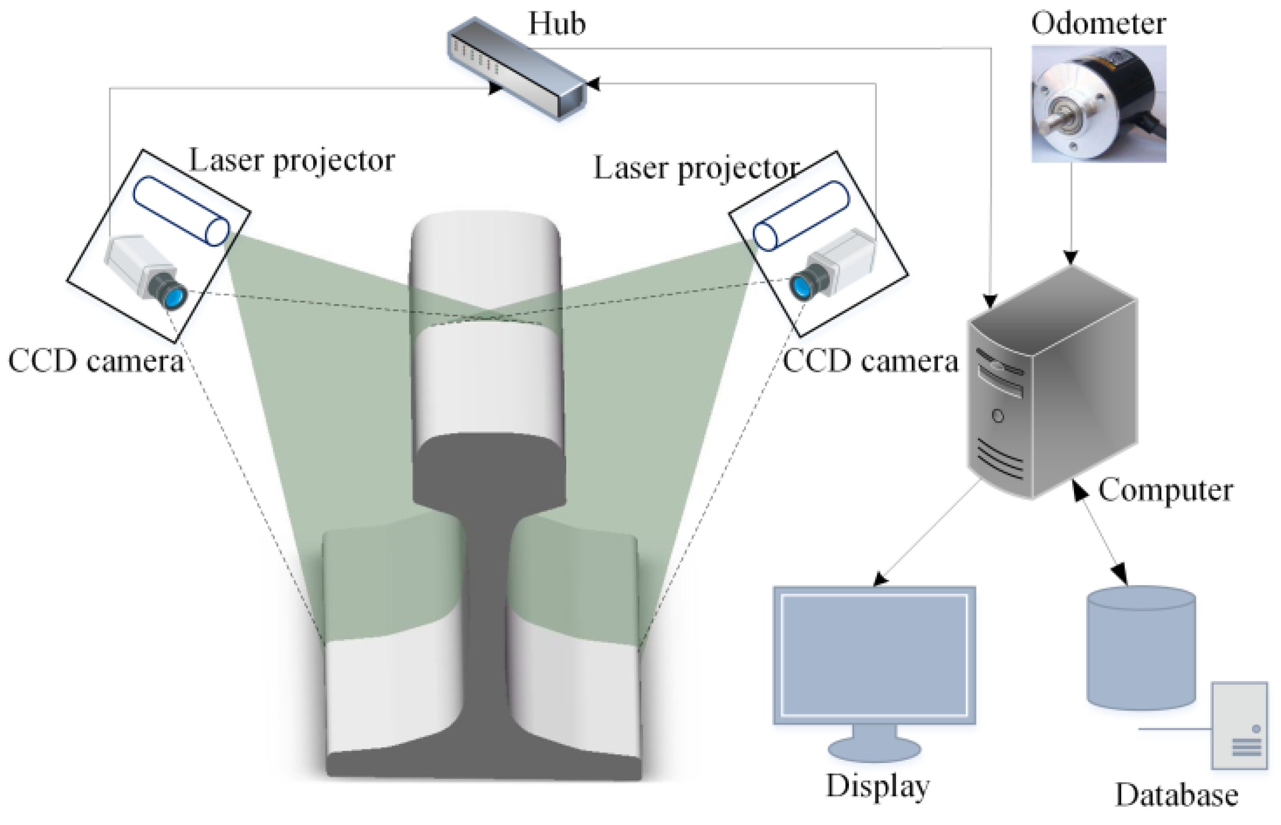
2. Rail Cross-Section Full-Profile Measurement System Based on Binocular Line-Structured Light

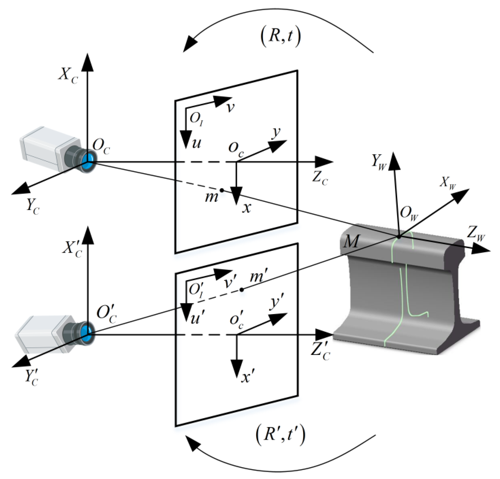
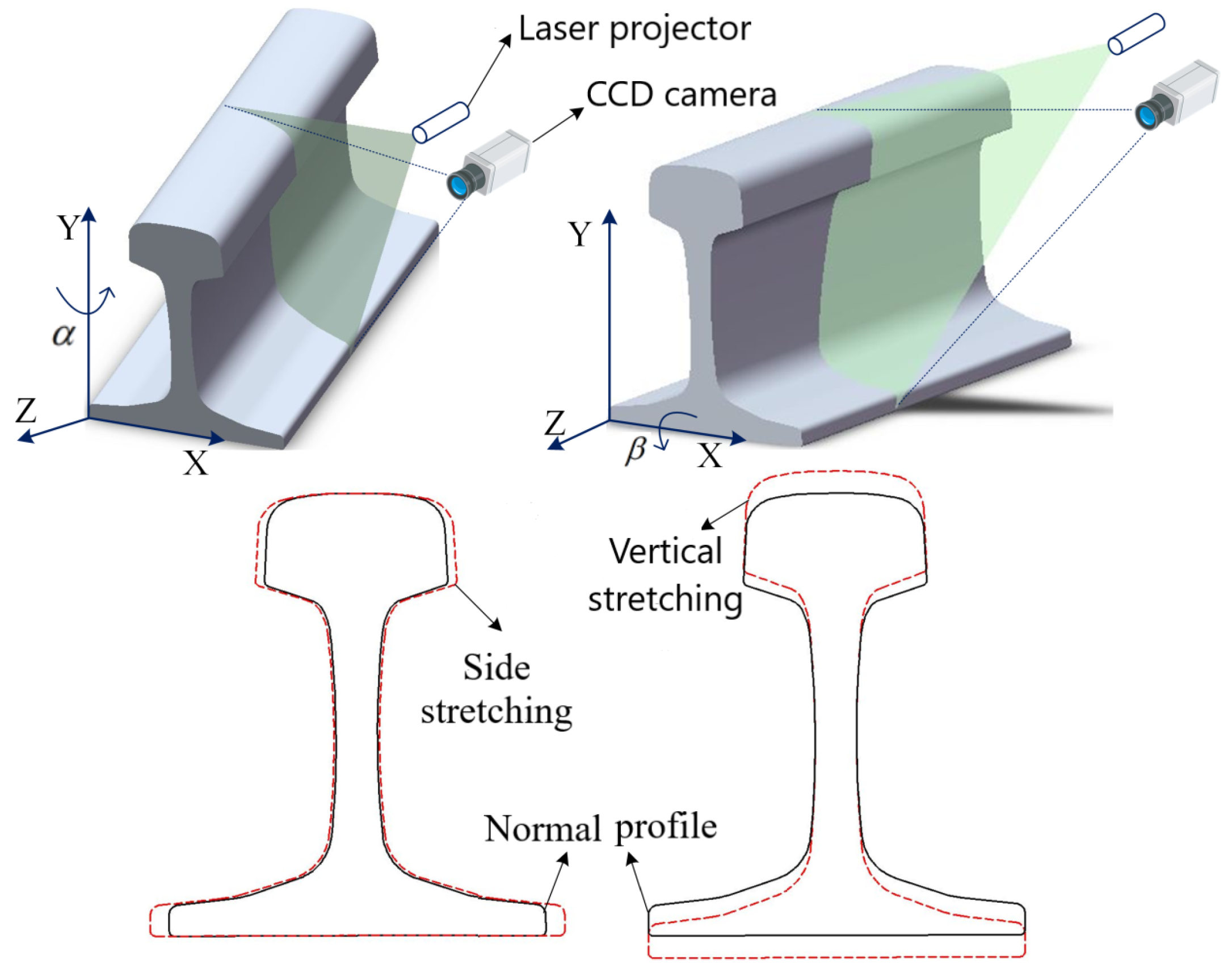
2.1. Binocular Measurement System and Model

The structure of the binocular-structured light-based steel rail cross-section full-profile measurement system is shown in Figure 1. The system consists of a measurement unit comprising two sets of line lasers and CCD cameras, a data switch, an odometer, and a data processing computer. The structured light vision acquisition front-end uses a Basler acA1600-120uc CCD camera with an image resolution of 1600 × 1200. The lens used has a target size of 1/1.8${}^{″}$ and a resolution of 5 million, and the accuracy of the image can be guaranteed. During the inspection, the line lasers are projected vertically onto the surface of the steel rail, forming a curve of full-profile light stripes on the rail section. The odometer triggers the cameras at a fixed frequency to capture the images of the rail profile light stripes. The computer, using an established binocular vision imaging model based on structured light, reconstructs the full profile of the rail section from the captured light stripe images.

The binocular-structured-light vision system model is shown in Figure 2. $O_w{X}_w{Y}_w{Z}_w$ is the world coordinate system, $O_c{X}_c{Y}_c{Z}_c$ and $O_c^{{}^{\prime }}{X}_c^{{}^{\prime }}{Y}_c^{{}^{\prime }}{Z}_c^{{}^{\prime }}$ are the camera coordinate system, $o_{c}xy$ and $o_c^{{}^{\prime }}{x}^{{}^{\prime }}{y}^{{}^{\prime }}$ are the camera imaging plane coordinate system, $o_{1}uv$ and $o_1^{{}^{\prime }}{u}^{{}^{\prime }}{v}^{{}^{\prime }}$ are the camera imaging plane pixel coordinate system, $\left[Rt\right]$ and $\left[R^{\prime }{t}^{\prime }\right]$ are the transformation matrix between the camera coordinate system and the world coordinate system. Suppose point $P_M={(x_w,y_w,z_w)}^T$ is an intersection point M between the light plane and the surface of the steel rail in the world coordinate system, then $P_c={(x_c,y_c,z_c)}^T$ and $p_c^{{}^{\prime }}={(x_c^{{}^{\prime }},y_c^{{}^{\prime }},z_c^{{}^{\prime }})}^T$ are the coordinates of point M in the camera coordinate system, $p_m={(u_m,v_m)}^T$ and $p_m^{{}^{\prime }}={(u_m^{{}^{\prime }},v_m^{{}^{\prime }})}^T$ are the pixel coordinates of the point imaged by the camera. Taking the $O_c{X}_c{Y}_c{Z}_c$ camera as an example, a camera is modeled by the usual pinhole: the relationship between a 3D point M and its image projection m is given by

$$s{\tilde{p}}_m=A{p}_c=A\left[Rt\right]{\tilde{P}}_M$$

(1)

where s is the scale factor, A is the matrix of the camera’s intrinsic parameters, R and t are the rotation matrix and translation vector from the world coordinate system to the camera coordinate system, and ${\tilde{p}}_m$ and ${\tilde{P}}_M$ are the homogeneous coordinates of $p_m$ and $P_M$. In addition, $P_M$ satisfies

$$a{x}_c+b{x}_c+c{z}_c+d=0$$

(2)

where (a, b, c, and d) are the parameters of the light plane in the camera coordinate system.

The light plane in the world coordinate system satisfies

$$Z_W=0$$

(3)

Referring to (1) to (3), the binocular-structured-light vision model can be represented as

$$\left\{\begin{array}{c}s{\tilde{p}}_m=A{P}_c=A\left[Rt\right]{\tilde{P}}_M\hfill \\ a{x}_c+b{x}_c+c{z}_c+d=0\hfill \\ s^{{}^{\prime }}{\tilde{p}}_m^{{}^{\prime }}=A^{{}^{\prime }}{p}_c^{{}^{\prime }}=A^{{}^{\prime }}\left[R^{{}^{\prime }}{t}^{{}^{\prime }}\right]{\tilde{P}}_M\hfill \\ a^{{}^{\prime }}{x}_c^{{}^{\prime }}+b^{{}^{\prime }}{x}_c^{{}^{\prime }}+c^{{}^{\prime }}{z}_c^{{}^{\prime }}+d^{{}^{\prime }}=0\hfill \\ Z_W=0\hfill \end{array}\right.$$

(4)

where the camera’s intrinsic parameters A and $A^{{}^{\prime }}$ can be obtained using the chessboard calibration method [18]. If the external parameters $\left[Rt\right]$ and $\left[R^{{}^{\prime }}{t}^{{}^{\prime }}\right]$ of the transformation from the line-structured-light plane $Z_W=0$ in the world coordinate system to the $O_c{X}_c{Y}_c{Z}_c$ and $O_c^{{}^{\prime }}{X}_c^{{}^{\prime }}{Y}_c^{{}^{\prime }}{Z}_c^{{}^{\prime }}$ camera coordinate systems can be obtained, the unique coordinates of the complete rail profile on the line-structured-light plane $P_M$ in the world coordinate system can be determined.

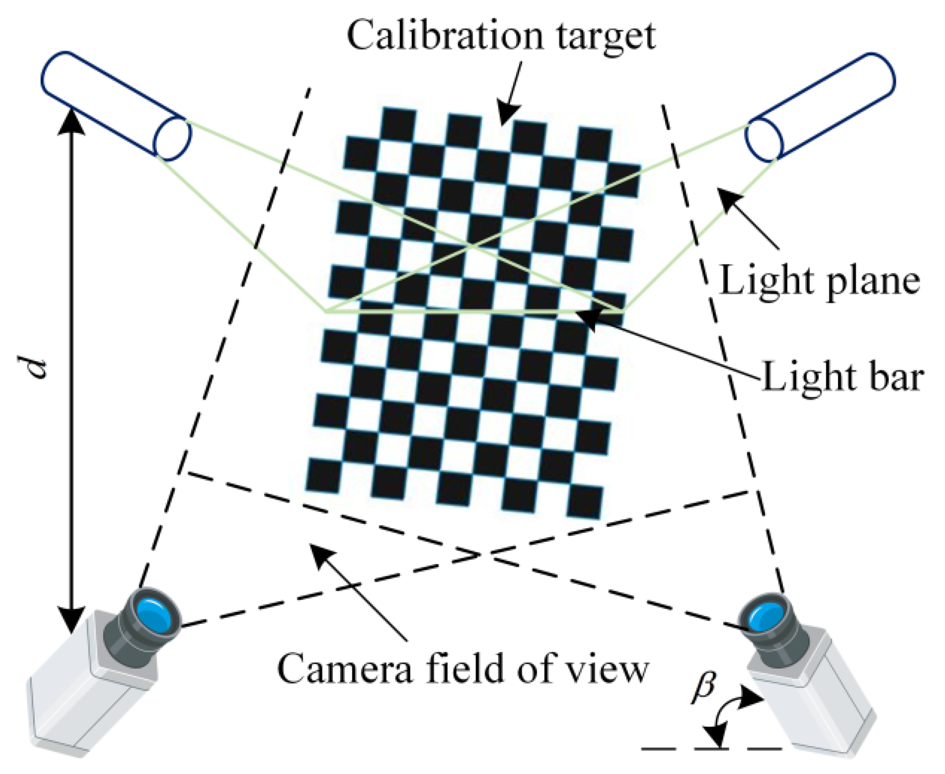
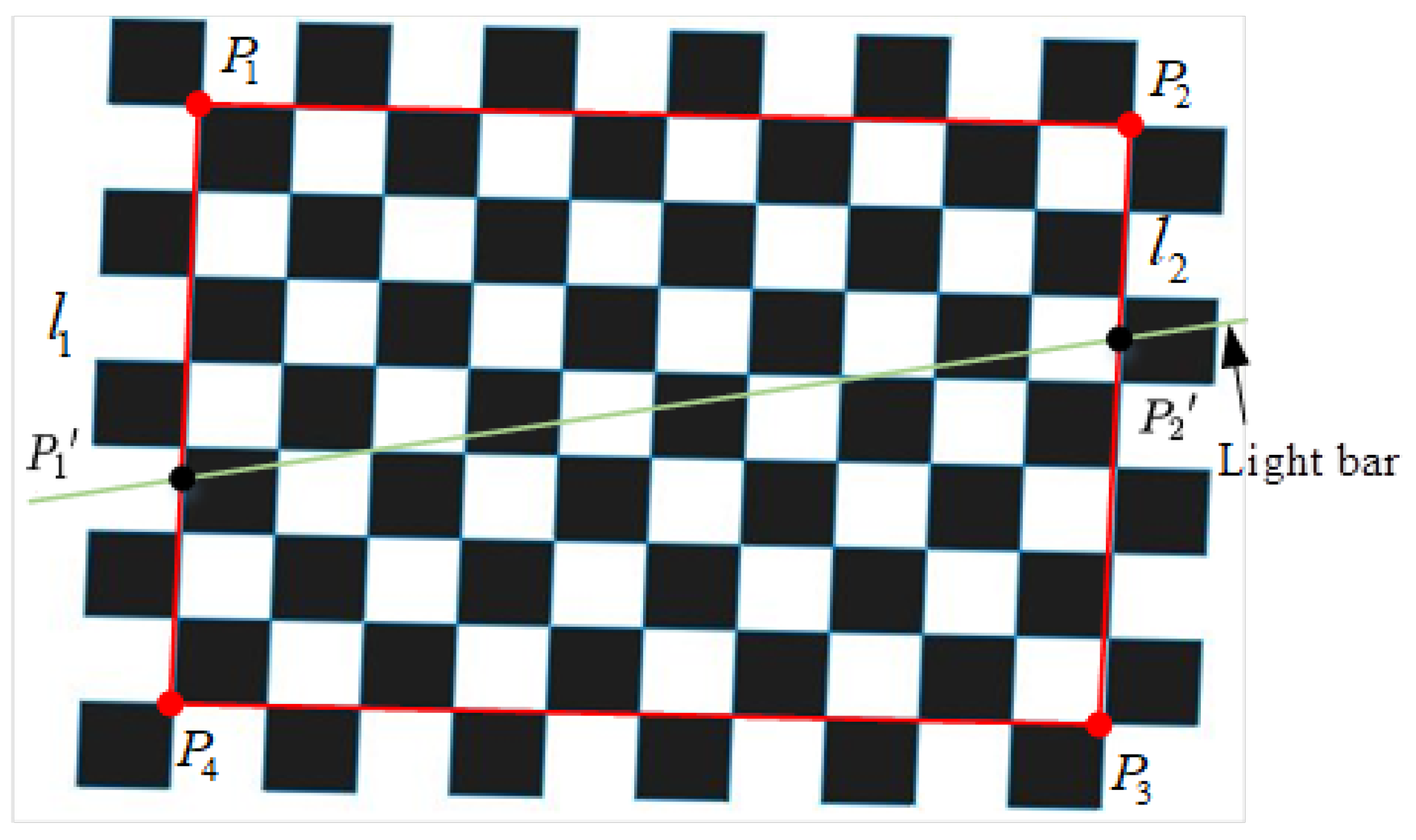
2.2. Determination of the Measurement Plane for Line-Structured Light

To achieve simultaneous calibration of the cameras on both sides of the rail, the checkerboard calibration board is adjusted so that it is within the common field of view of the two cameras. Then, the line projectors on both sides are adjusted to align the light planes, as shown in Figure 3. The cameras and projectors are symmetrically distributed on both sides, and the angle between the camera optical axis and the light plane is approximately $\beta ={60}^{\circ }$. The vertical distance d between the projectors and the cameras is

$$d=fH/h\times sin\beta$$

(5)

where f is the focal length of the camera, H is the height of target, and h is the optical size of camera.

The target plane is fixed in the common viewing area of the cameras on both sides. An image of the target plane is captured, denoted as image $F_i$, and an image of the intersection between the target plane and the line-structured-light plane is captured, denoted as image $F_i^{{}^{\prime }}$. Image $F_i$ is used to extract corner points, while image $F_i^{{}^{\prime }}$ is used to extract feature points formed by the intersection between the line-structured-light plane and the calibration board, the images captured by the cameras on both sides are shown in Figure 4. Then, the target plane is moved i (≥3) times, and the above steps are repeated to obtain i pairs of images.

The chessboard calibration method [18] is used to solve the external parameters $[R_i,t_i]$ and $[R_i^{\prime },t_i^{\prime }]$ that transform each set of captured target planes from the world coordinate system $Z_W=0$ to the coordinate systems of the cameras on both sides; the origin of the world coordinate system is set to the top-left corner point of the target plane. The feature points formed by the intersection of the light stripes and the chessboard target plane are shown in Figure 5 as points $P_1^i$ and $P_2^i$.

In the figure, points $P_1,P_2,P_3$, and $P_4$ represent the four corner points of the target plane, in the image, the corresponding corner points are denoted as $P_{m1},P_{m2},P_{m3}$, and $P_{m4}$. By moving the target plane times, the line-structured-light plane will generate a total of $2m$ feature points in the coordinate systems of the cameras on both sides. The coordinates of feature points $p_1^i,p_2^i$ in the camera coordinate system are as follows:

$$\left\{\begin{array}{c}{P}_{c1}^i=\left[R_i{t}_i\right]P_1^i\hfill \\ P_{c2}^i=\left[R_i{t}_i\right]P_2^i\hfill \\ P_{c1}^{{}^{\prime }i}=\left[R_i^{\prime }{t}_i^{\prime }\right]P_1^i\hfill \\ P_{c2}^{{}^{\prime }i}=\left[R_i^{\prime }{t}_i^{\prime }\right]P_2^i\hfill \end{array}\right.,i=1,2\dots m$$

(6)

In the equation, points $P_1^i$ and $P_2^i$ are unknown and can be obtained through the processing of images $F_i$ and $F_i^{\prime }$. In image $F_i^{\prime }$, the pixel coordinates $(u_j,v_j),j=1,2\dots ,n$ that correspond to the light stripe satisfy the following condition:

$$v=mu+c$$

(7)

The pixel points $(u_j,v_j),j=1,2\dots ,n$ occupied by the light stripe can be extracted from images $F_i$ and $F_i^{\prime }$ using the differential method. Then, the line parameters of the light stripe in the images can be solved using the least squares method:

$$\left\{\begin{array}{c}m=\frac{n(\sum u_j{v}_j)-(\sum u_j)(\sum v_j)}{n(\sum u_j^2)-{(\sum u_j)}^2}\hfill \\ c=\frac{(\sum u_j^2)(\sum v_j)-(\sum u_j)(\sum u_j{v}_j)}{n(\sum u_j^2)-{(\sum u_j)}^2}\hfill \end{array}\right.$$

(8)

The subpixel coordinates of the $P_{m1}{P}_{m2}{P}_{m3}{P}_{m4}$ corner point can be obtained from the $F_i^{\prime }$ image [19]. Using line intersection calculations, the intersection points $P_{m1}^i$ and $P_{m2}^i$ can be determined for the lines formed by the corner points $P_{m1}{P}_{m4}$ and $P_{m2}{P}_{m3}$ in the image, and the lines representing the structure of the light stripe. The chessboard target plane has a square size of 15 mm, according to the projective transformation and the principle of invariant ratios [20], the points $P_{m1}^j$ and $P_{m2}^j$ in the image and their corresponding feature points $P_1^i$ and $P_2^i$ in the world coordinate system satisfy the following relationship:

$$\frac{P_1^i-P_1}{P_1^i-P_4}=\frac{P_{m1}^i-P_{m1}}{P_{m1}^i-P_{m4}},\frac{P_2^i-P_2}{P_2^i-P_3}=\frac{P_{m2}^i-P_{m2}}{P_{m2}^i-P_{m3}}$$

(9)

From (6) to (9), by applying the singular value decomposition (SVD) method to the feature points $P_{c1}^i,P_{c2}^i$ and $P_{c1}^{{}^{\prime }i},P_{c2}^{{}^{\prime }i},i=1,2\dots m$, we can individually fit the equations of the line-structured-light plane in the coordinate systems of the two cameras:

$$\left\{\begin{array}{c}a{x}_c+b{x}_c+c{z}_c+d=0\hfill \\ a^{\prime }{x_c}^{\prime }+b^{\prime }{x_c}^{\prime }+c^{\prime }{z_c}^{\prime }+d^{\prime }=0\hfill \end{array}\right.$$

(10)

Based on Equations (3) and (10), and using the Rodrigues transformation [21], we can calculate the external parameter matrices $\left[Rt\right]$ and $\left[R^{\prime }{t}^{\prime }\right]$, which represent the transformation from the line-structured-light plane to the coordinate systems of the two cameras.

3. Full-Profile Wear Measurement of Rail Section Based on Binocular Line-Structured Light

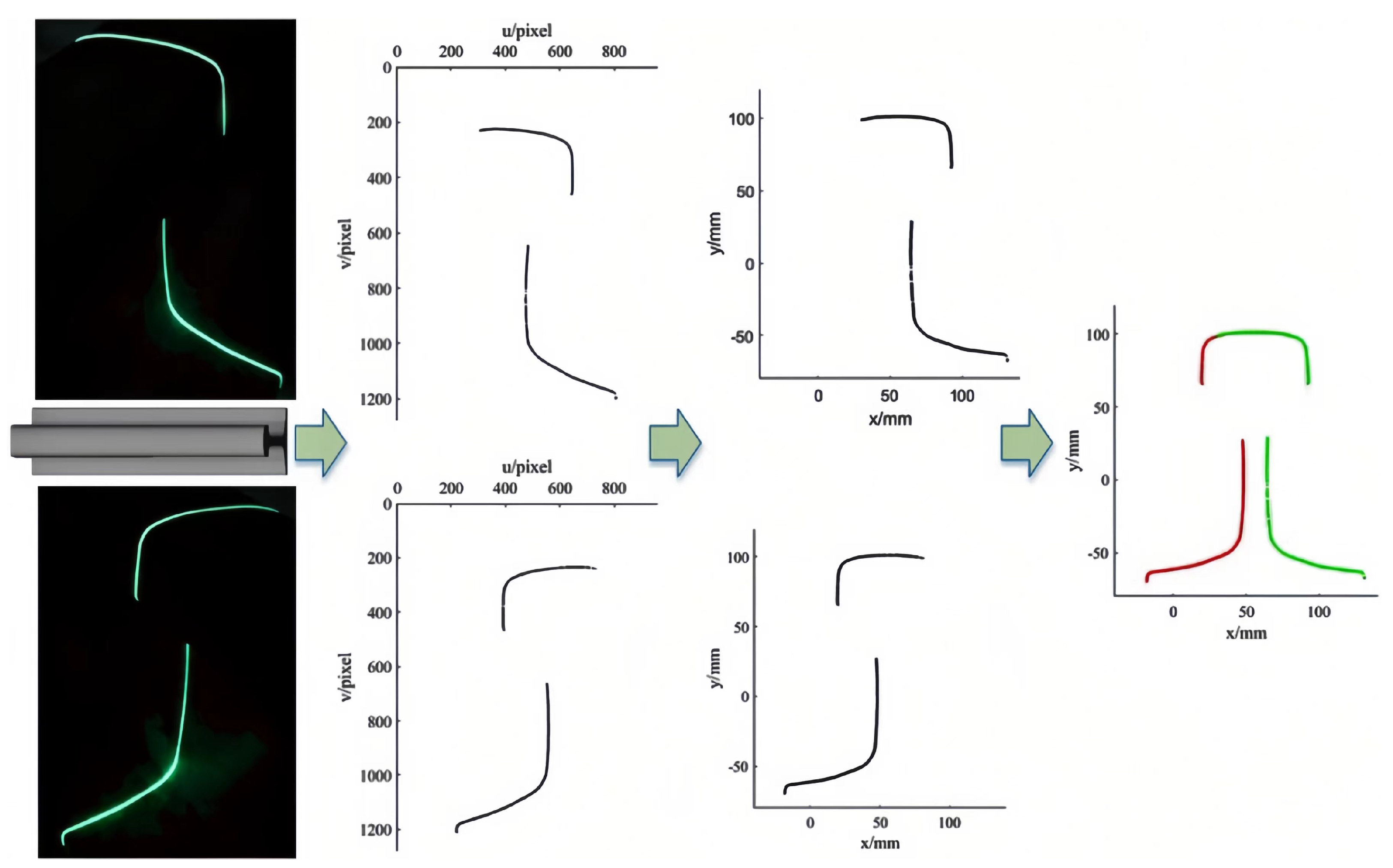
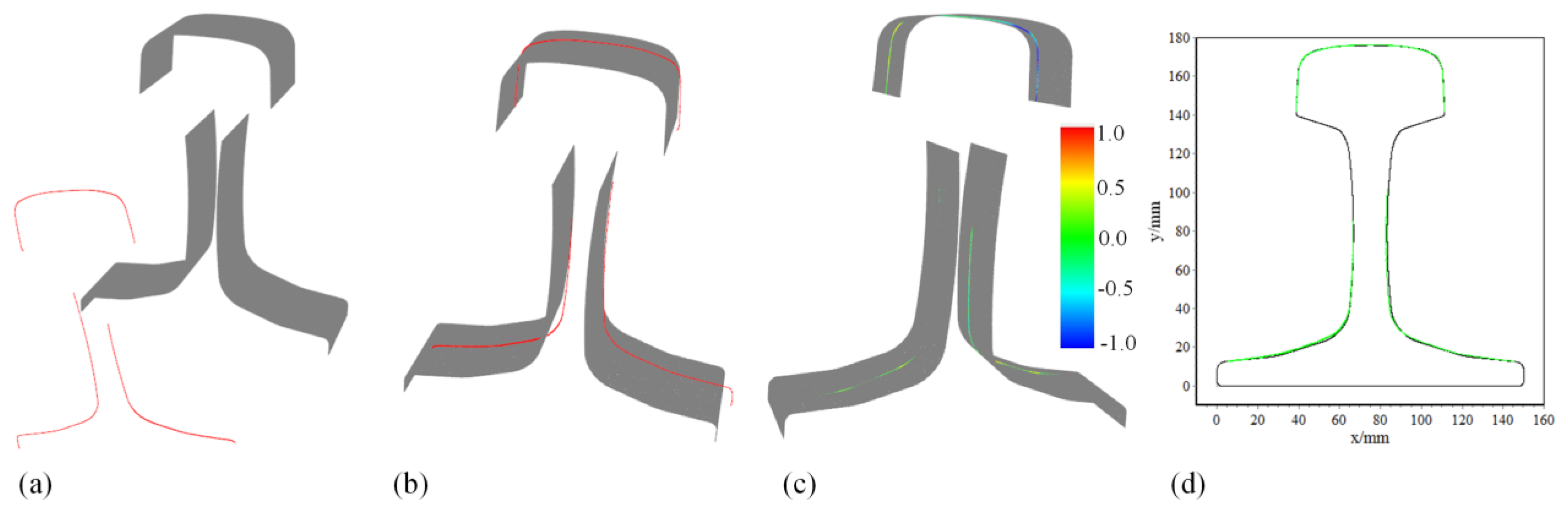
3.1. Extraction of Full Profile of Steel Rail Section

The rail geometry information can be obtained by means of distance measuring equipment such as rail height, rail waist height, rail waist width, and rail waist inclination, and the curve shape information can be obtained using a laser scanner. First, the contour images of the inner and outer sides of the steel rail are captured. Then, the subpixel coordinates of the center points of the steel rail contour light stripes are extracted [22,23]. Based on the established dual-camera vision model and the calibration of the line-structured-light plane’s external parameters, the steel rail contour points on the line-structured-light plane are calculated using Equation (11):

$$\left\{\begin{array}{c}{\tilde{P}}_M=s{\left[Rt\right]}^{-1}{A}^{-1}{\tilde{P}}_m\hfill \\ {\tilde{P}}_M^{{}^{\prime }}=s{\left[R^{{}^{\prime }}{t}^{{}^{\prime }}\right]}^{-1}{A}^{-1}{\tilde{P}}_m^{{}^{\prime }}\hfill \end{array}\right.$$

(11)

To convert the subpixel coordinates of the center points of the rail profile light stripes in the image to the coordinates of the actual rail profile points on the measured light plane in the world coordinate system, the curved shape information of the rail is obtained using a laser scanner. The two locations on the top and bottom of the rail can be marked as “right” and “left”, respectively. Then, the image undergoes median filtering and subpixel processing to obtain the contours of one side of the rail. Based on this, the complete contour of the rail on both sides is merged, as shown in Figure 6.

3.2. Measurement of Railhead Contour Based on Two-Step Method

According to the “Maintenance Rules for Ballastless Track of High-speed Railway” [24], the measurement of vertical wear on the rail is taken at a width of one-third of the rail’s top surface, and the measurement of side wear on the rail is taken 16 mm below the rail’s running surface. As shown in Figure 7, $W_V$ represents the vertical wear of the rail, and $W_H$ represents the side wear of the rail. In general, by comparing the measured rail profile with the standard 2D profile, we can obtain $W_V$ and $W_H$. However, the visual measurement system is installed on a moving train, and the vibrations of the train body can cause the random deflection of the line-structured-light measurement plane.

As shown in Figure 8, a yaw angle deviation around the Y-axis, denoted as $\alpha$, results in the measured rail profile being horizontally stretched compared to the standard rail profile. Similarly, a pitch angle deviation around the X-axis, denoted as $\beta$, leads to the measured rail profile being vertically stretched compared to the standard profile. Directly comparing the measured rail profile obtained under the train’s vibration with the standard 2D rail profile will introduce measurement deviation. Therefore, the two-step method for measuring the railhead profile is adopted, which involves comparing the measured full rail profile with a standard 3D steel rail point cloud model in three-dimensional space. This approach helps to eliminate the influence of vibrations during the measurement process. Please refer to Section 3.2.1 and Section 3.2.2 for detailed procedures.

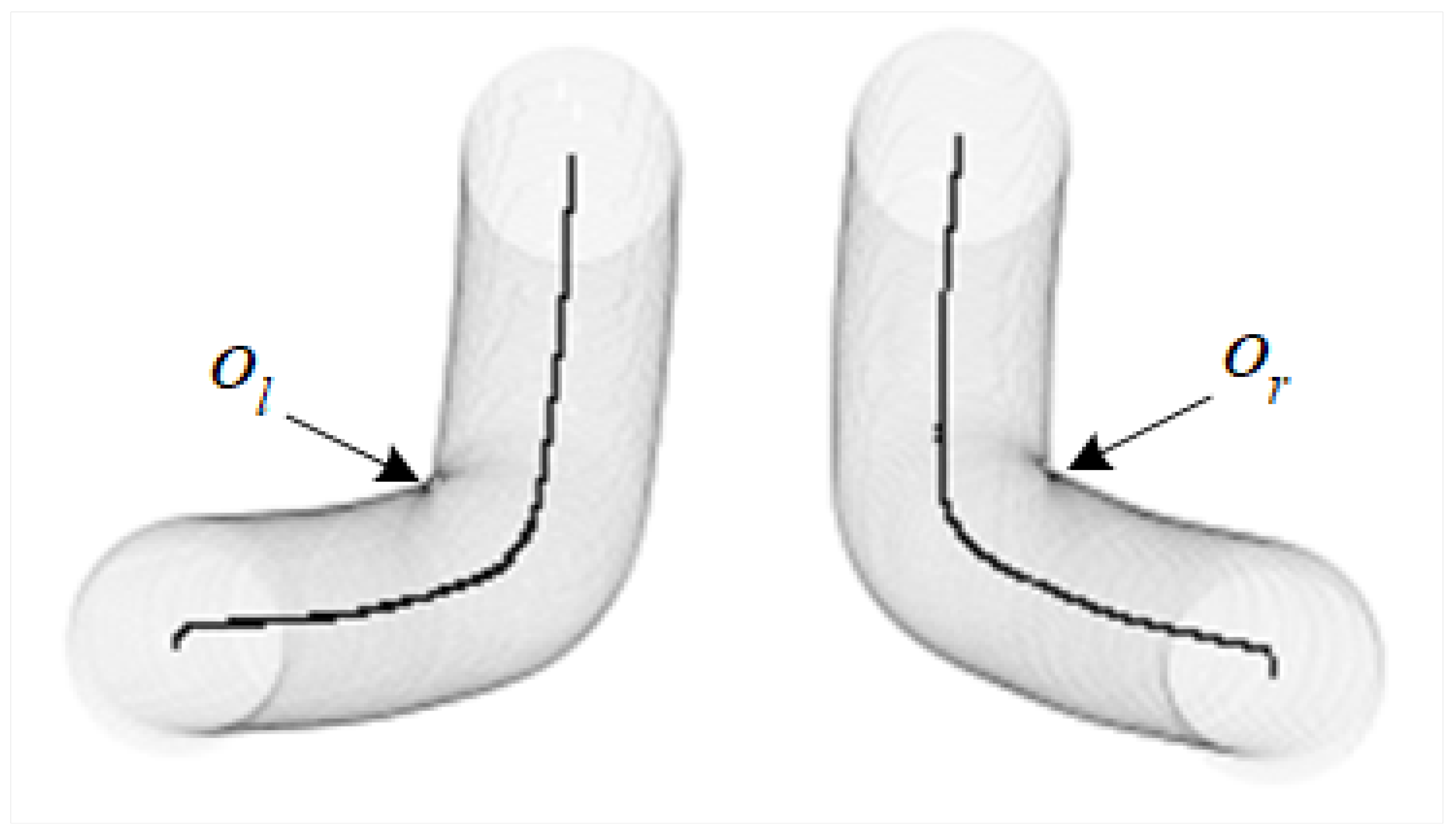
3.2.1. Step 1: Initial Alignment of Rail Waist Contour Based on Rail Waist Feature Vectors

Due to the random deviation of the line-structured-light plane, the initial position of the measured steel rail profile in three-dimensional space differs significantly from the standard rail model. This misalignment prevents accurate alignment, requiring adjustment of the initial position of the measured rail profile to achieve initial registration with the standard rail model. By analysis, the complete rail profile can be divided into the railhead and rail waist sections, with the rail waist section experiencing no wear during actual operation. Therefore, the rail waist profile can be used as the reference. Two different feature vectors are formed by connecting the centers of the small circular arcs on both sides of the rail waist profile of the measured rail profile and the standard rail model, respectively, and the initial registration of the measured rail profile and the standard rail model is realized by aligning the two feature vectors. The specific process is as follows:

First, to minimize interference during the alignment between the measured rail profile and the standard rail model, the railhead bottom surface and rail bottom surface data of the standard steel rail model are removed before matching with the measured rail profile. Then, the standard rail model is transformed into a point cloud model. Specifically, for each triangle in the standard steel rail model with three vertices A, B, and C, a random uniformly distributed point cloud $Q_k,k=1,2\dots$ is generated on the surface of the triangle.

$$Q_k=A+s\overrightarrow{AB}+t\overrightarrow{AC}$$

(12)

where s and t are random numbers in [0, 1], if $s+t>1$, then $s=1-s$ and $t=1-t$ [25]. Establish a Kd-tree index for the measured rail profile points to enable fast searching based on neighborhood relationships. Specifically, the measured rail profile points are denoted as Q, with the railhead contour points represented by $Q_H$, and the rail waist contour points represented by $Q_W$. Due to the significant distance between $Q_H$ and $Q_W$, we can use Euclidean clustering to segment and extract them.

Then, as shown in Figure 9, the approximate centroid coordinates of the small arc contours on both sides of the steel rail waist can be extracted using techniques such as Hough circle detection. The radius of the small arc contour is r = 20 mm. The centroid coordinates $o_r$ and $o_l$ can be obtained, and the position of the centroid can be determined based on the grayscale values in the image. Specifically, in the steel rail waist curve, where each pixel point represents 1 mm, we can draw a circle with radius $r=20\pi$ centered at the steel rail waist contour point, and the value of the corresponding pixel point increases by 1 when the arc passes through the pixel point. The approximate coordinates of the maximum pixel value point correspond to the centroid coordinates $o_r$ and $o_l$ of the small arc contour;the resulting steel rail waist feature point vector is denoted as $\overrightarrow{o_l{o}_r}$. Furthermore, for the standard rail model, the corresponding approximate coordinates on both sides of the rail waist contour are denoted as $O_R$ and $O_L$, and the corresponding rail waist feature point vector is $\overrightarrow{O_R{O}_L}$. The corresponding points of the measured steel rail contour after initial registration are denoted as $Q^{\prime }$, the rail waist contour points become $Q_W^{\prime }$, the rotation matrix and translation vector for the initial registration are represented as $R_1$ and $t_1$, the detailed solution process can be found in Equations (13)–(15).

$$\left\{\begin{array}{c}{Q}^{\prime }=R_{1}Q+t_1\hfill \\ {Q_W}^{\prime }=R_1{Q}_W+t_1\hfill \end{array}\right.$$

(13)

$$\left\{\begin{array}{c}{R}_1=I+sin\left(\theta \right)K+(1-cos\left(\theta \right))K^2\hfill \\ t_1=O_L-o_l\hfill \end{array}\right.$$

(14)

$$\left\{\begin{array}{c}k=\overrightarrow{o_l{o}_r}\times \overrightarrow{O_R{O}_L}\hfill \\ \theta =acos\frac{\overrightarrow{o_l{o}_r}·\overrightarrow{O_R{O}_L}}{∥\overrightarrow{o_l{o}_r}∥\ast ∥\overrightarrow{O_R{O}_L}∥}\hfill \end{array}\right.$$

(15)

In this formula, k represents the rotation axis vector for the rotation transformation, $\theta$ represents the rotation angle, K represents the cross-product matrix of k, and I represents the identity matrix.

3.2.2. Step 2: Accurate Measurement of Railhead Profile Based on ICP Algorithm and Model Registration

Using the initially aligned measured contour as a reference, and using the the ICP (iterative closest point) algorithm to achieve precise registration of the measured contour and the standard rail model, this ultimately enables the measurement of the railhead profile. In the ICP algorithm for precise registration, the total number of iterations [26], total deviation, and threshold for the difference between consecutive deviations are set to limit the number of iterations. The algorithm utilizes singular value decomposition (SVD) to estimate the rigid transformation. The rotation matrix and translation vector for precise registration are denoted as $R_2$ and $t_2$, respectively, to achieve the following transformation:

$$f(R_2,t_2)=\sum {∥Q_k-(R_2{Q}^{\prime }+t_2)∥}^2=min$$

(16)

Finally, the transformation of the measured full rail contour points Q is given by:

$$Q^{″}=R_2(R_{1}Q+t_1)+t_2$$

(17)

Projecting the full rail contour points $Q^{″}$ onto a plane perpendicular to the longitudinal direction of the rail and establishing a Kd-tree index, we can use the nearest neighbor point search to find the distances between the measured rail contour and the standard rail contour. This allows us to calculate the rail’s overall wear condition based on the contour.

In summary, the alignment and comparison process between the measured rail contour points and the standard rail point cloud is shown in Figure 10. The process involves two steps: initial alignment and precise alignment. (a) The measured steel rail’s full contour points are imported into the initial state of the standard steel rail point cloud in 3D space; (b) based on the feature vector formed by connecting the centers of the small circular arcs on both sides of the steel rail contour, the initial alignment between the measured steel rail contour and the standard steel rail model is performed; (c) the precise alignment is achieved by aligning the measured steel rail’s full contour points with the standard steel rail point cloud model. The measured steel rail’s waist section fits perfectly with the standard steel rail point cloud model, enabling accurate measurement and detection of railhead contour wear.

4. Experiment and Analysis

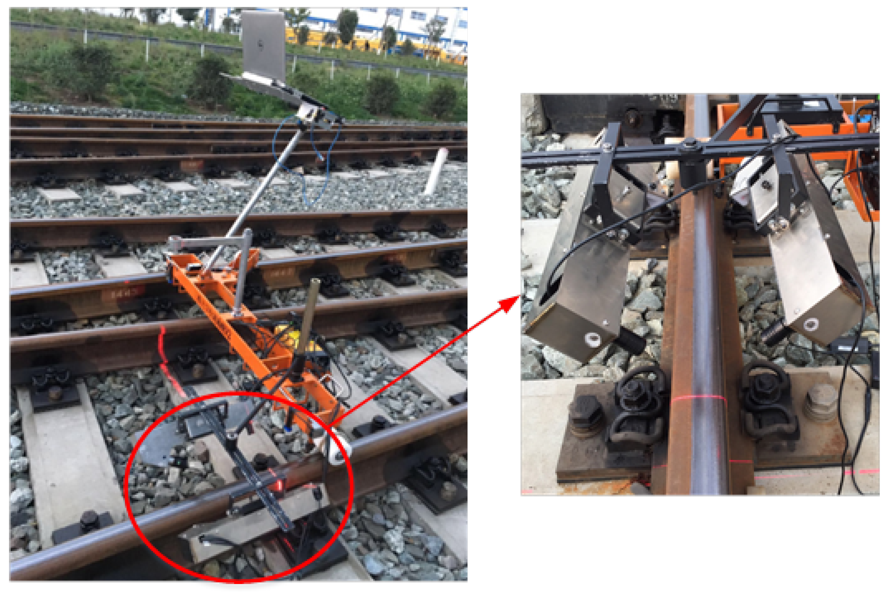
4.1. Test Experiment Platform

The measurement system was tested at the railway maintenance base of the railway bureau, as shown in Figure 11. The vision sensor was installed on the upper side of the railhead, about 70 mm above, and the vision sensor and line laser were fixed at a certain relative angle. The resolution of the vision sensor was $1600\times 1200$, and the system was capable of capturing and processing rail contour images, system calibration, and measuring rail wear on the entire contour. The experimental process included the following steps: first, verifying the accuracy of the system’s stereo calibration method [27]; then, using the proposed binocular vision measurement system and wear gauge measurement, comparing the vertical and side wear of the same rail to validate the measurement accuracy.

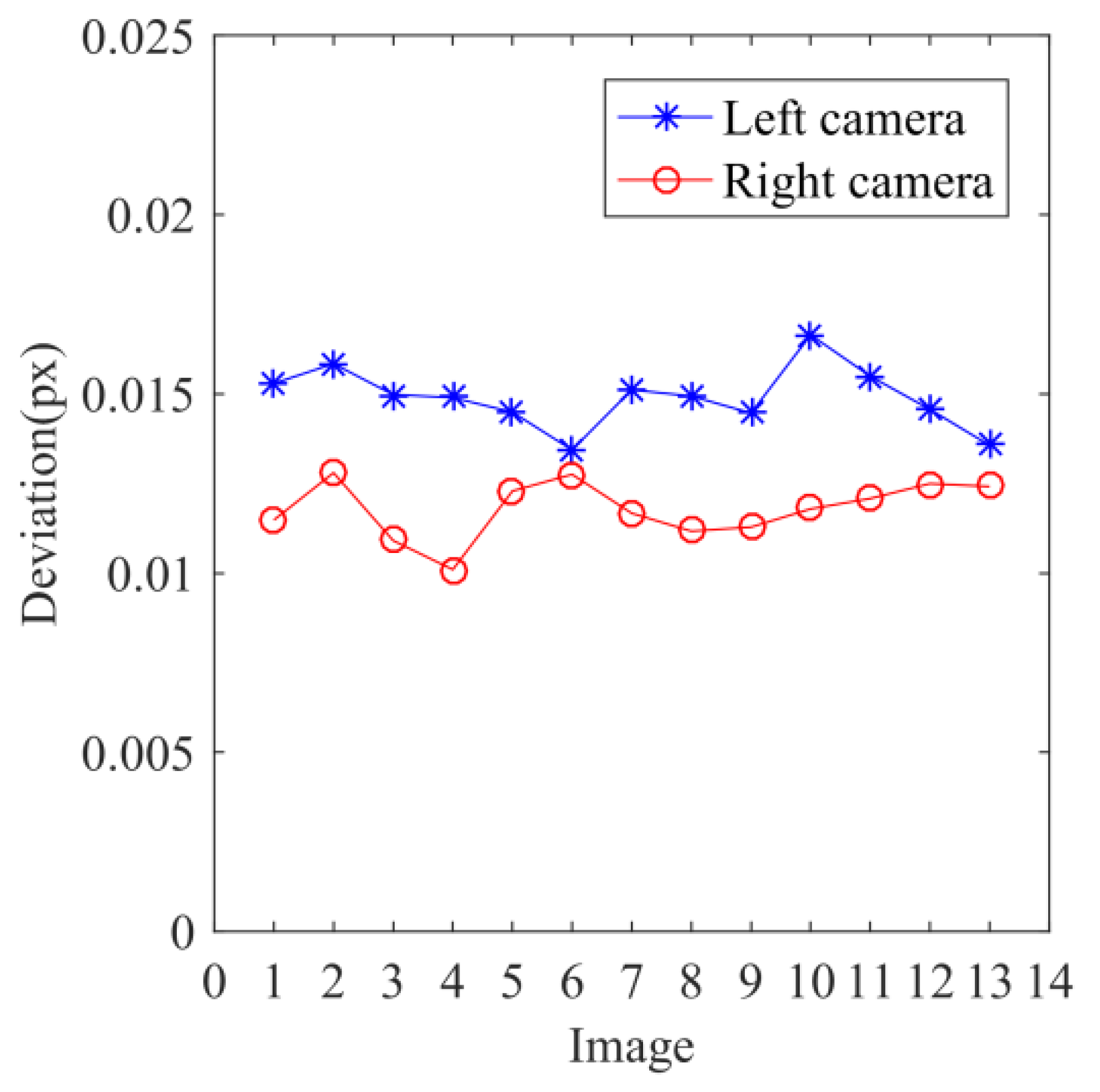
4.2. Calibration of Measurement System and Accuracy Analysis

The line-structured-light binocular camera system employs a $9\times 12$ chessboard calibration board with square size of $15\times 15$ mm. Thirteen sets of images of light stripe targets are captured using the two cameras. The method described in Section 2.2 is used to extract feature points at the intersections of the light stripes and the chessboard grid. The fitted equations of the light planes in the coordinate systems of the left and right cameras are as follows:

$$\left\{\begin{array}{c}-0.476x_c-0.543x_c+0.692z_c-196.001=0\hfill \\ 0.391{x_c}^{\prime }-0.528{x_c}^{\prime }+0.754{z_c}^{\prime }-202.922=0\hfill \end{array}\right.$$

(18)

The calculated internal parameters A and $A^{\prime }$ of the two cameras, as well as the external parameters $[R,t]$ and $[R^{\prime },t^{\prime }]$ of the line-structured-light plane, are shown in

Table 1. Results of camera calibration parameters of left and right cameras.

Name	Solution Results
Internal External	$A=\left[\begin{array}{ccc}1899.792& 0& 785.809\\ 0& 1898.065& 621.232\\ 0& 0& 1\end{array}\right]$
	$A^{\prime }=\left[\begin{array}{ccc}1904.880& 0& 804.499\\ 0& 1904.684& 613.186\\ 0& 0& 1\end{array}\right]$
External Parameters	$[R,t]=\left[\begin{array}{cccc}0.877& -0.236& 0.418& -52.677\\ -0.064& 0.806& 0.588& 8.064\\ -0.476& -0.543& 0.692& 253.306\end{array}\right]$
	$[R^{\prime },t^{\prime }]=\left[\begin{array}{cccc}0.920& 0.240& -0.309& -95.225\\ -0.018& 0.815& 0.579& -24.717\\ 0.391& -0.528& 0.754& 301.256\end{array}\right]$

.

In order to evaluate the calibration accuracy of the line-structured-light stereo camera system, and to verify the feasibility of the system, this paper proposes an analysis of the calibration errors of the cameras’ internal parameters and the fitting degree of the line-structured-light plane. By using the calibration of the planar target, the cameras’ internal and external parameters are obtained. The corner coordinates of the planar target in the world coordinate system are projected onto the images and compared with the corresponding corner coordinates in the images. The deviations of each image captured by the left and right cameras are shown in Figure 12. The overall average deviations are 0.0149 px and 0.0118 px, respectively.

In the coordinate systems of the left and right cameras, the distance deviations between the line-structured-light plane fitted using SVD decomposition and the feature points are shown in Figure 13, and only the edge points within the plane have relatively larger errors due to the quality of the projected line-structured light. The evaluation parameters for the fitting of the line-structured-light plane are shown in

Table 2. Fitting plane evaluation parameters.

	Coordinate System of the Left Camera	Coordinate System of the Right Camera
Sum of squared errors (SSE)	2.358	1.761
Coefficient of determination	0.9999	0.9999
(R-square)
Standard deviation (RMSE)	0.3202	0.2767

, where a determination coefficient close to 1 indicates a good fitting degree of the line-structured-light plane.

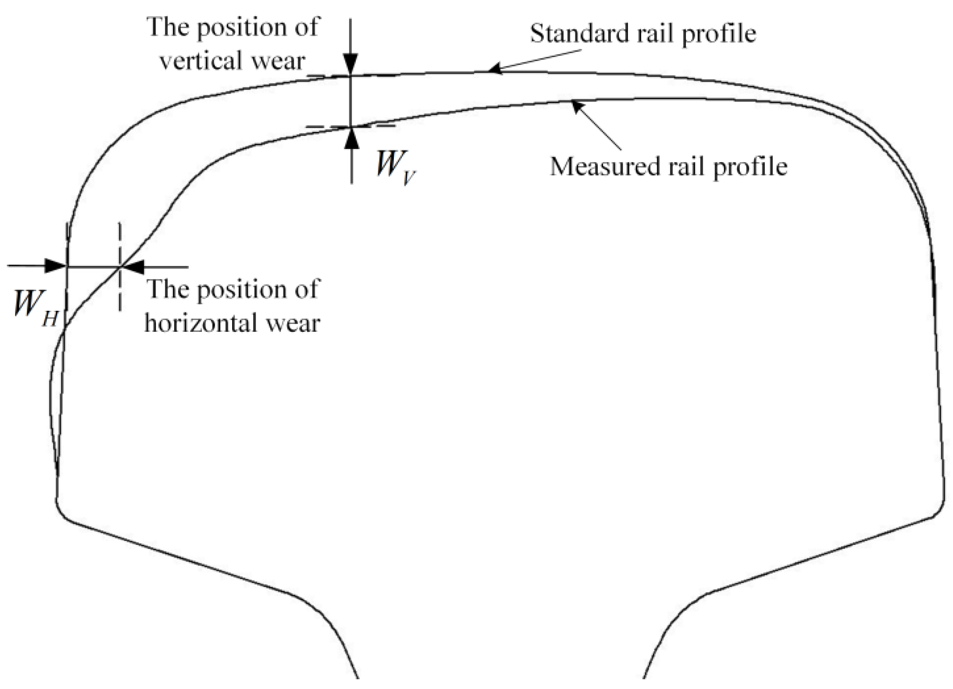
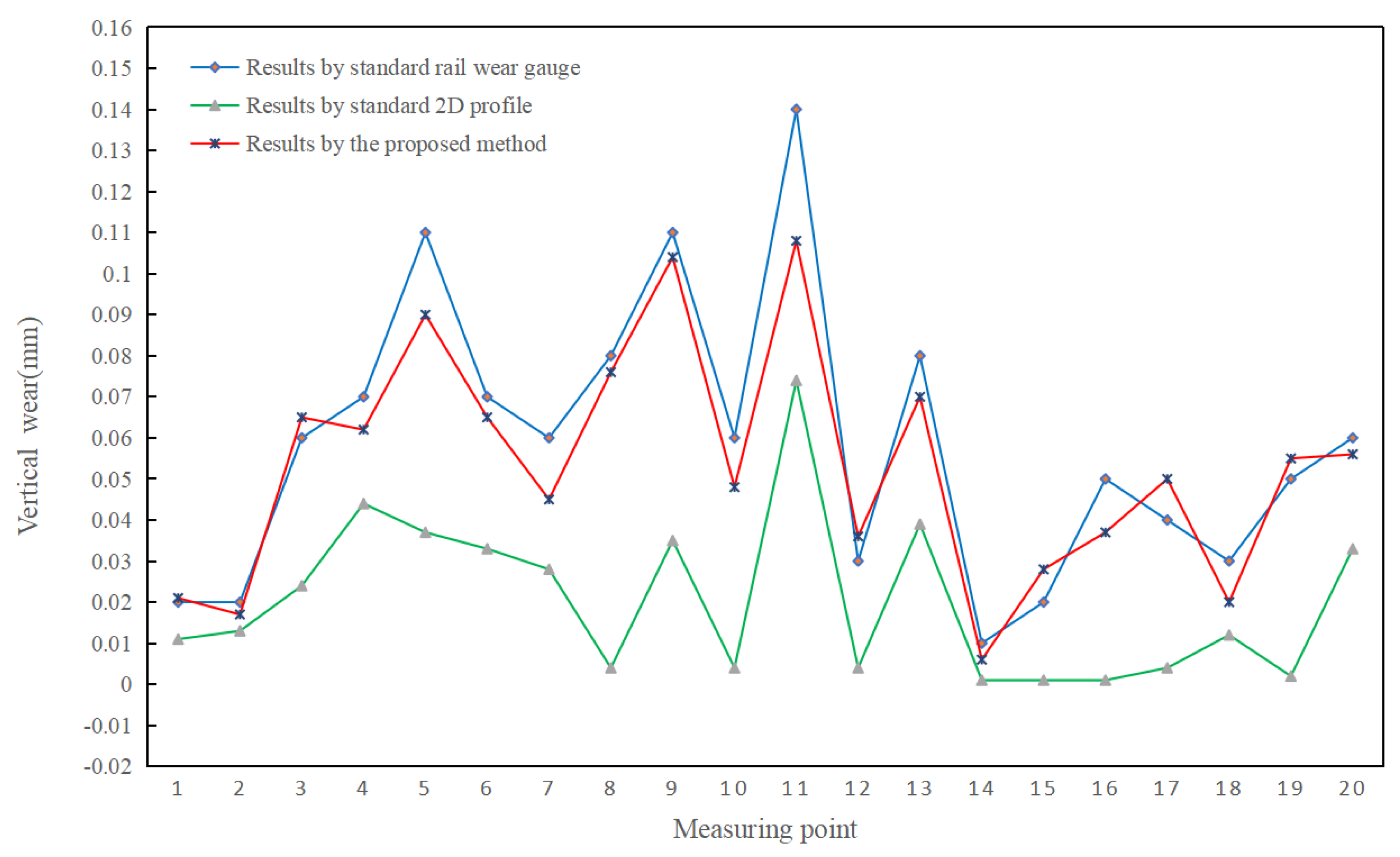
4.3. Analysis of Rail Wear Measurement Accuracy

For the measurement of one section of the 60# steel rail at 20 different positions, the rail wear gauge, the standard rail-based 2D contour measurement and the proposed method in this paper were used. Among them, the cameras used in this experiment have a resolution of 1600 × 1200. The field of view of each camera is approximately 167 × 122 units, and the pixel accuracy is 0.1 mm/pixel. The measurement accuracy for rail wear using the gauge is 0.01 mm, which is one order of magnitude higher than the image accuracy. The vertical wear and side wear obtained based on the rail wear gauge measurement are shown in

Table 3. Results of wear measurement for 60 kg/m rail.

	Results by Standard Rail Wear Gauge		Results by Standard 2D Profile				Results by the Proposed Method
No	Vertical Wear	Side Wear	Vertical Wear	Deviation	Side Wear	Deviation	Vertical Wear	Deviation	Side Wear	Deviation
1	0.020	−0.390	0.011	−0.009	−0.601	−0.211	0.021	0.001	−0.455	−0.065
2	0.020	−0.410	0.013	−0.007	−0.511	−0.101	0.017	−0.003	−0.402	0.008
3	0.060	−0.350	0.024	−0.036	−0.461	−0.111	0.065	0.005	−0.353	−0.003
4	0.070	−0.320	0.044	−0.026	−0.428	−0.108	0.062	−0.008	−0.305	0.015
5	0.110	−0.340	0.037	−0.073	−0.408	−0.068	0.090	−0.020	−0.350	−0.010
6	0.070	−0.300	0.033	−0.037	−0.428	−0.128	0.065	−0.005	−0.301	−0.001
7	0.060	−0.310	0.028	−0.032	−0.399	−0.089	0.045	−0.015	−0.286	0.024
8	0.080	−0.230	0.004	−0.076	−0.261	−0.031	0.076	−0.004	−0.173	0.057
9	0.110	−0.350	0.035	−0.075	−0.441	−0.091	0.104	−0.006	−0.340	0.010
10	0.060	−0.390	0.004	−0.056	−0.490	−0.100	0.048	−0.012	−0.305	0.085
11	0.140	−0.220	0.074	−0.066	−0.292	−0.072	0.108	−0.032	−0.244	−0.024
12	0.030	−0.260	0.004	−0.026	−0.365	−0.105	0.036	0.006	−0.264	−0.004
13	0.080	−0.240	0.039	−0.041	−0.296	−0.056	0.070	−0.010	−0.190	0.050
14	0.010	−0.430	0.001	−0.009	−0.474	−0.044	0.006	−0.004	−0.383	0.047
15	0.020	−0.440	0.001	−0.019	−0.469	−0.029	0.028	0.008	−0.374	0.066
16	0.050	−0.380	0.001	−0.049	−0.375	0.005	0.037	−0.013	−0.292	0.088
17	0.040	−0.210	0.004	−0.036	−0.248	−0.038	0.050	0.010	−0.177	0.033
18	0.030	−0.050	0.012	−0.018	−0.128	−0.078	0.020	−0.010	−0.002	0.048
19	0.050	−0.180	0.002	−0.048	−0.316	−0.136	0.055	0.005	−0.267	−0.087
20	0.060	−0.310	0.033	−0.027	−0.428	−0.118	0.056	−0.004	−0.361	−0.051
MAD (mm)				0.038		0.086		0.009		0.039
RMSE (mm)				0.046		0.097		0.011		0.048

.

There was no obvious data fluctuation in the two groups of data. Therefore, the rail wear gauge measurement data are taken as the reference standard, and the measurement results obtained from the standard rail-based 2D contour measurement and the proposed method in this paper are compared with it. The measurement results are shown in Table 3.

Table 3 shows that compared to the measurement results of the rail wear gauge, the average absolute errors of vertical wear for the two methods are 0.038 mm and 0.009 mm, and the average absolute errors of the side wear measurements are 0.086 mm and 0.039 mm, respectively. The root mean square errors of the vertical wear measurements are 0.046 mm and 0.011 mm, and the root mean square errors of the side wear measurements are 0.097 mm and 0.048 mm, respectively. The proposed method in this paper exhibits smaller average absolute deviations and root mean square errors for both vertical and side wear measurements compared to the results obtained from the standard rail-based 2D contour measurement.

Furthermore, the measurements using the proposed method are closer to the standard measurements obtained from the rail wear gauge, as shown in Figure 14 and Figure 15.

The method proposed in this paper for measuring the railhead contour, has the ability to correct measurement errors caused by random deviations in the measurement plane of the line-structured light. By bringing the measured steel rail’s complete contour into a 3D space and comparing it with the standard 3D point cloud model of the steel rail, the wear can be accurately measured. This approach eliminates the influence of vibrations during the measurement process, and obtains more precise wear measurements.

5. Conclusions

In this paper, a full profile of rail cross-section measurement method based on line-structured light was established, and further, a coarse alignment and precise registration approach was proposed for measuring the railhead contour. The method involved comparing the measured rail contour with a three-dimensional point cloud model of a standard steel rail to obtain rail wear measurements and mitigate the influence of light plane deviations caused by vibrations during the measurement process. The experiments demonstrated the following conclusions: (1) The establishment of the binocular line-structured-light vision system model, with a camera’s internal parameter calibration deviation of approximately 0.01px and a fitting degree of the line-structured-light plane reaching 0.9999, validated the feasibility of the binocular calibration method. (2) The proposed full profile of rail cross-section measurement method based on line-structured light and stereo vision achieved accurate measurement of the railhead contour in a two-step process. The on-site comparative measurement tests showed that the average absolute error in the vertical wear measurement obtained through this method was 0.009 mm, and the average absolute error in the side wear measurement was 0.039 mm. This measurement method effectively corrected measurement plane deviations and met the accuracy requirements for rail wear measurement.

References

1. Wang, C.; Zeng, J. Combination-Chord Measurement of Rail Corrugation Using Triple-Line Structured-Light Vision: Rectification and Optimization. IEEE Trans. Intell. Transp. Syst. 2021, 22, 7256–7265. [Google Scholar] [CrossRef]
2. Minbashi, N.; Bagheri, M.; Golroo, A.; Arasteh Khouy, I.; Ahmadi, A. Turnout degradation modelling using new inspection technologies: A literature review. In Current Trends in Reliability, Availability, Maintainability and Safety: An Industry Perspective; Springer: Cham, Switzerland, 2016; pp. 49–63. [Google Scholar]
3. Steinbuch, M.; Henselmans, R. Non-contact Measurement Machine for Freeform Optics. Macromolecules 2009, 35, 607–624. [Google Scholar]
4. Modjarrad, A. Non-contact measurement using a laser scanning probe. In-Process Optical Measurements. SPIE 1989, 1012, 229–239. [Google Scholar]
5. Giri, P.; Kharkovsky, S. Detection of Surface Crack in Concrete Using Measurement Technique with Laser Displacement Sensor. IEEE Trans. Instrum. Meas. 2016, 65, 1951–1953. [Google Scholar] [CrossRef]
6. Alippi, C.; Casagrande, E.; Scotti, F.; Piuri, V. Composite real-time image processing for railways track profile measurement. IEEE Trans. Instrum. Meas. 2000, 49, 559–564. [Google Scholar] [CrossRef] [Green Version]
7. Ran, Y.; He, Q.; Feng, Q.; Cui, J. High-Accuracy On-Site Measurement of Wheel Tread Geometric Parameters by Line-Structured Light Vision Sensor. IEEE Access 2021, 9, 52590–52600. [Google Scholar] [CrossRef]
8. Chugui, Y.; Verkhoglyad, A.; Poleshchuk, A.; Korolkov, V.; Sysoev, E.; Zavyalov, P. 3D Optical Measuring Systems and Laser Technologies for Scientific and Industrial Applications. Meas. Sci. Rev. 2013, 13, 322–328. [Google Scholar] [CrossRef] [Green Version]
9. Guerrieri, M.; Parla, G.; Celauro, C. Digital image analysis technique for measuring steel rail defects and ballast gradation. Meas. J. Int. Meas. Confed. 2018, 113, 137–147. [Google Scholar] [CrossRef]
10. Liu, Z.; Sun, J.; Wang, H.; Zhang, G. Simple and fast rail wear measurement method based on structured light. Opt. Lasers Eng. 2011, 49, 1343–1351. [Google Scholar] [CrossRef]
11. Wang, C.; Liu, H.; Ma, Z.; Zeng, J. Dynamic inspection of rail wear via a three-step method: Auxiliary plane establishment, self-calibration, and projecting. IEEE Access 2018, 6, 36143–36154. [Google Scholar] [CrossRef]
12. Wang, C.; Li, Y.; Ma, Z.; Zeng, J.; Jin, T.; Liu, H. Distortion Rectifying for Dynamically Measuring Rail Profile Based on Self-Calibration of Multiline Structured Light. IEEE Trans. Instrum. Meas. 2018, 67, 678–689. [Google Scholar] [CrossRef]
13. Sun, J.; Liu, Z.; Zhao, Y.; Liu, Q.; Zhang, G. Motion deviation rectifying method of dynamically measuring rail wear based on multi-line structured-light vision. Opt. Laser Technol. 2013, 50, 25–32. [Google Scholar] [CrossRef]
14. Wang, C.; Ma, Z.; Li, Y.; Zeng, J.; Jin, T.; Liu, H. Deviation rectification for dynamic measurement of rail wear based on coordinate sets projection. Meas. Sci. Technol. 2017, 28, 105203. [Google Scholar] [CrossRef]
15. Zhan, D.; Yu, L.; Xiao, J.; Lu, M. Study on dynamic matching algorithm in inspection of full cross-section of rail profile. Tiedao Xuebao J. China Railw. Soc. 2015, 37, 71–77. [Google Scholar]
16. Zhan, D.; Yu, L.; Xiao, J.; Chen, T. Study on High-accuracy Vision Measurement Approach for Dynamic Inspection of Full Cross-sectional Rail Profile. J. China Railw. Soc. 2015, 37, 96–106. [Google Scholar]
17. Yang, Y.; Liu, L.; Yi, B.; Chen, F. An accurate and fast method to inspect rail wear based on revised global registration. IEEE Access 2018, 6, 57267–57278. [Google Scholar] [CrossRef]
18. Zhang, Z.Y. A flexible new technique for camera calibration. IEEE Trans. Pattern Anal. Mach. Intell. 2000, 22, 1330–1334. [Google Scholar] [CrossRef] [Green Version]
19. Lucchese, L.; Mitra, S.K. Using saddle points for subpixel feature detection in camera calibration targets. In Proceedings of the Asia-Pacific Conference on Circuits and Systems, Denpasar, Indonesia, 28–31 October 2002; pp. 191–195. [Google Scholar]
20. Zhang, G.J.; He, J.J.; Yang, X.M. Calibrating camera radial distortion with cross-ratio invariability. Opt. Laser Technol. 2003, 35, 457–461. [Google Scholar] [CrossRef]
21. Xu, G. Image Based Modelling and Rendering, 1st ed.; Wuhan University Press: Wuhan, China, 2006. [Google Scholar]
22. Steger, C. An unbiased detector of curvilinear structures. IEEE Trans. Pattern Anal. Mach. Intell. 1998, 20, 113–125. [Google Scholar] [CrossRef] [Green Version]
23. Zhai, H.; Ma, Z. Detection algorithm of rail surface defects based on multifeature saliency fusion method. Sens. Rev. 2022, 42, 402–411. [Google Scholar] [CrossRef]
24. Yang, S.; Liu, C. Discrete modeling and calculation of traction return-current network for 400 km/h high-speed railway. Proc. Inst. Mech. Eng. Part F J. Rail Rapid Transit 2023, 237, 445–457. [Google Scholar] [CrossRef]
25. Turk, G. Generating Random Points in Triangles; Elsevier Inc.: Amsterdam, The Netherlands, 1990; pp. 24–28. [Google Scholar]
26. Jiang, Y.; Niu, G. Rail Local Damage Detection based on Recursive Frequency-domain Envelope Tracking Filter and Rail Impact Index. In Proceedings of the 2022 Global Reliability and Prognostics and Health Management (PHM-Yantai), Yantai, China, 13–16 October 2022; pp. 1–7. [Google Scholar]
27. Zang, L.; Wang, H.; Han, Q.; Fang, Y.; Wang, S.; Wang, N.; Li, G.; Ren, S. A Laser Plane Attitude Evaluation Method for Rail Profile Measurement Sensors. Sensors 2023, 23, 4586. [Google Scholar]
Figure 1. Steel rail full-profile measuring system based on binocular-structured light.
Electronics 12 03194 g001
Figure 2. Binocular-structured-light vision model.
Electronics 12 03194 g002
Figure 3. Line-structured-light plane calibration model.
Electronics 12 03194 g003
Figure 4. Calibration images.
Electronics 12 03194 g004
Figure 5. Feature points extraction on the light plane.
Electronics 12 03194 g005
Figure 6. Full-profile collection of railway tracks.
Electronics 12 03194 g006
Figure 7. Rail vertical wear and horizontal wear.
Electronics 12 03194 g007
Figure 8. Measuring the plane pitch and heading offset.
Electronics 12 03194 g008
Figure 9. Rail waist feature point extraction.
Electronics 12 03194 g009
Figure 10. The process of steel rail full−profile measuremen (ad).
Electronics 12 03194 g010
Figure 11. The experimental platform built on the rail inspection vehicle.
Electronics 12 03194 g011
Figure 12. Camera calibration deviation.
Electronics 12 03194 g012
Figure 13. Analysis of fitting plane error.
Electronics 12 03194 g013
Figure 14. The measured values of side wear obtained from different methods.
Electronics 12 03194 g014
Figure 15. The measured values of vertical wear obtained from different methods.
Electronics 12 03194 g015