A Specialized Database for Autonomous Vehicles Based on the KITTI Vision Benchmark

Abstract

Autonomous driving systems have emerged with the promise of preventing accidents. The first critical aspect of these systems is perception, where the regular practice is the use of top-view point clouds as the input; however, the existing databases in this area only present scenes with 3D point clouds and their respective labels. This generates an opportunity, and the objective of this work is to present a database with scenes directly in the top-view and their labels in the respective plane, as well as adding a segmentation map for each scene as a label for segmentation work. The method used during the creation of the proposed database is presented; this covers how to transform 3D to 2D top-view image point clouds, how the detection labels in the plane are generated, and how to implement a neural network for the generated segmentation maps of each scene. Using this method, a database was developed with 7481 scenes, each with its corresponding top-view image, label file, and segmentation map, where the road segmentation metrics are as follows: F1, 95.77; AP, 92.54; ACC, 97.53; PRE, 94.34; and REC, 97.25. This article presents the development of a database for segmentation and detection assignments, highlighting its particular use for environmental perception works.

1. Introduction

Guided by statistics, autonomous driving systems have emerged with the promise of preventing accidents, leading to research that is concerned, in the first instance, with integrating known techniques and methods [1]. Currently, the Society for Automotive Engineering (SAE) recommends dividing the types of autonomous cars into six levels, ranging from no automation to complete automation [2]. These levels are best presented by the US Department of Transportation [3].

The creation of a level-six car involves the fulfillment of multiple tasks. The first critical aspect is perception, which is responsible for perceiving the surroundings of the autonomous vehicle to detect each object of interest and the vehicle’s three corresponding measurements of the center of the object in three-dimensional space, along with its dimensions and the class of object to which it belongs [4]. In pursuit of this critical task, research has relied on artificial intelligence methods, such as neural networks, to create accurate models to identify both vehicle movement spaces [5,6] and vehicles and pedestrians on the streets [7].

A regular practice in these works is the use of a LiDAR sensor as the primary means of input data acquisition for the neural networks and the basis of the representation of the results [8,9,10]. One of the main ways to present results in these investigations is to obtain a segmentation map of the analyzed scene, seeking to classify each pixel or scene datum within the classes of interest. This results in works where neural networks are proposed that aim to improve the metrics of the segmentation results [11,12,13].

The use of LiDAR sensors continues torelate to autonomous vehicles today, and researchers seek to fuse the data acquired via LiDAR with other sensors to enhance the capacity of the information obtained from each sensor and thus generate better performance in the task to be covered during autonomous driving [14,15,16].

In investigations both with point clouds and with segmentation works, the top-view stands out as a way of analyzing the shapes and measurements from an aerial view of the scene, facilitating the analysis by placing the three-dimensional information of the space in a 2D plane, taking the two most relevant dimensions for autonomous driving to form the plane in which the vehicles move [17,18,19].

As a method of promoting research in the field of autonomous driving, the KITTI Vision Benchmark Suite database emerged [20]. This synchronized the acquisition of scenes around mid-size cities, rural areas, and highways with cameras with a LiDAR scanner and a location system to generate information such as benchmarks for the stereo camera, optimal flow, visual odometry/SLAM, and 3D-object detection [21].

In the state-of-the-art databases for autonomous driving that have scenes generated from point clouds [22,23,24,25], the data therein are three-dimensional. Therefore, the detection labels have three location values. However, the absence of a top-view segmentation map of each scene is an issue, since segmentation maps are necessary for segmentation work with neural networks, such as ground-truth training.

To summarize, in this paper, we propose a database with 7481 urban scenes, each represented in three types of formats: point-cloud top-view images, two-dimensional labels of the objects of interest (cars, vans, and trucks), and 2D top-view segmentation maps. The main contributions are as follows:

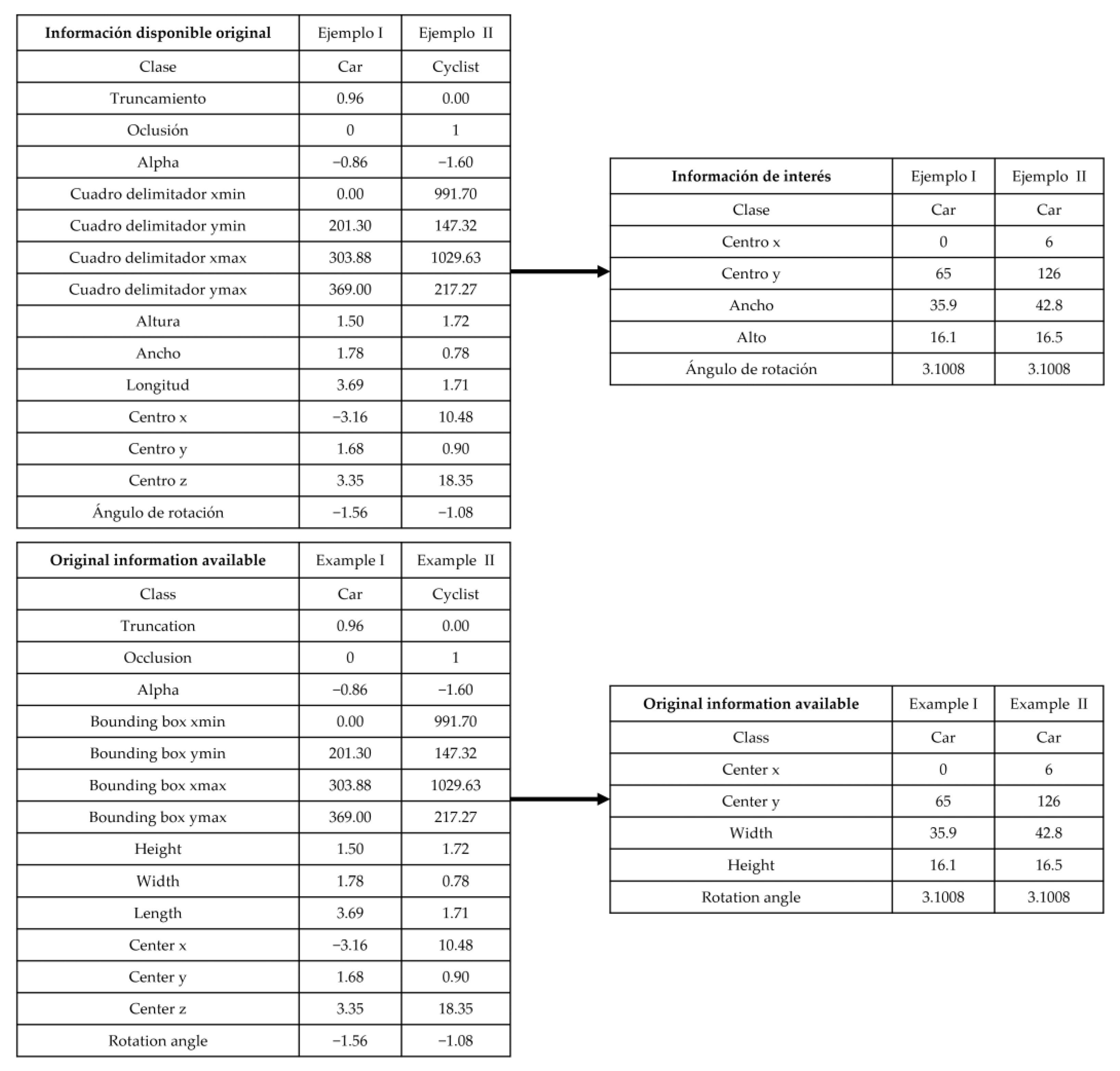
• A step-by-step explanation of the method used during database production, divided into eight sections, with an emphasis on ways of reproducing the process of database creation in order to allow for the possibility of taking different considerations into account when creating any of the three types of formats, such as considering different types of classes or different methods of creating ground-truth segmentation maps.
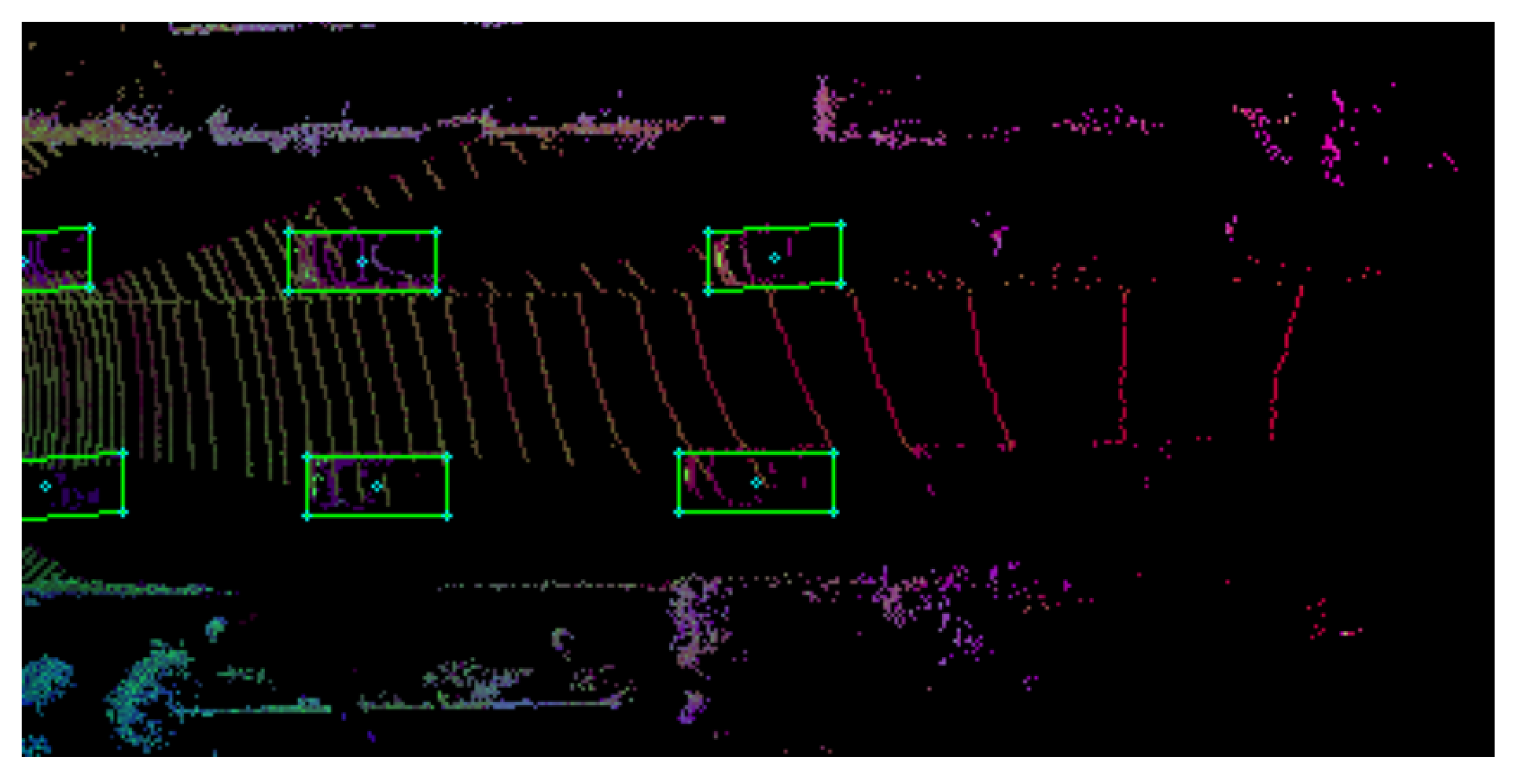
• The creation of a database that includes 7481 top-view segmentation map files of urban scenes, segmenting the road, background, cars, vans, and pickups. These types of files do not exist in other databases, as far as we are aware, and are necessary for environmental perception in autonomous vehicles. In addition, the method of their creation is included, highlighting that the database only has biases during path segmentation because the objects of interest are found through certain mathematical manipulations.
• The results of road segmentation metrics F1-95.77, AP-92.54, ACC-97.53, PRE-94.34, and REC-97.25 are superior to the state-of-the-art.

2. Related Work

2.1. Semantic Segmentation Top-View Works Related to Autonomous Vehicles

Currently, there are works where segmentation analysis is used from top-view scenes as the primary convention of research, which leads to positive results for autonomous vehicle management. Examples of the above can be found in [22], in which a comparison is made between a U-Net and a fully convolutional network (FCN) for the road segmentation task in 2D images of aerial views, where the metrics of each neural network with different image sizes stand out. In the same way, the efficient neural network (ENet) can be used to infer the position and properties of the lines of a highway by segmenting roads in 2D images of aerial maps and generating a grid map that identifies the lateral and central lines of the road, seeking to support autonomous vehicle management with the generation of this information [23]. Another example of this is found in [24], where researchers used 3D scenes acquired with radar to generate 2D top-view maps that they used as input for the fully convolutional neural network, SegNet, and U-Net networks, in an effort to segment the streets, cars, edges, and fences as the output of the network in the 2D top-view plan form.

2.2. LiDAR Semantic Segmentation Top-View Works Related to Autonomous Vehicles

Point cloud scenes from LiDAR sensors are commonly used in conjunction with top-view segmentation maps. In [25], the authors propose, with excellent results in road segmentation, a fully convolutional network that is taken as a basis from which to form three different models that merge the two input scenes differently in each case: one is captured with a LiDAR sensor and the other with an RGB camera. As another example, a new convolutional neural network structure has been designed that outputs a top-view image that segments vehicles and the road from a cloud with a low density of 3D points, taking as input three frontal scenes transformed from the 3D view of a LiDAR [26]. As a further example, in [27], an algorithm is generated that uses some of the segmentation networks proposed and tested to obtain segmented 2D images with the detection of different classes using a simple 2D image of a view of the 3D scene taken with a LiDAR. However, the most crucial previous research in respect of this type of work is the article [28], where the LoDNN neural network is proposed, which is used as a guide for road segmentation from RGB top-view cloud point images. Each point cloud is captured with the LiDAR sensor and transformed into an RGB image by manipulating each captured point’s three-dimensional coordinates (X, Y, Z) and intensity.

In recent research [29,30,31], branches composed of several neural network layers have been proposed and used as a feature extraction block in an artificial intelligence model, demonstrating promising results in the proposed task according to the presented metrics, which outperform previous methods. Such branches can be used in future work to improve the performance of networks such as LoDNN.

2.3. Databases for Autonomous Vehicle Research

There have been several proposals for databases to be created to be used in autonomous driving. In [32], a database was created with synchronized scenes from a LiDAR with 360° and stereo cameras around two cities and under various conditions, providing ground-truth tracking and annotation of 3D objects. This database provides a good reference point for automatic mapping and trajectory detection, such as turning at intersections, driving with many vehicles nearby, and lane changes. In [33], a database was created with more than 1000 h of training data for autonomous vehicles on the same route, generated over five months. This provides high-quality scenes with information on bounding boxes and their class probability. Similarly, in [34], a database was generated with the synchronized capture of data from a LiDAR sensor and a camera, with around 12 million 3D LiDAR and 12 million 2D camera manual box annotations with track identifiers, as well as more than 113 k LiDAR object tracks and 250 k camera image tracks. Like these examples, there are many more databases and sources ofinformation related to autonomous vehicles [35].

2.4. Databases for Autonomous Vehicles with Segmented Scenes

Returning to the databases previously proposed, we identified various studies with respect to segmentation scenes. In [36], a large-scale multimodal database was proposed for autonomous vehicles (AVs) with 360° vision from vision and range sensors such as cameras, lidar, radars, and IMUs. It has 1000 scenes, taken every 20 s, which collect information on various circumstances along its path, providing new metrics for the 3D detection and tracking of 23 object classes with eight attributes for each one. Article [37] presents a database of highly detailed 3D point cloud segmented sequences with 22 identifiable object classes, with 3D scenes based on the line of a moving car. The database in [38] comprises street scenes that present a high degree of segmentation difficulty, with examples of 2D images with their respective segmented 2D maps with up to 25 different classes. In addition, there are point cloud files with separate segmented 3D maps and video frames with instance-level annotations.

2.5. Research in Respect of KITTI Vision Benchmark Dataset

As suggested by the publication and release of the KITTI database, studies on autonomous management that use KITTI have not stopped emerging [20]. One example of this is article [39], in which three models are proposed that use as input the combination of an RGB image of a street scene, with its respective 3D scene generated with a point cloud for two models and the 3D scene converted into a top-view image for the third model. The authors of that study developed 3D detection of the bounding box of the searched objects and classes. The authors of [40] used Yolov3 and the Darknet-53 convolutional neural network to detect cars, trucks, pedestrians, and cyclists on the road using the KITTI database. In [41], the authors designed an algorithm that includes a neural network based on a YOLOv4 network, capable of segmenting objects in a different color and finding a 2D region of interest (ROI). This, in turn, facilitates the detection of objects in 2D camera images.

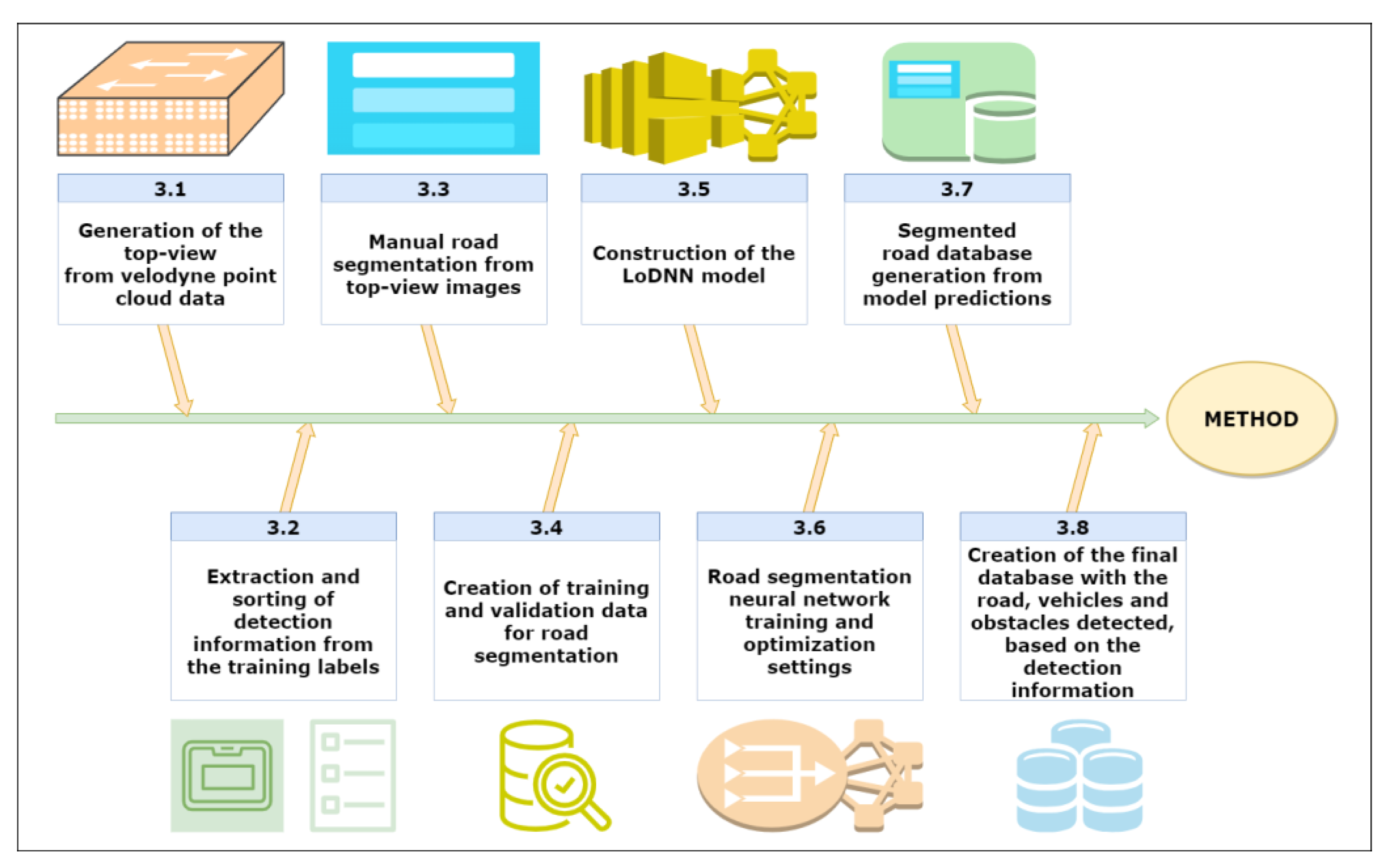
3. Materials and Methods

In this section, the necessary steps are presented to generate the proposed database (Figure 1), which has three parts: 2D top-view image scenes, segmentation map scenes, and the required labels to create each object’s bounding box within each scene.

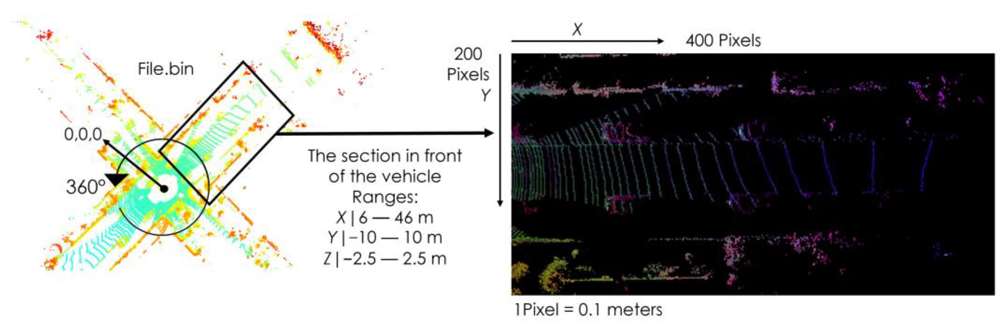
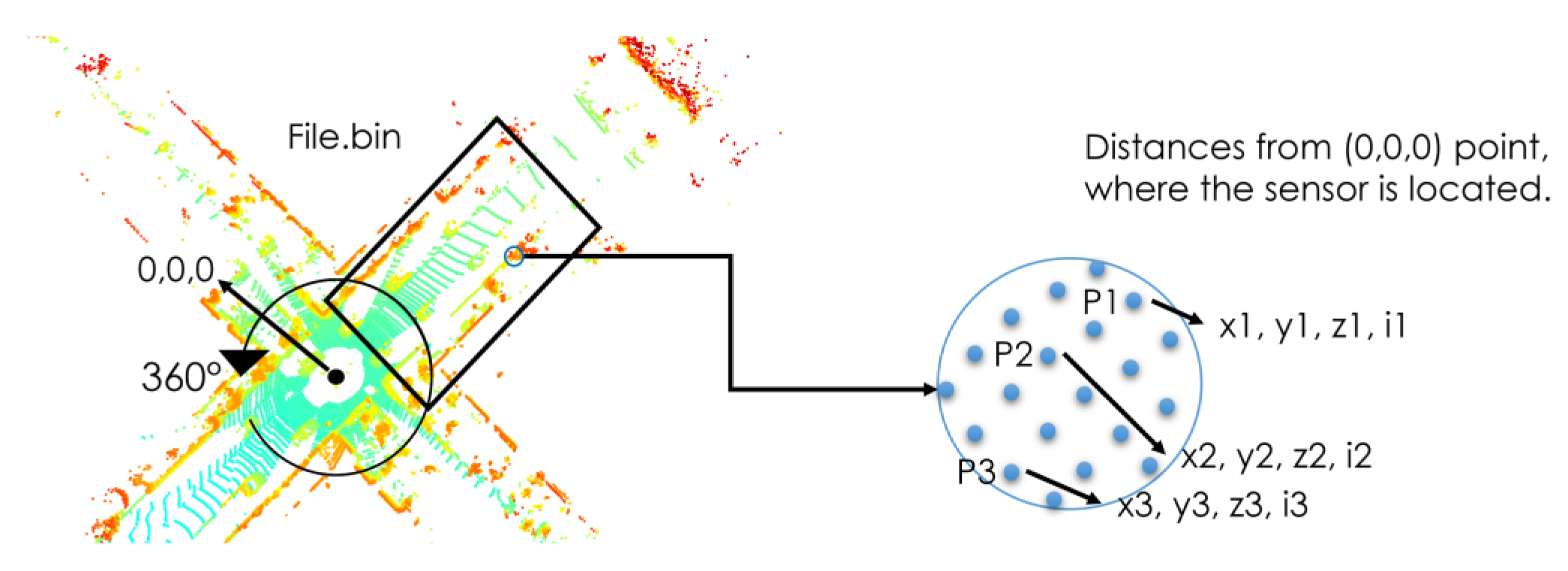
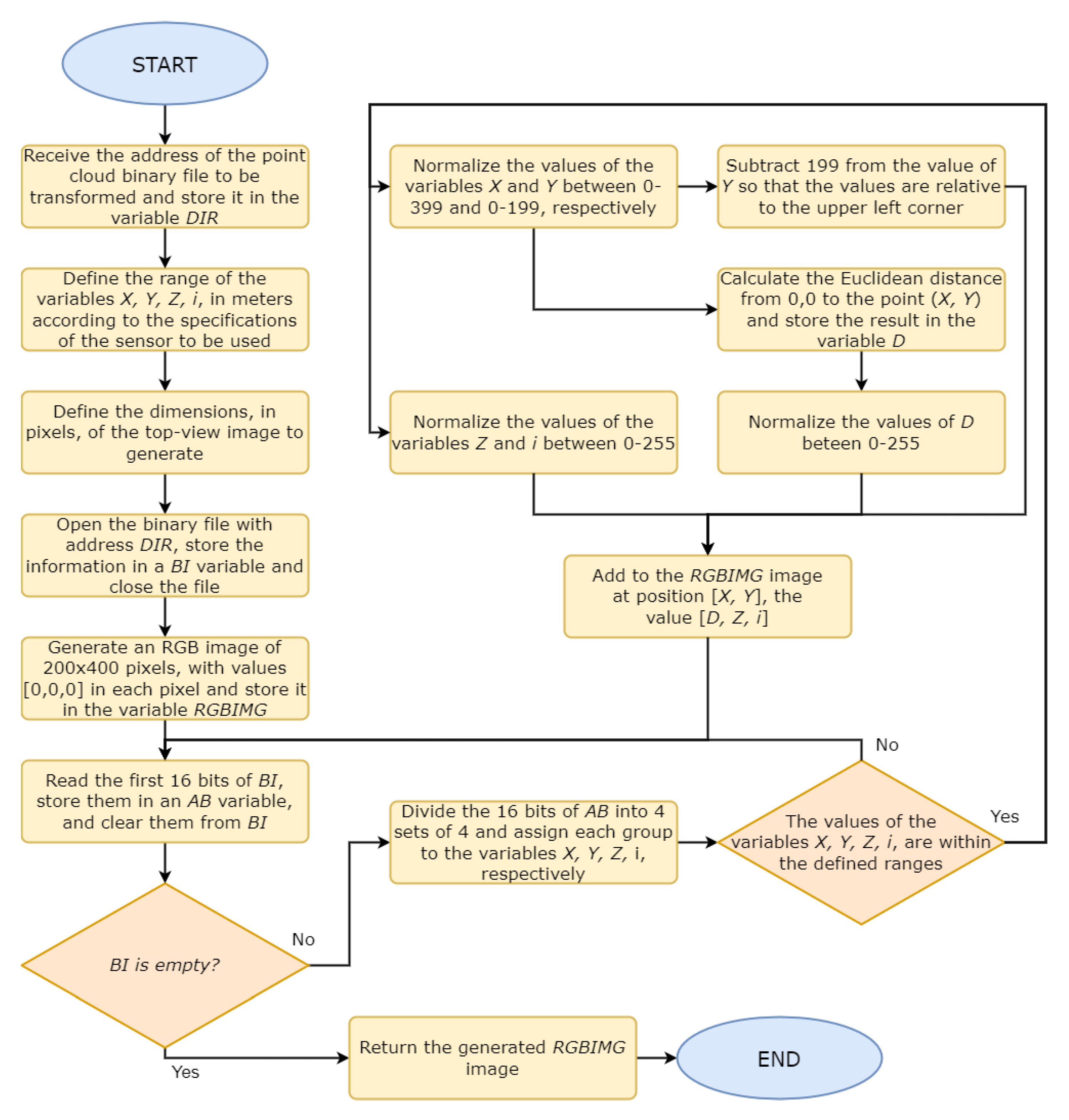
3.1. Generation of the Top-View from the Velodyne Point Cloud Data

The objective of this section is to take the point cloud binary files of each scene from the original database and transform them into the final 2D top-view images (Figure 2) as the first part of the database.

First, it is necessary to understand how the binary files for each scene are structured. As can be seen in Figure 3, each file contains the information of multiple points that make up the so-called three-dimensional point cloud of the scene, 360° around the vehicle that collects the information (test vehicle, TV). For each one of the points, information is obtained on the position of the point in three dimensions (X, Y, Z) concerning the coordinates of the center of the TV (0, 0, 0) and the intensity of light reflected by that point (i).

It is necessary to mention that all the binary files used were obtained from a Velodyne LiDAR sensor; however, this method is compatible with any other brand of LiDAR sensor as long as it is possible to obtain the X, Y, Z, i values of each of the points that make up a scene.

Once the above is understood, the next stage is to determine how a top-view image is generated, 200 × 400 pixels in this case, from the point cloud. Firstly, it is necessary to mention that only the front section of each point cloud scene will be considered, as it is the section of interest for a vehicle moving forward. Then, it must be noted that the LiDAR sensor with which the information is captured will have specific ranges, as shown in Figure 1, in each dimension. In addition, it must be taken into account that the values of the coordinates of each point are provided in meters, and it is proposed to convert each value from meters to pixels, considering that a pixel is equivalent to 0.1 m. In this way, all that remains is to find the value that each pixel will have in the top-view image, for which we need to assign to each point within the range in the point cloud its value in RGB and its position within the image (pixel number), as shown in Figure 3. To find the point’s position, it is necessary to take its X and Y values, convert them to their respective values in pixels and round those values to the nearest whole number, and finally normalize them between 0 and 399 in the case of the X coordinate and 0 and 199 for the Y coordinate. If several points touch the same position, the one with the highest value in its Z coordinate must be considered. Then, in the case of the RGB value that corresponds to each point, its data (X, Y, Z, and i) are deemed to assign in R the value of the distance from the origin (d), which is calculated with the Euclidean distance equation shown in Figure 4; in G the value of Z; and in B the value of i, remembering to convert the values from meters to pixels and to then normalize between 0 and 255 each data point in R, G, and B (d, z, i).

As extra support during the development of this section of the method, the flowchart to transform the point cloud into a top-view image is presented in Figure 5. In addition, a couple of images (Figures S1 and S2) with the pseudocode containing the programming logic suggested for the development of this section are provided in the sup-plementary material of this article.

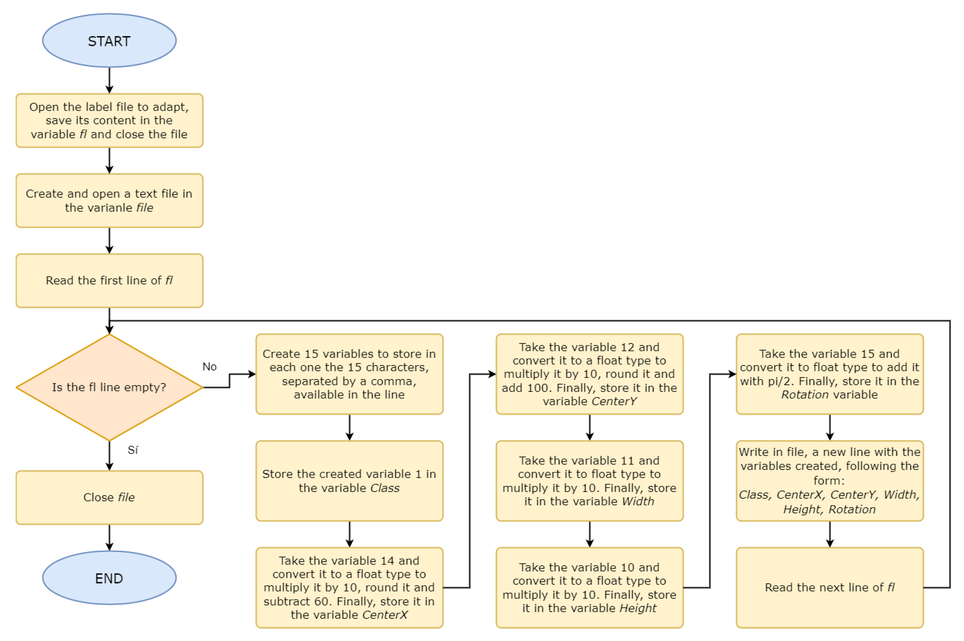
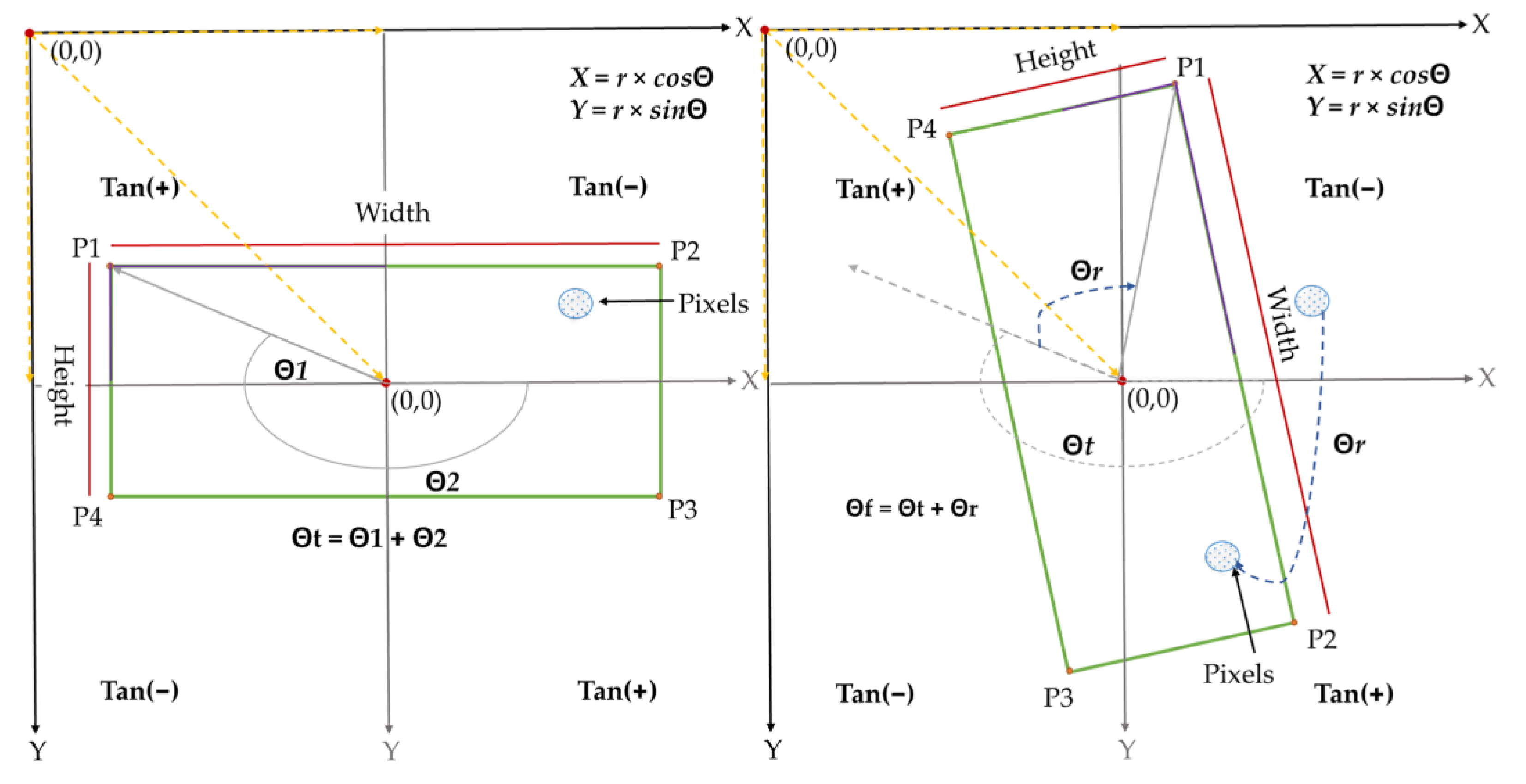
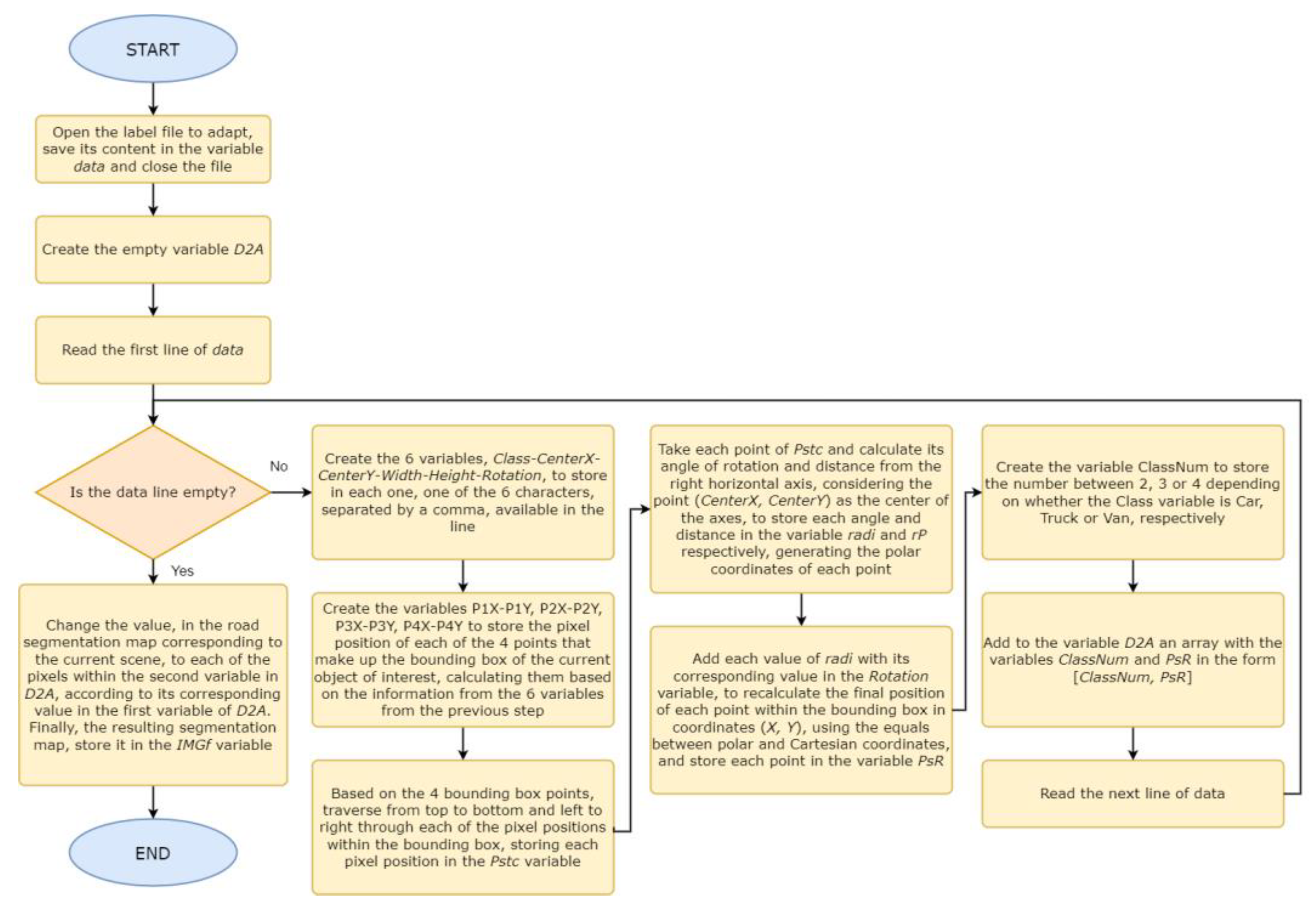
3.2. Extraction and Arrangement of the Detection Information from the Training Labels

In this subsection, we seek to take the labels provided by the KITTI database and select only the information that interests us, as shown in Figure 6. In this case, we seek the information necessary to locate the two-dimensional center of the objects of interest in the top image view, such as its bounding box, achieving the representation of Figure 7, and it is necessary to highlight the fact that in the labels, the origin of the values of the vertical axis is right in the middle of the image. We seek to generate the label files representing the database’s second part. In addition, the original database has various classes in the labels, not all of which may be relevant to the new labels, so we must consider a restriction to only store information on objects of interest.

To achieve the above, it is necessary to locate the exact position number, considering that points are separated by a space, of each of the variables of interest in the original tag files. Then, when opening each file, data are extracted and saved as a temporary variable per file for each of the data of interest per object, locating them according to their position number and storing the temporary variables in the same format as the original file. That is, we separate each variable of interest using spaces and each cluster of per-object variables is separated by a new line. In this way, all that remains is to generate a new file that stores the temporary variable for each original scene.

In the same way as in the previous subsection, a flowchart is provided in Figure 8 to guide the development of this stage and an image (Figure S3) with the pseudocode is provided in the supplementary material.

From the following subsection to Section 3.7, the objective is to generate the road segmentation map in each scene of the generated top-view images.

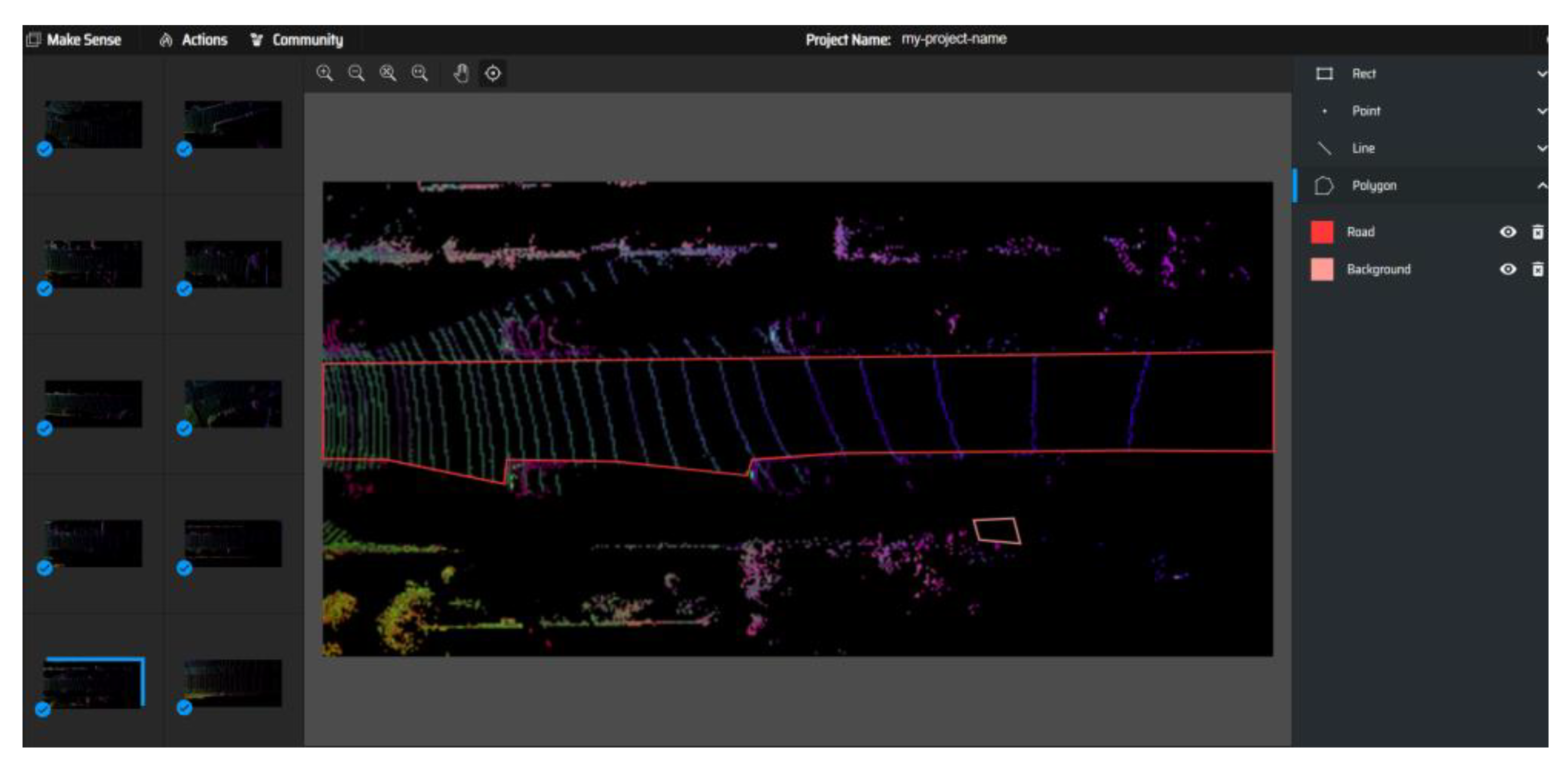
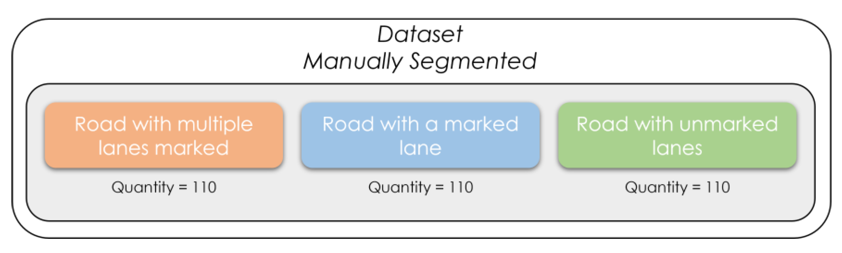
3.3. Manual Road Segmentation from Top-View Images

Firstly, by analyzing each scene of the generated top-view pictures, 100 images are selected with the single-lane road marked, another 100 are selected with the multi-lane road marked, and the last 100 are selected with the road not marked.

In this subsection, we use the selected images to manually segment the road using the MakeSense online software package [42], as shown in Figure 9. In some cases, we use the easily observable figure of the road as a guide, and in others, where the road is not so clear, we find the way by comparing the top-view images with the frontal photos taken with a camera provided as part of the KITTI database [20]. The segmentation carried out with MakeSense is performed through multiple points around each figure considered to be of a particular class; however, it is necessary to take into account that for this specific case, it is only required to create two classes (background and road). It is only necessary to segment the road precisely, while in the case of the background, we only generate a box somewhere outside the section considered a road; this will serve to develop the segmented map of each scene as the ground truth.

It is recommended that the result of the segmentation with the proposed software beobtained as a file in COCO format to generate the segmentation maps later, as shown in Figure 10. This is an image with the exact dimensions of the manually segmented image, in which each pixel is assigned an integer value according to the corresponding class; in this case, either 0 or 1.

Python [43] is recommended to transform the files in COCO format into segmentation maps using the ‘pycocotools.coco’ library. In the programming, it is essential to consider that only the pixels detected as roads are assigned a 1. In contrast, all other pixels are assigned a 0 to enable manual segmentation work, as recommended in the previous subsection.

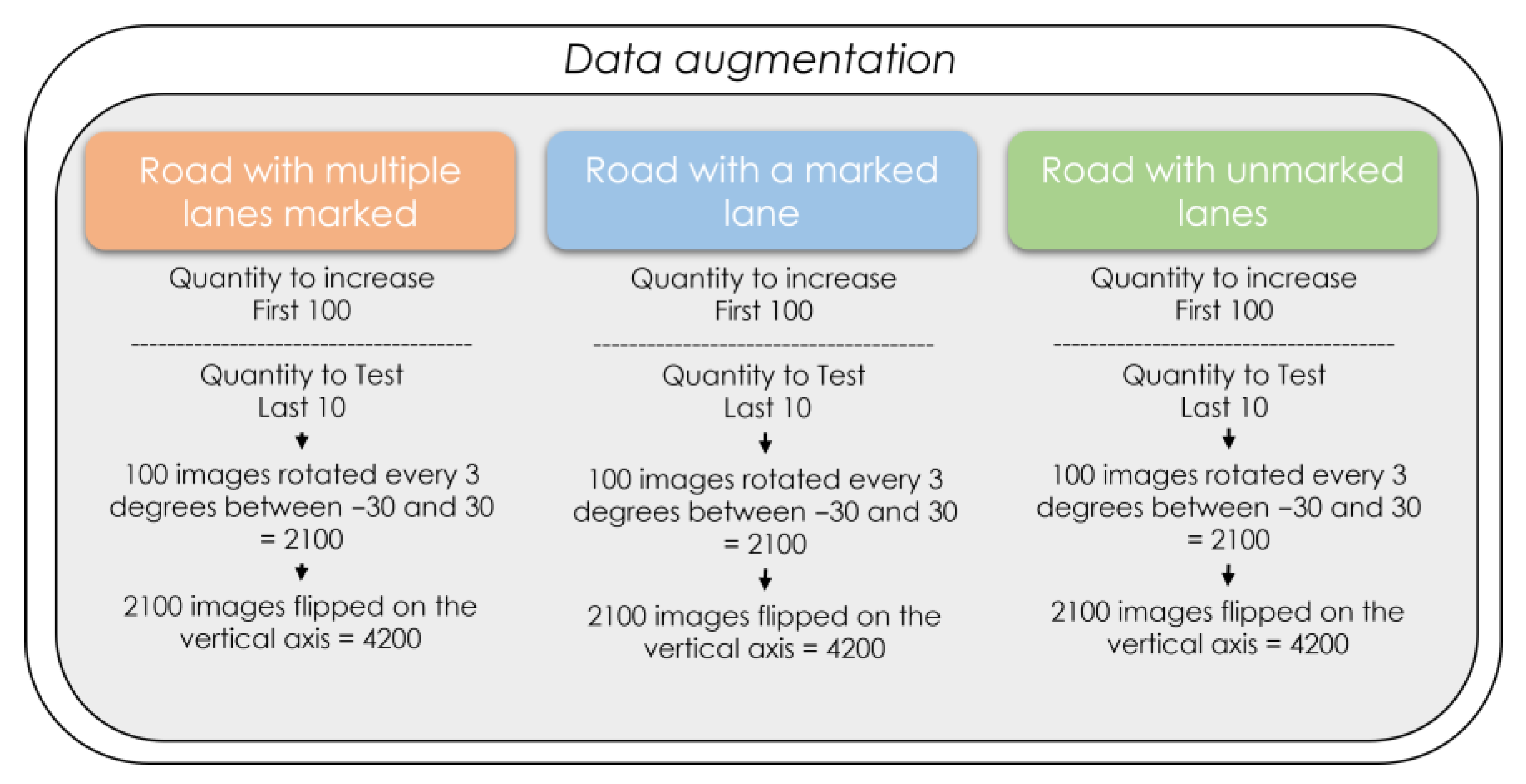
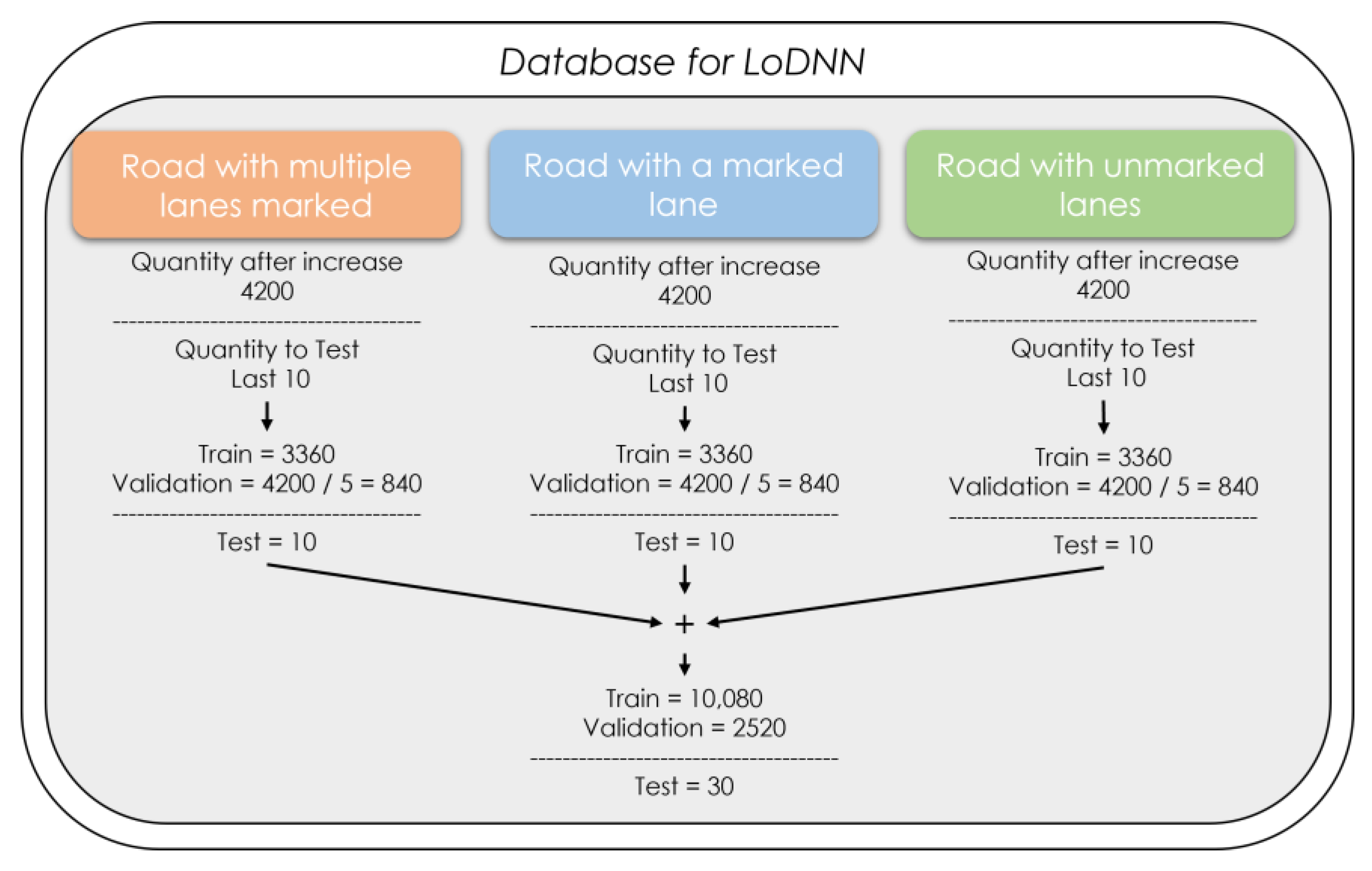
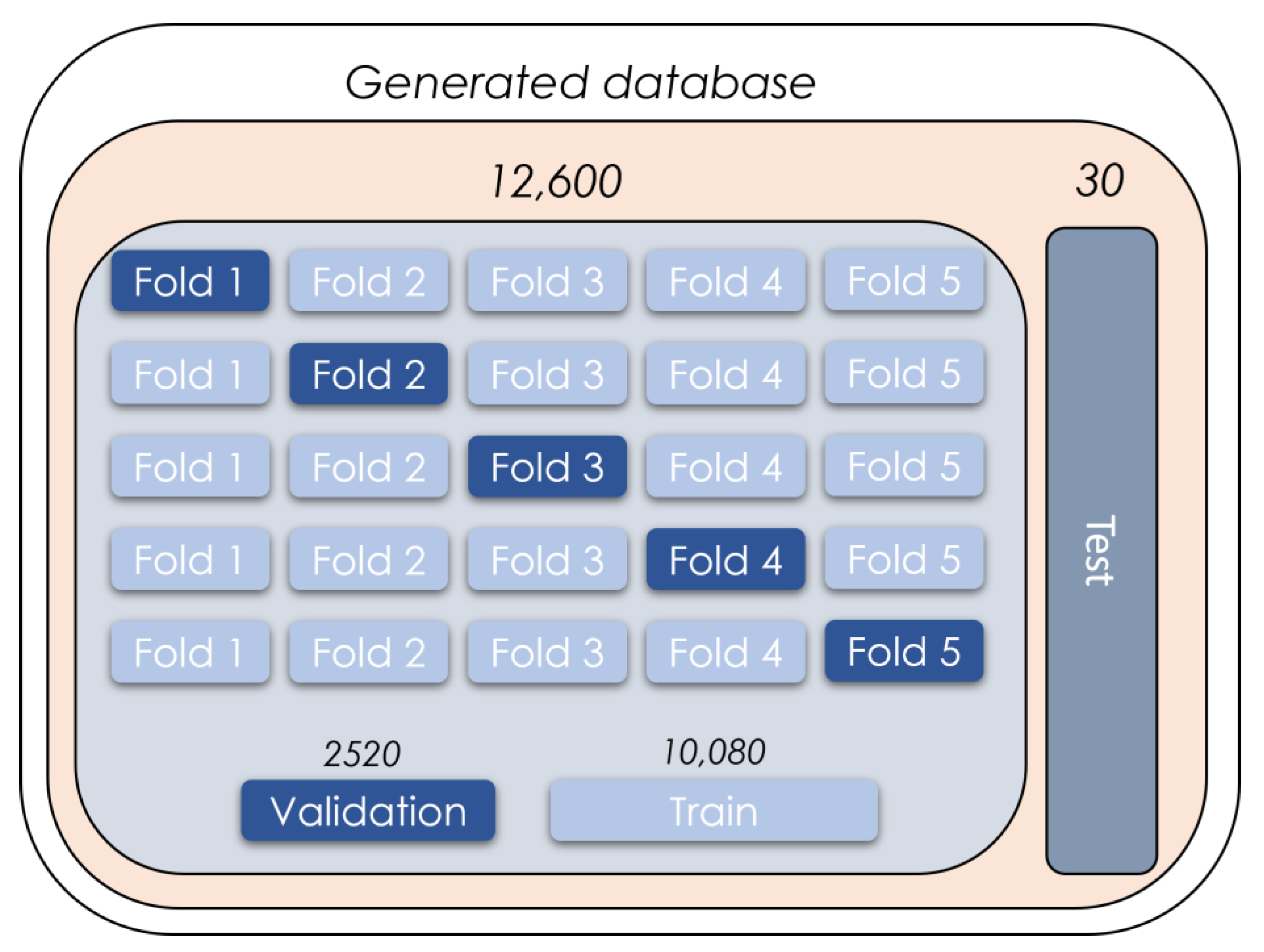
3.4. Creation of Training and Validation Data for Road Segmentation

In this section, each segmentation map created in the last subsection and the top-view images from the first subsection are used to perform data augmentation (see Figure 11), which allows training a model to create a segmentation map of each of the generated top-view scenes.

The data augmentation in respect of both types of scenes (top-view image and segmentation map) follows the instructions in Figure 12.

At the end of the data augmentation procedure, we separate the scene numbers as described in Figure 13, taking together the top-view image and the segmented map of the same scene number.

As the final phase of this subsection, we generate five training databases with different scene numbers for training and validation, as shown in Figure 14, to generate the databases for 5-fold validation.

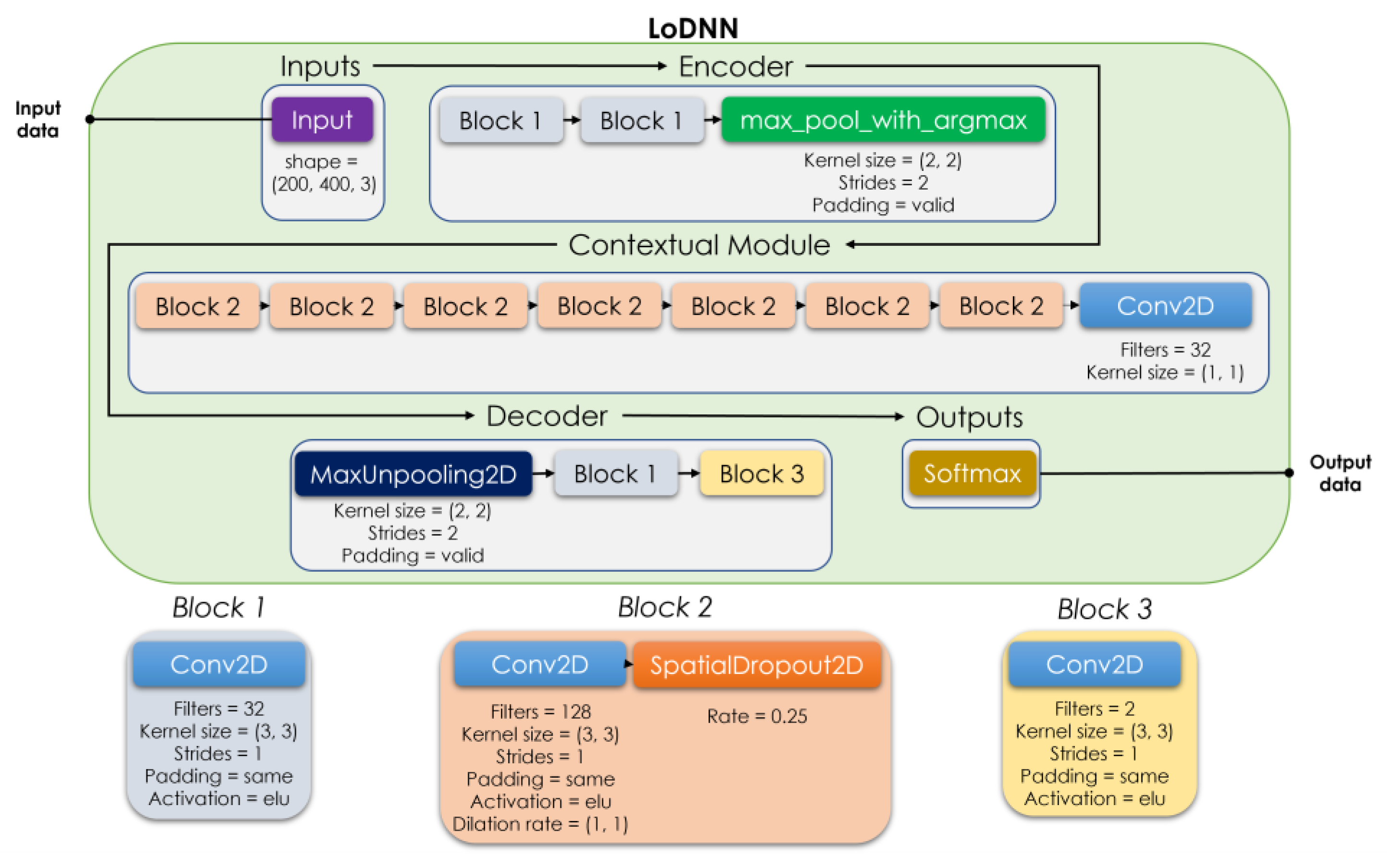
3.5. Construction of the LoDNN Model

Once the database is generated, it is possible to proceed to the generation of the structure of an artificial intelligence model, which, once trained, can infer the road segmentation map of each top-view scene generated in Section 3.1. The suggested design is the LoDNN model proposed in [28], whose exact implementation structure with hyperparameters is presented in Figure 15 with Tensor Flow and Keras.

The structure of the LoDNN model is designed to encode (Encoder) the input top-view images and reduce the size of what is being analyzed, leaving only the most relevant parts of the input. Data then enter a feature extractor block (Contextual Module), where the model learns the most important properties of the input to distinguish between the classes it has to identify. Finally, the model decodes what it has learned (Decoder) and returns everything to its original size to create a segmented map of the input scene as output.

The hyperparameters were modified with respect to those originally proposed in [28], in order to obtain the results faster and with better performance. The ablation experiments that support the final values selected are summarized in Figure 16, which shows the accuracy achieved in different tests with a single type of modified hyperparameter. The upper-left graph shows variations in the learning rate; the upper-right graph shows changes in the number of epochs; and the lower graph shows changes in the batch size. The learning rate graph shows a triangular structure that highlights 1 × 10^−× as the best value. The epoch plot shows an increase up to epoch number 22 but then shows a trend of no major changes, allowing us to opt for 22 epochs as a recommended minimum. Finally, the batch size graph shows that there is no great variation between one value or another, and we can select the highest value for simple visualization purposes during training.

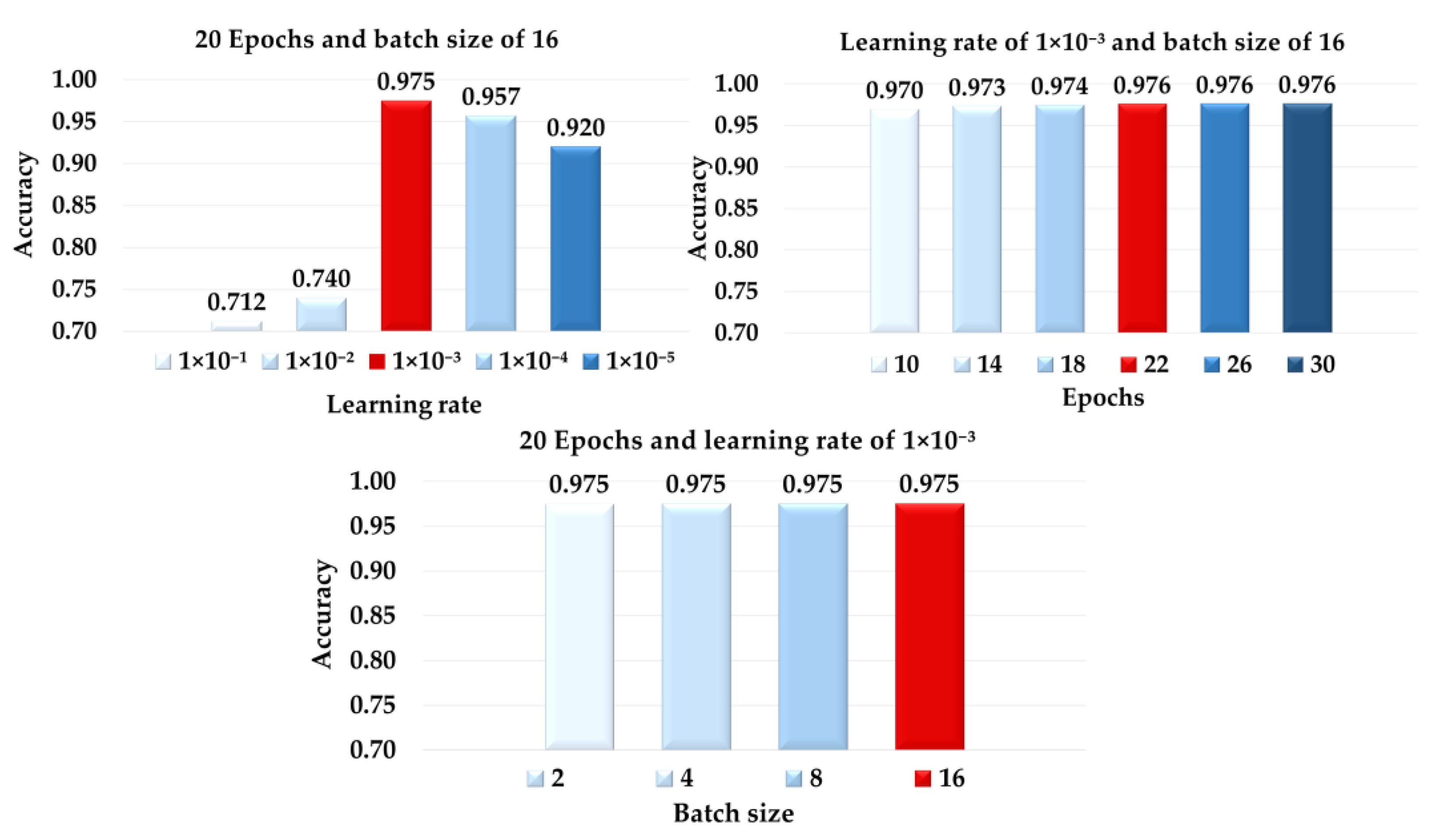
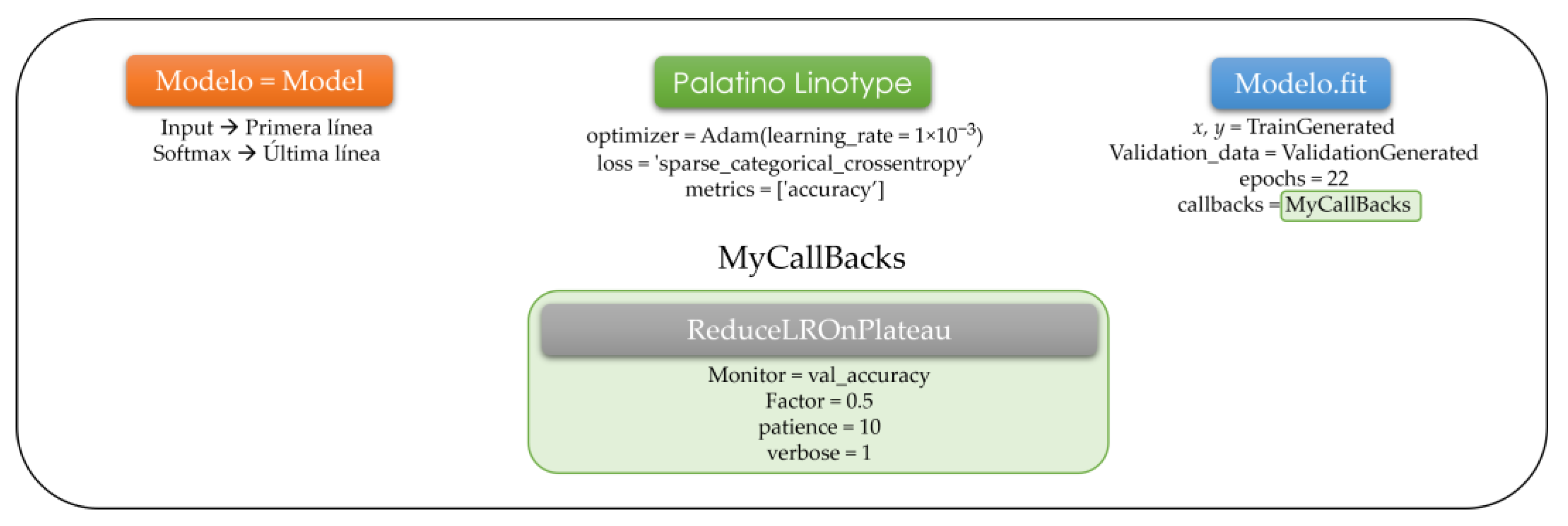
3.6. Training the Neural Network for Road Segmentation and Adjustments for Optimization

In addition to structuring the model, it is necessary to generate, compile, and finally train it, as well as define the hyperparameters of each of these instructions. Following the method in the previous subsection, this procedure is presented in Figure 17. It is necessary to clarify that the data stored in ‘x’ are the matrices of the top-view images normalized between 0 and 1, while the data stored in ‘y’ are the arrays of the segmentation maps of each scene of ‘x’. In the same way, a function is assigned to the callbacks hyperparameter that allows reducing the learning rate during training if a particular chosen metric does not present improvements.

Finally, the model is trained, varying the number of epochs to try to obtain a result with better metrics. In this study, the model was analyzed through tests with 22 epochs, and good results were obtained.

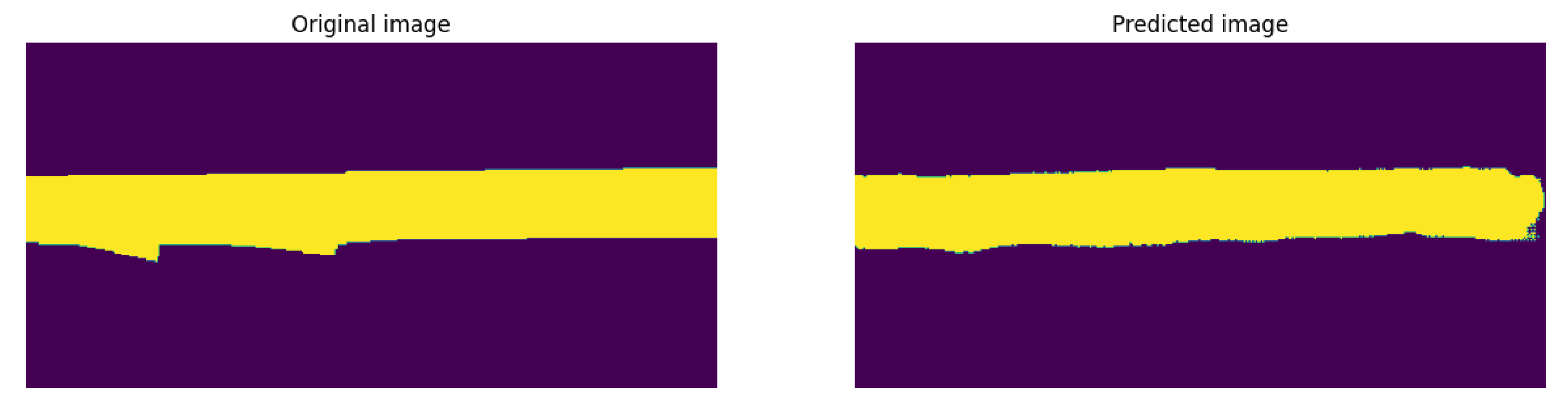
3.7. Generation of the Segmented Road Database from Model Predictions

In this section, the trained model from the previous subsection is used to infer the segmentation map of each of the top-view scenes generated in Section 3.1, as shown in Figure 18. Each of the matrices of the inferred maps is stored in a new variable, which, in this case, we will call ‘Scenes with a segmented path’.

3.8. Creation of the Final Database with the Path, Vehicles, and Obstacles Detected, Taking the Detection Information as a Reference

As a last step, we generate the previous part of the proposed database with segmentation maps that include the objects of interest; in this case, these are background, road, car, van, and truck. To achieve this, each map of the segmented road scenes is taken, and the objects of interest present are added according to the scene number. The number is considered because the labels generated in Section 3.2 will be taken into account, both to determine the number of objects to add in each scene and to understand the corresponding location of the bounding box of each object in the scene. We consider that each pixel within a bounding box will correspond to a specific class, and therefore the value of each of those pixels within the segmentation map will have to be changed to the value corresponding to the class of the object. The proposed object numbers are as follows: background, 0; road, 1; car, 2; van, 3; and truck, 4.

As a method of generating a bounding box, we first propose to generate it without taking rotation into account in order to identify each of the pixels within the generated rectangle and to later rotate them by a certain angle indicated in the file of labels in radians. In addition, both images in Figure 19 show the mathematical considerations necessary to determine the position in two-dimensional coordinates of each of the points within the unrotated bounding box (all points within the four corners of the bounding box) and to subsequently calculate the variables t and r of each point according to the conversion formulas between polar and Cartesian coordinates. We finally rotate each of the points, considering that the angle in the label file is only the angle r and the final angle of each point is actually f. It is recommended that the values of the vertical axis are changed so that the origin is at the top, resulting in the values of the centers of each object being based on the 0,0 coordinate of the upper-left corner of the segmentation map.

As in the previous sections, a flowchart is presented in Figure 20 for carrying out this final stage of the proposed methodological process to support the understanding and possible duplication of this work. Similarly, five images (Figures S4–S8) with the pseu-docode containing the suggested programming logic for this stage are provided in the supplementary material.

4. Results

As the first result of the general method described, road segmentation scenes were created. These are referred to as LoDNN-I (LiDAR-only deep neural network—improved). This system allows result metrics such as those in

Table 1. Road segmentation results metrics pertaining to the test set.

Method	F1	AP	ACC	PRE	REC
LoDNN-I (proposal)	95.77	92.54	97.53	94.34	97.25

and the confusion matrix in Figure 21 to be obtained.

Then, based on the created road segmentation scenes, a segmentation map was mathematically created for each scene (Figure 22), along with each top-view point cloud image and its 2D label file. An image containing the information from the three sections included in the proposed database is presented in Figure 23.

5. Discussion

In this paper, we have presented a database with top-view images, segmentation maps, and labels of the positions of the objects of interest. We have also described the method by which it was created and the development of a database with different considerations. Using this, a set of segmentation maps of top-view images of point clouds was created. This cluster is not state-of-the-art as far as we are aware. A significant advantage of the method proposed during the creation of the segmentation maps is that it will allow matching the segmentation of each object of interest with its respective detection label. In addition, the road segmentation in each scene presents high performance in comparison with similar, fairly recent state-of-the-art methods, according to the test dataset metrics (

Table 2. Comparison of the result metrics obtained in this study with those used in other road segmentation works, adapted from [25].

Methods	F1	AP	PRE	REC
LoDNN-I (proposal)	95.77	92.54	94.34	97.25
LoDNN [28]	94.07	92.03	92.81	95.37
Up-Conv-Poly [44]	93.83	90.47	94.00	93.67
DDN [45]	93.43	89.67	95.09	91.82
FTP [46]	91.61	90.96	91.04	92.2
FCN-LC [47]	90.79	85.83	90.87	90.72
HIM [48]	90.64	81.42	91.62	89.68
NNP [49]	89.68	86.5	89.67	89.68
RES3D-Velo [50]	86.58	78.34	82.63	90.92

). Good results are obtained with LoDNN-I compared to other research that utilizes the LoDNN model; this is the same neural network used for the same objective but with a different ground truth generation methodology. In addition, how the neural network structure for road segmentation should be built was presented directly in this paper, including the necessary considerations during its programming with the proposed libraries, to save time during the reproduction of this work or the creation of a neural network in general for some other work. Specifically, this database will be used in research on autonomous vehicle perception, in which top-view images are used as input to a neural network, and segmentation maps in conjunction with labels are used as the ground truth for training.

Among the limitations of this work, the proposed database was explicitly created for use with a top-view point cloud, which limits the types of applications in which it can be used. In addition, during the development of the general method presented herein, the database is focused on detecting only three objects (vehicles) of the seven well-identified available objects. Another limitation is that the database only considers objects detectable by LiDAR sensors. However, in future research, we propose an alternative of integrating several sensors into the same system in order to enrich the information obtained during the data acquisition. The method is also limited by using information from only one LiDAR sensor, so in future work, it is proposed that part of the proposed method is used to generate independent LiDAR databases that can be used to reconstruct scenes formed by point clouds. The last limitation of this work is time; if more time was available, an integrated system could be implemented in a vehicle to collect new scenes and expand the database, placing the LiDAR sensor in the same position as suggested by the researchers who created the KITTI database.

6. Conclusions

In this paper, a method was described, in eight subsections, for the elaboration of a database consisting of 7481 scenes, each represented by three types of files (top-view point cloud images, two-dimensional segmentation maps, and in-plane labels of position, dimensions, and rotation) for each of the three types of vehicles detected in each scene. When creating top-view images, some points overlap at the same position of a pixel. In these cases, using the highest point to define a value as the final value of that pixel is sufficient for convolutional neural network models to find features to segment and detect objects. However, when generating ground-truth segmentation maps, taking as a reference the road guidelines clearly visible in the top-view images allows functional and simple manual segmentation using software, which in turn makes it possible for a convolutional neural network to improve its performance during the inference of new segmentation maps.

The main contribution of this study is the proposal for creating top-view segmentation maps of urban scenes, whose data type does not exist in other databases, and this is necessary for environmental perception work in respect of autonomous vehicles. With this proposal, road segmentation metrics in respect of F1-95.77, AP-92.54, ACC-97.53, PRE-94.34, and REC-97.25 can be obtained. In addition, thanks to the proposed method, only road inference bias exists in the segmentation maps created, since the rest of the segmented classes were added through mathematical manipulations that allowed them to precisely match each vehicle’s segmentation within the scene with their respective labels in the plane.

References

1. Yurtsever, E.; Lambert, J.; Carballo, A.; Takeda, K. A Survey of Autonomous Driving: Common Practices and Emerging Technologies. IEEE Access 2020, 8, 58443–58469. [Google Scholar] [CrossRef]
2. Society of Automotive Engineers International. Taxonomy and Definitions for Terms Related to Driving Automation Systems for On-road Motor Vehicles; SAE International: Warrendale, PA, USA, 2018; pp. 1–35. [Google Scholar]
3. National Highway Traffic Safety Administration. Automated Driving Systems 2.0: A Vision for Safety; National Highway Traffic Safety Administration: Washington, DC, USA, 2017. [Google Scholar]
4. Bachute, M.R.; Subhedar, J.M. Autonomous Driving Architectures: Insights of Machine Learning and Deep Learning Algorithms. Mach. Learn. Appl. 2021, 6, 100164. [Google Scholar] [CrossRef]
5. Dewangan, D.K.; Sahu, S.P. RCNet: Road classification convolutional neural networks for intelligent vehicle system. Intell. Serv. Robot. 2021, 14, 199–214. [Google Scholar] [CrossRef]
6. Gkolias, K.; Vlahogianni, E.I. Convolutional Neural Networks for On-Street Parking Space Detection in Urban Networks. IEEE Trans. Intell. Transp. Syst. 2019, 20, 4318–4327. [Google Scholar] [CrossRef]
7. Chen, L.; Lin, S.; Lu, X.; Cao, D.; Wu, H.; Guo, C.; Liu, C.; Wang, F.-Y. Deep Neural Network Based Vehicle and Pedestrian Detection for Autonomous Driving: A Survey. IEEE Trans. Intell. Transp. Syst. 2021, 22, 3234–3246. [Google Scholar] [CrossRef]
8. Song, W.; Zou, S.; Tian, Y.; Fong, S.; Cho, K. Classifying 3D objects in LiDAR point clouds with a back-propagation neural network. Hum.-Cent. Comput. Inf. Sci. 2018, 8, 29. [Google Scholar] [CrossRef] [Green Version]
9. Lu, W.; Zhou, Y.; Whan, G.; Hou, S.; Song, S. L3-Net: Towards Learning Based Lidar Localization for Autonomous Driving. In Proceedings of the 2019 IEEE/CVF Conference on Computer Vision and Pattern Recognition (CVPR), Long Beach, CA, USA, 15–20 June 2019; pp. 6382–6391. [Google Scholar]
10. Wu, B.; Wan, A.; Yue, X.; Keutzer, K. SqueezeSeg: Convolutional Neural Nets with Recurrent CRF for Real-Time Road-Object Segmentation from 3D LiDAR Point Cloud. In Proceedings of the IEEE International Conference on Robotics and Automation, Brisbane, Australia, 21–25 May 2018; pp. 1887–1893. [Google Scholar]
11. Chen, B.; Gong, C.; Yang, J. Importance-Aware Semantic Segmentation for Autonomous Vehicles. IEEE Trans. Intell. Transp. Syst. 2019, 20, 137–148. [Google Scholar] [CrossRef]
12. Wang, Y.; Wang, L.; Hu, Y.H.; Qiu, J. RailNet: A Segmentation Network for Railroad Detection. IEEE Access 2019, 7, 143772–143779. [Google Scholar] [CrossRef]
13. Lyu, Y.; Bai, L.; Huang, X. Road segmentation using CNN and distributed LSTM. In Proceedings of the IEEE International Symposium on Circuits and Systems, Sapporo, Japan, 26–29 May 2019; pp. 1–5. [Google Scholar]
14. Xia, X.; Meng, Z.; Han, X.; Li, H.; Tsukiji, T.; Xu, R.; Zheng, Z.; Ma, J. An automated driving systems data acquisition and analytics platform. Transp. Res. Part C 2023, 151, 104120. [Google Scholar] [CrossRef]
15. Liu, W.; Xia, X.; Xiong, L.; Lu, Y.; Gao, L.; Yu, Z. Automated Vehicle Sideslip Angle Estimation Considering Signal Measurement Characteristic. IEEE Sens. J. 2021, 21, 21675–21687. [Google Scholar] [CrossRef]
16. Xia, X.; Hashemi, E.; Xiong, L.; Khajepour, A. Autonomous Vehicle Kinematics and Dynamics Synthesis for Sideslip Angle Estimation Based on Consensus Kalman Filter. IEEE Trans. Control Syst. Technol. 2023, 31, 179–192. [Google Scholar] [CrossRef]
17. Yang, D.; Li, L.; Redmill, K.; Ozguner, U. Top-view trajectories: A pedestrian dataset of vehicle-crowd interaction from controlled experiments and crowded campus. In Proceedings of the IEEE Intelligent Vehicles Symposium, Paris, France, 9–12 June 2019; pp. 899–904. [Google Scholar]
18. Azimi, S.M.; Fischer, P.; Korner, M.; Reinartz, P. Aerial LaneNet: Lane-Marking Semantic Segmentation in Aerial Imagery Using Wavelet-Enhanced Cost-Sensitive Symmetric Fully Convolutional Neural Networks. IEEE Trans. Geosci. Remote Sens. 2019, 57, 2920–2938. [Google Scholar] [CrossRef] [Green Version]
19. Pek, C.; Manzinger, S.; Koschi, M.; Althoff, M. Using online verification to prevent autonomous vehicles from causing accidents. Nat. Mach. Intell. 2020, 2, 518–528. [Google Scholar] [CrossRef]
20. The KITTI Vision Benchmark Suite. Available online: http://www.cvlibs.net/datasets/kitti/eval_object.php?obj_benchmark=bev (accessed on 22 February 2023).
21. Geiger, A.; Lenz, P.; Urtasun, R. Are we ready for Autonomous Driving? The KITTI Vision Benchmark Suite. In Proceedings of the IEEE Computer Society Conference on Computer Vision and Pattern Recognition, Providence, RI, USA, 16–21 June 2012; pp. 3354–3361. [Google Scholar]
22. Ozturk, O.; Saritürk, B.; Seker, D.Z. Comparison of Fully Convolutional Networks (FCN) and U-Net for Road Segmentation from High Resolution Imageries. Int. J. Environ. Geoinform 2020, 7, 272–279. [Google Scholar] [CrossRef]
23. Carneiro, R.V.; Nascimento, R.C.; Guidolini, R.; Cardoso, V.B.; Oliveira-Santos, T.; Badue, C.; De Souza, A.F. Mapping Road Lanes Using Laser Remission and Deep Neural Networks. In Proceedings of the International Joint Conference on Neural Networks, Rio de Janeiro, Brazil, 8–13 July 2018; pp. 1–8. [Google Scholar]
24. Prophet, R.; Li, G.; Sturm, C.; Vossiek, M. Semantic segmentation on automotive radar maps. In Proceedings of the IEEE Intelligent Vehicles Symposium, Paris, France, 9–12 June 2019; pp. 756–763. [Google Scholar]
25. Caltagirone, L.; Bellone, M.; Svensson, L.; Wahde, M. LIDAR–camera fusion for road detection using fully convolutional neural networks. Robot. Auton. Syst. 2019, 111, 125–131. [Google Scholar] [CrossRef] [Green Version]
26. Lee, J.S.; Jo, J.H.; Park, T.H. Segmentation of Vehicles and Roads by a Low-Channel Lidar. IEEE Trans. Intell. Transp. Syst. 2019, 20, 4251–4256. [Google Scholar] [CrossRef]
27. Boulch, A.; Le Saux, B.; Audebert, N. Unstructured point cloud semantic labeling using deep segmentation networks. In Proceedings of the Eurographics Workshop on 3D Object Retrieval, EG 3DOR, Lyon, France, 23–24 April 2017; pp. 17–24. [Google Scholar]
28. Caltagirone, L.; Scheidegger, S.; Svensson, L.; Wahde, M.F. Fast LIDAR-based road detection using fully convolutional neural networks. In Proceedings of the IEEE Intelligent Vehicles Symposium, Los Angeles, CA, USA, 11–14 June 2017; pp. 1019–1024. [Google Scholar]
29. Zhang, W.; Sun, X.; Zhou, L.; Xie, X.; Zhao, W.; Liang, Z.; Zhuang, P. Dual-branch collaborative learning network for crop disease identification. Front. Plant Sci. 2023, 14, 1117478. [Google Scholar] [CrossRef]
30. Zhao, W.; Li, C.; Zhang, W.; Yang, L.; Zhuang, P.; Li, L.; Fan, K.; Yang, H. Embedding Global Contrastive and Local Location in Self-Supervised Learning. IEEE Trans. Circuits Syst. Video Technol. 2023, 33, 2275–2289. [Google Scholar] [CrossRef]
31. Zhang, W.; Li, Z.; Sun, H.; Zhang, Q.; Zhuang, P. SSTNet: Spatial, Spectral, and Texture Aware Attention Network Using Hyperspectral Image for Corn Variety Identification. IEEE Geosci. Remote Sens. Lett. 2022, 19, 1–5. [Google Scholar] [CrossRef]
32. Chang, M.F.; Lambert, J.; Sangkloy, P.; Singh, J.; Bak, S.; Hartnett, A.; Wang, D.; Carr, P.; Lucey, S.; Ramanan, D.; et al. Argoverse: 3D tracking and forecasting with rich maps. In Proceedings of the IEEE Computer Society Conference on Computer Vision and Pattern Recognition, Long Beach, CA, USA, 15–20 June 2019; pp. 8740–8749. [Google Scholar]
33. Mandal, S.; Biswas, S.; Balas, V.E.; Shaw, R.N.; Ghosh, A. Motion Prediction for Autonomous Vehicles from Lyft Dataset using Deep Learning. In Proceedings of the 2020 IEEE 5th International Conference on Computing Communication and Automation, ICCCA 2020, Greater Noida, India, 30–31 October 2020; pp. 768–773. [Google Scholar]
34. Sun, P.; Kretzschmar, H.; Dotiwalla, X.; Chouard, A.; Patnaik, V.; Tsui, P.; Guo, J.; Zhou, Y.; Chai, Y.; Caine, B.; et al. Scalability in Perception for Autonomous Driving: Waymo Open Dataset. In Proceedings of the IEEE/CVF Conference on Computer Vision and Pattern Recognition, Seattle, WA, USA, 13–19 June 2020; pp. 2443–2451. [Google Scholar]
35. Janai, J.; Güney, F.; Behl, A.; Geiger, A. Computer Vision for Autonomous Vehicles: Problems, Datasets and State of the Art; Foundations and Trends® in Computer Graphics and Vision; Now Publishers Inc.: Hanover, MD, USA, 2020; Volume 12, pp. 1–308. [Google Scholar]
36. Caesar, H.; Bankiti, V.; Lang, A.H.; Vora, S.; Liong, V.E.; Xu, Q.; Krishnan, A.; Pan, Y.; Baldan, G.; Beijbom, O. Nuscenes: A multimodal dataset for autonomous driving. In Proceedings of the IEEE Computer Society Conference on Computer Vision and Pattern Recognition, Seattle, WA, USA, 14–19 June 2020; pp. 11618–11628. [Google Scholar]
37. Behley, J.; Garbade, M.; Milioto, A.; Quenzel, J.; Behnke, S.; Stachniss, C.; Gall, J. SemanticKITTI: A Dataset for Semantic Scene Understanding of LiDAR Sequences. arXiv 2019, arXiv:1904.01416. [Google Scholar]
38. Huang, X.; Cheng, X.; Geng, Q.; Cao, B.; Zhou, D.; Wang, P.; Lin, Y.; Yang, R. The apolloscape dataset for autonomous driving. In Proceedings of the IEEE Computer Society Conference on Computer Vision and Pattern Recognition Workshops, Salt Lake City, UT, USA, 18–22 June 2018; pp. 1067–1073. [Google Scholar]
39. Wen, L.H.; Jo, K.H. Fast and Accurate 3D Object Detection for Lidar-Camera-Based Autonomous Vehicles Using One Shared Voxel-Based Backbone. IEEE Access 2021, 9, 22080–22089. [Google Scholar] [CrossRef]
40. Al-refai, G.; Al-refai, M. Road object detection using Yolov3 and Kitti dataset. Int. J. Adv. Comput. Sci. Appl. 2020, 11, 48–53. [Google Scholar] [CrossRef]
41. Fan, Y.C.; Yelamandala, C.M.; Chen, T.W.; Huang, C.J. Real-Time Object Detection for LiDAR Based on LS-R-YOLOv4 Neural Network. J. Sens. 2021, 2021, 11. [Google Scholar] [CrossRef]
42. Make Sense. Available online: https://www.makesense.ai/ (accessed on 26 May 2023).
43. Welcome to Python. Available online: https://www.python.org/ (accessed on 9 March 2023).
44. Oliveira, G.L.; Burgard, W.; Brox, T. Efficient deep models for monocular road segmentation. In Proceedings of the IEEE International Conference on Intelligent Robots and Systems, Daejeon, Republic of Korea, 9–14 October 2016; pp. 4885–4891. [Google Scholar]
45. Mohan, R. Deep Deconvolutional Networks for Scene Parsing. arXiv 2014, arXiv:1411.4101. [Google Scholar]
46. Laddha, A.; Kocamaz, M.K.; Navarro-Serment, L.E.; Hebert, M. Map-supervised road detection. In Proceedings of the IEEE Intelligent Vehicles Symposium, Gothenburg, Sweden, 19–22 June 2016; pp. 118–123. [Google Scholar]
47. Mendes, C.; Frémont, V.; Wolf, D. Exploiting fully convolutional neural networks for fast road detection. In Proceedings of the 2016 IEEE International Conference on Robotics and Automation, Stockholm, Sweden, 16–21 May 2016; pp. 3174–3179. [Google Scholar]
48. Munoz, D.; Bagnell, J.A.; Hebert, M. Stacked Hierarchical Labeling. In Computer Vision—Eccv 2010, Pt Vi; Springer: Berlin/Heidelberg, Germany, 2010; Volume 6316, pp. 57–70. [Google Scholar]
49. Chen, X.; Kundu, K.; Zhu, Y.; Berneshawi, A.; Ma, H.; Fidler, S.; Urtasun, R. 3D object proposals for accurate object class detection. Adv. Neural Inf. Process. Syst. 2015, 2015, 424–432. [Google Scholar]
50. Patrick, Y.; Shinzato, D.F.W.; Stiller, C. Road Terrain Detection: Avoiding Common Obstacle Detection Assumptions Using Sensor Fusion. In Proceedings of the 2014 IEEE Intelligent Vehicles Symposium Proceedings, Dearborn, MI, USA, 8–11 June 2014; pp. 687–692. [Google Scholar]
Figure 1. General diagram of the method proposed for the generation of the database.
Electronics 12 03165 g001
Figure 2. Example of a point cloud scene with the section to be generated as an approximate top-view highlighted on the left and its respective final top-view scene, where each pixel corresponds to 0.1 m, highlighting the ranges in which the points are considered.
Electronics 12 03165 g002
Figure 3. Sample of a scene that can be created from a point cloud binary file, with an approach to a section of points, highlighting the available information for each.
Electronics 12 03165 g003
Figure 4. Summary of the transition between X, Y, Z, and i data for each point in the point cloud within the range, towards a position; RGB values are necessary to form the top-view image of the scene.
Electronics 12 03165 g004
Figure 5. Flowchart to transform a binary point-cloud file into a top-view image.
Electronics 12 03165 g005
Figure 6. KITTI database [20] labels are shown on the left, and the respective labels are already reduced with the objects and values of interest on the right.
Electronics 12 03165 g006
Figure 7. Top-view image generated in the previous subsection with the 2D center (blue *) and bounding box (green rectangle) of each object of interest highlighted.
Electronics 12 03165 g007
Figure 8. Flowchart used to generate a new file with the variables of the objects of interest from a file containing the original labels.
Electronics 12 03165 g008
Figure 9. Example of a manually segmented image using MakeSense online software [42].
Electronics 12 03165 g009
Figure 10. Example of road segmentation map.
Electronics 12 03165 g010
Figure 11. Composition of the dataset with the scenes segmented manually.
Electronics 12 03165 g011
Figure 12. General description of the procedure for data augmentation, noting that test data must be separated before the process.
Electronics 12 03165 g012
Figure 13. Description of the division of generated scenes because of the creation of training, validation, and test data.
Electronics 12 03165 g013
Figure 14. Graphic description of each case’s training and validation data division, performed to obtain five different databases for 5-fold validation.
Electronics 12 03165 g014
Figure 15. Graphical description of the structure of the LoDNN model, with each of the layers in the correct order and their corresponding hyperparameters.
Electronics 12 03165 g015
Figure 16. Graphical summary of the ablation experiments performed to select the best hyperparameters to be used during the training of the LoDNN model.
Electronics 12 03165 g016
Figure 17. Graphical representation of the commands necessary to generate, prepare, and train the model and their corresponding hyperparameters. The name ‘Model’ is given to the developed neural network.
Electronics 12 03165 g017
Figure 18. Example of original and inferred segmentation maps using the LoDNN model with the proposed hyperparameters, where yellow represents the road and purple the background.
Electronics 12 03165 g018
Figure 19. Graphical method for the proposal to generate a bounding box. The image on the left depicts graphically the result of generating a bounding box of an object to be detected in a scene without considering its rotation, while the image on the right shows the same bounding box already rotated.
Electronics 12 03165 g019
Figure 20. Flowchart of procedure used to generate the final segmented map from predicted road maps.
Electronics 12 03165 g020
Figure 21. Road segmentation performance results in a confusion matrix of the test set, normalized by the total number of samples.
Electronics 12 03165 g021
Figure 22. Example of a final segmentation map, with the road (green), background (purple), and each object of interest (cars in yellow) in the scene segmented.
Electronics 12 03165 g022
Figure 23. Visual example of the information spliced from the labels of the objects of interest (red lines with white dots), the segmentation map (green and blue backgrounds), and the corresponding top-view point cloud image.
Electronics 12 03165 g023