Underwater Image Enhancement Method Based on Improved GAN and Physical Model

Abstract

Underwater vision technology is of great significance in marine investigation. However, the complex underwater environment leads to some problems, such as color deviation and high noise. Therefore, underwater image enhancement has been a focus of the research community. In this paper, a new underwater image enhancement method is proposed based on a generative adversarial network (GAN). We embedded the channel attention mechanism into U-Net to improve the feature utilization performance of the network and used the generator to estimate the parameters of the simplified underwater physical model. At the same time, the adversarial loss, the perceptual loss, and the global loss were fused to train the model. The effectiveness of the proposed method was verified by using four image evaluation metrics on two publicly available underwater image datasets. In addition, we compared the proposed method with some advanced underwater image enhancement algorithms under the same experimental conditions. The experimental results showed that the proposed method demonstrated superiority in terms of image color correction and image noise suppression. In addition, the proposed method was competitive in real-time processing speed.

1. Introduction

The vision-based autonomous underwater vehicle (AUV) has become a well-known tool for exploring the natural resources in oceans. It is an intuitive way to explore the seabed based on the underwater images captured by the AUV [1,2,3]. As compared with air images, the complex underwater environment, such as suspended matter underwater, forward scattering, and backward scattering, leads to blurring and poor contrast in underwater images [4]. Furthermore, different colors in light are attenuated to a different degree in water as longer wavelengths are seriously attenuated. This leads to the color deviation in underwater images [5,6]. All these negative effects limit the application of underwater images in marine biological research [7] and marine monitoring [8]. Therefore, the development of underwater image enhancement algorithms has been a focus of research community for improving underwater vision technologies [9].

The commonly used image enhancement algorithms, such as adaptive histogram equalization (AHE) [10] and automatic white balance [11], improve the global contrast of underwater images in some scenes [12]. However, these algorithms have some limitations when dealing with severely degraded underwater images. Considering the characteristics of underwater imaging, some researchers have established underwater physical models to deduce real images in reverse. Jaffe et al. [13] established a physical model of underwater optical imaging based on the prior knowledge and restored the underwater images through direct transmission, forward scattering, and backward scattering. However, it is noteworthy that the parameters of the imaging model are difficult to estimate due to the dynamic environment. The effective solution is to estimate the model based on many experiments. He et al. proposed a dark channel priority algorithm (DCP) [14] for image defogging based on many experimental statistics. Yang et al. [15] estimated the prior parameters by counting the pixel distribution of a large number of underwater images. These works show that it is very important to estimate the parameters of physical model efficiently and accurately for performing image enhancement [16].

Recently, the deep learning methods have been widely used for accomplishing computer vision tasks. In order to perform underwater image enhancement, some models based on convolutional neural networks (CNNs) have been trained by using a large number of data and achieved good performance [17]. Wang et al. [18] proposed an underwater image enhancement network, which corrected and defogged the image by using two sub-networks, thus addressing the color deviation and blur. Barbosa et al. [19] trained a CNN based on a set of image quality indicators for improving the image contrast and suppressing the image noise. Due to their powerful learning ability, CNN-based methods outperform methods based on models obtained after extensive training using specific datasets. However, when there is a big difference between the test and the train sets, its performance declines, which may be partly due to the lack of physical model constraints [20].

The generative adversarial network (GAN) [21] was originally applied to the task of image style transfer and then was gradually applied to different visual fields. The successful application of GAN in many visual tasks provides a new solution to address the problem of underwater image enhancement. Li et al. [22] proposed WaterGAN, which transferred the style of a normal image and an underwater image to achieve the purpose of image enhancement. Based on the CycleGAN [23], the style transfer between underwater images and air images can be realized by using the cyclic consistent loss of two generators and discriminators. Based on this, the conditional generative adversarial network (cGAN) [24] only generates some specific samples based on a constraint generator, which causes cGAN to learn the pixel-level mapping from any source domain to the desired target domain. Therefore, cGAN can also be applied in the field of underwater image enhancement. Islam et al. [25] built FunieGAN based on U-Net by fusing various loss functions and realized the real-time enhancement effect. Due to a small parameter scale, the generator based on U-Net processes images quickly, but the extracted features are not as good as the deep network with huge parameters, and there still exists room for further improvement in feature utilization [26].

The attention mechanism enables the network to obtain features efficiently, which increases the practicality in many image processing tasks [27,28,29]. In this paper, an underwater image enhancement generative adversarial network based on channel attention mechanism and underwater physical model is proposed. In the generator, the channel attention mechanism is embedded in a U-Net to build a fully convolutional network, which improves the utilization of features. The improved generator is used to estimate the parameter image of the underwater physical model. On one hand, the parameter image of the physical model is estimated by using the powerful data-driven ability of the generator, so as to alleviate the problem that the physical model needs prior conditions or a large number of statistical experiments. On the other hand, the problem that the generator of GAN is highly dependent on a given dataset is solved by the physical model. We take advantage of both sides to make up for each other's shortcomings. The contributions of this work are summarized below.

• The channel attention mechanism was used to recalibrate the weights of the extracted features in the generator of the generative adversarial network, and the input features of the reconstructed images were optimized.
• The improved U-Net generator was used to output the parameter estimation image of the underwater physical model, and the enhanced image was obtained by fusing the original image with the parameter estimation image.
• An enhancement method combining the channel attention mechanism and the underwater physical model was proposed. After enhancement, the color deviation of the image was corrected, the colors were balanced, and the noise in the image was suppressed. Moreover, this method was competitive in terms of real-time processing.

The rest of the paper is organized as follows. Section 2 describes the specific steps and details of the proposed method. Section 3 analyzes and discusses the enhancement results. Section 4 presents the conclusion.

2. Methods

The architecture of the model proposed in this paper is presented in Figure 1. In generator, U-Net [30] with a channel attention mechanism extracted features and reconstructed the input original image. The input image and the estimated image output obtained using U-Net were enhanced by the underwater physical model. In the discriminator, the enhanced image was stacked with its corresponding real image for judgment. The down-sampling module of the discriminator convolved the input and finally outputted a probability matrix, which represented the similarity between the enhanced image and the corresponding real image.

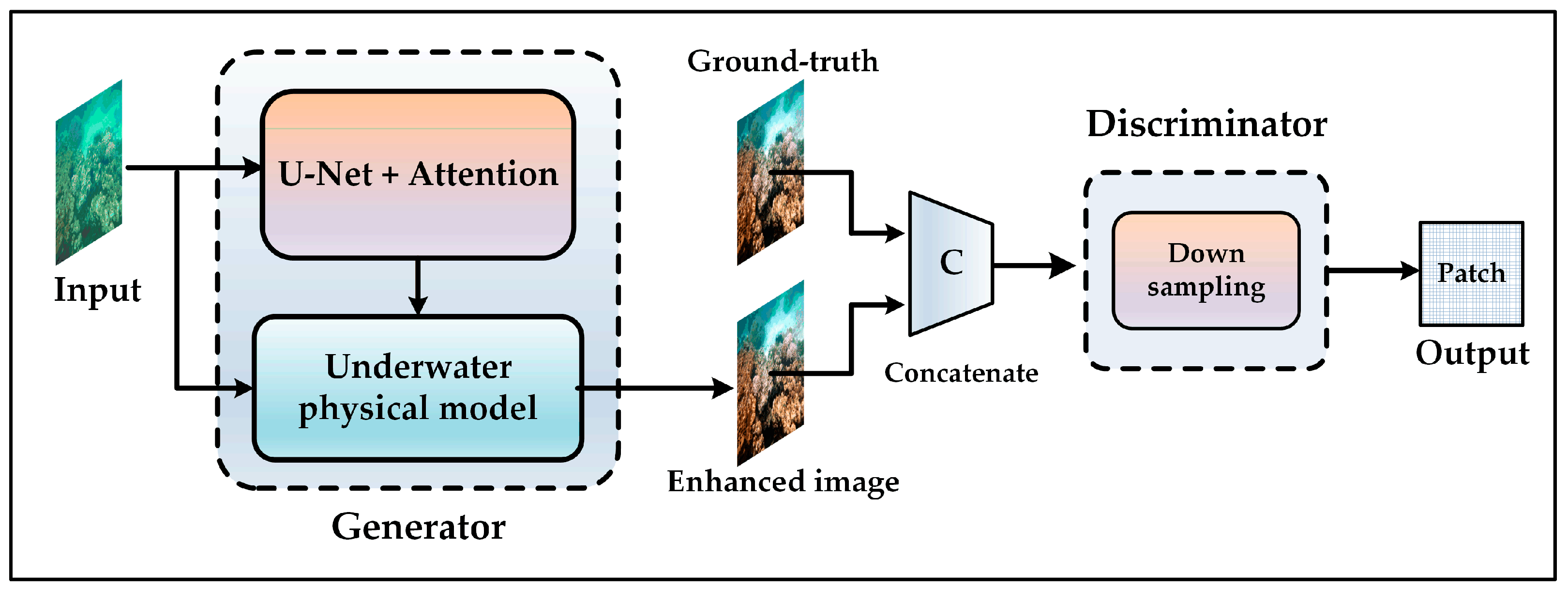
2.1. Generator Network

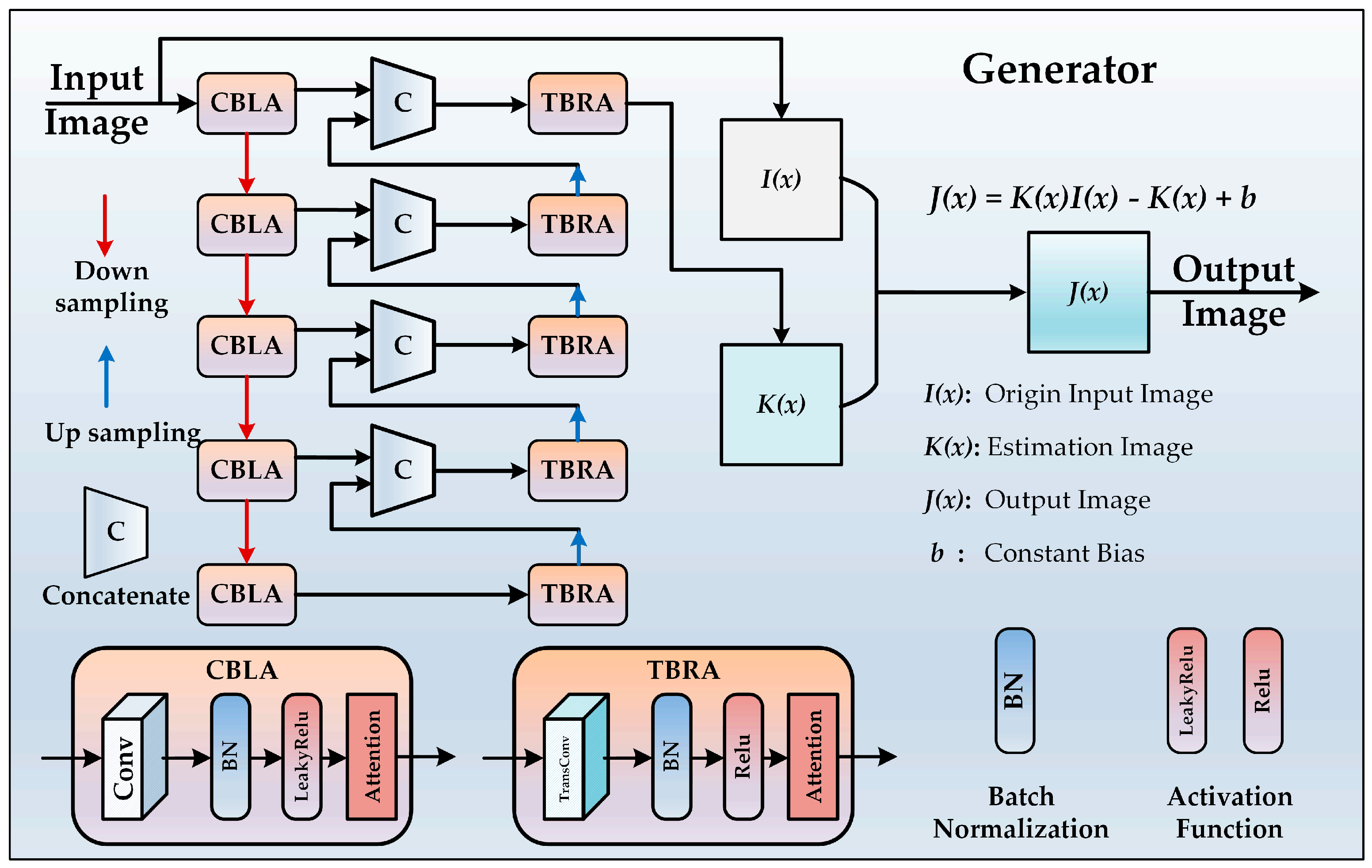
In Figure 2, the structure of the generator is embedded in the down-sampling convolution layer and up-sampling transposed convolution layer of U-Net to form the CBLA module and the TBRA module, respectively, for optimizing the extracted image features. The generator was used to estimate the parameter estimation image of the physical model. Afterward, the real and clear underwater image was inverted by combining the parameter estimation image with the original underwater image.

U-Net is an encoder–decoder network that down-samples the images by using convolution for obtaining low-dimensional features. Then, the network up-samples the features based on transposed convolution to reconstruct the image. In addition, the output of each encoder skip to its corresponding mirror module in decoder preserves the spatial dependence of the encoder. This idea has proved to be effective [31,32].

The structure of U-Net is shown in Figure 3. The input image was reshaped to $256\times 256\times 3$. The low-dimensional feature map of $8\times 8\times 256$ was obtained by using five encoding modules. Afterward, the low-dimensional features and the output of the corresponding decoding module were stacked and used as the input of the decoding module. The encoding module included a 2-D convolution layer with $4\times 4$ kernels and two steps, a batch normalization layer (BN) [33], a leaky ReLU activation function [34], and a channel attention mechanism module. The decoding module included a 2-D transposed convolution layer with $4\times 4$ kernels and two steps, a batch normalization layer, a ReLU activation function [34], and a channel attention mechanism module.

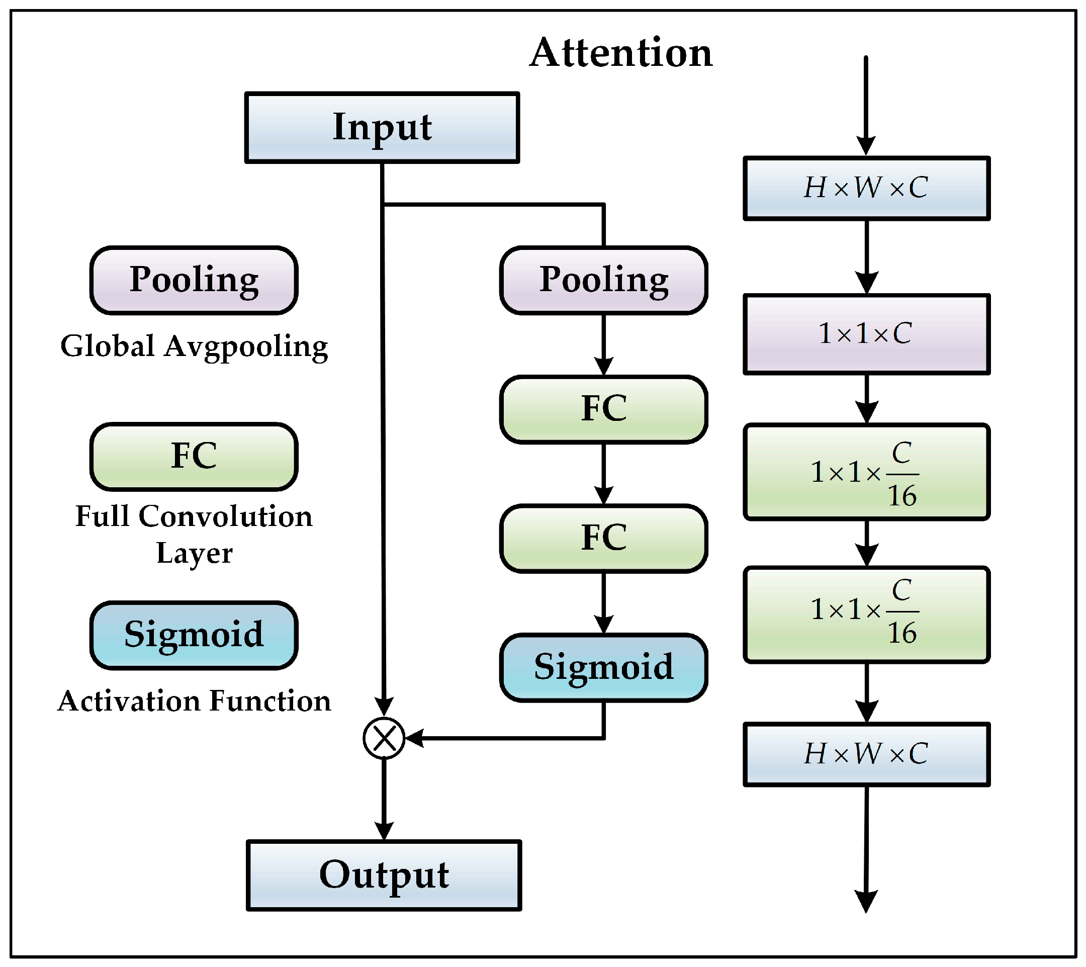
In this model, the channel attention mechanism was added to each convolutional layer and transposed convolutional layer of U-Net as an additional layer of the network to optimize the input features. The specific structure of the module is shown in Figure 4.

The channel attention mechanism first utilized global average pooling to generate channel statistics and then utilized fully connected layers and a sigmoid function to capture channel dependencies [35]. The specific method was to learn the generation of channel weights. The channel attention mechanism could perform feature recalibration and strengthen the feature representation of the network to optimize the parameter estimation of the subsequent physical model.

The first step was the extraction operation, in which an $H\times W\times C$ feature with a height of $H$, a width of $W$, and a channel of $C$ was transformed into $1\times 1\times C$ feature with a global receptive field to a certain extent. The global average pooling is expressed as

$${\mathrm{z}}_c=F_{GAP}\left(x_c\right)=\frac{1}{H\times W}{\displaystyle \sum _{i=1}^H{\displaystyle \sum _{j=1}^W{x}_c\left(i,j\right)}}$$

(1)

where $F_{GAP}\left(x_c\right)$ represents the global average pooling and $x_c\left(i,j\right)$ represents the value of the characteristic of the c-th channel at $\left(i,j\right)$.

Second, the weight generation operation sent the global characteristics of the global average pooling output to two fully connected layers for learning, so as to display the correlation between the geo-modeling channels [16]. Finally, the normalized weight was obtained by the sigmoid function. This is mathematically expressed as

$$s=f\left(W_2\cdot \delta \left(W_1\cdot z_c\right)\right)$$

(2)

where $f$ and $\delta$ represent the sigmoid function and the rectified linear unit (ReLU), respectively. $W_1$ represents the learnable parameters of the first fully connected layer, and $W_2$ represents the learnable parameters of the second layer.

The last step was the scale operation, which weighted the generated weights to the previous features channel by channel and completed the recalibration of the input features on the channels. This is mathematically expressed as follows:

$$\tilde{x}=F_{scale}\left(s\right)\cdot x$$

(3)

where $F_{scale}$ means adjusting the height and width of $s$.

The output of U-Net was used as the input of an underwater physical model [13], which is mathematically expressed as follows:

$$E_T\left(u,v\right)=E_d\left(u,v\right)+E_f\left(u,v\right)+E_b\left(u,v\right)$$

(4)

where $E_T\left(u,v\right),E_d\left(u,v\right),E_f\left(u,v\right),\mathrm{and}{E}_b\left(u,v\right)$ represent the total signal received by the camera, the direct transmission component, the forward scattering component, and the background scattering component, respectively. Since the object was relatively close to the camera, the forward scattering component could be ignored, and only the direct transmission component and the background scattering component were retained [16]. So the underwater optical imaging model was simplified as follows:

$$I\left(x\right)=J(x)t\left(x\right)+B\left(x\right)\left(1-t\left(x\right)\right)$$

(5)

where $I\left(x\right)$ is the observed image, $J\left(x\right)$ is the theoretically real and clear underwater image, and $B\left(x\right)$ represents the background light source. $t\left(x\right)$ is the residual energy ratio after it was captured by the camera, and it is mathematically expressed as follows:

$$t\left(x\right)=e^{-\beta d\left(x\right)}$$

(6)

in which $\beta$ represents the attenuation coefficient of light sources with different wavelengths, and $d\left(x\right)$ represents the distance between the underwater scene and the camera. In order to obtain the real underwater image, $J\left(x\right)$ can be rewritten as follows:

$$J\left(x\right)=\frac{I\left(x\right)+B\left(x\right)t\left(x\right)-B\left(x\right)}{t\left(x\right)}$$

(7)

$t\left(x\right)$ and $B\left(x\right)$ are used as parameters for estimating $K\left(x\right)$ as follows:

$$K\left(x\right)=\frac{\frac{1}{t\left(x\right)}\left(I\left(x\right)-B\left(x\right)\right)+B\left(x\right)}{\left(I\left(x\right)-1\right)}$$

(8)

The final underwater physical model is mathematically expressed as follows:

$$J\left(x\right)=K\left(x\right)I\left(x\right)-K\left(x\right)+b$$

(9)

where $b$ is a constant, which is one by default.

Then, we use the improved U-Net to estimate $K\left(x\right)$, so as to integrate the physical model into the generator. In the architecture of the proposed generator, $I\left(x\right)$ represents the input original underwater image, $K\left(x\right)$ represents the image generated by the generator, $b$ is used as a learnable parameter to fine-tune the final output result, and $J\left(x\right)$ is the final generated image that is sent to the discriminator along with the real sample of the original underwater image.

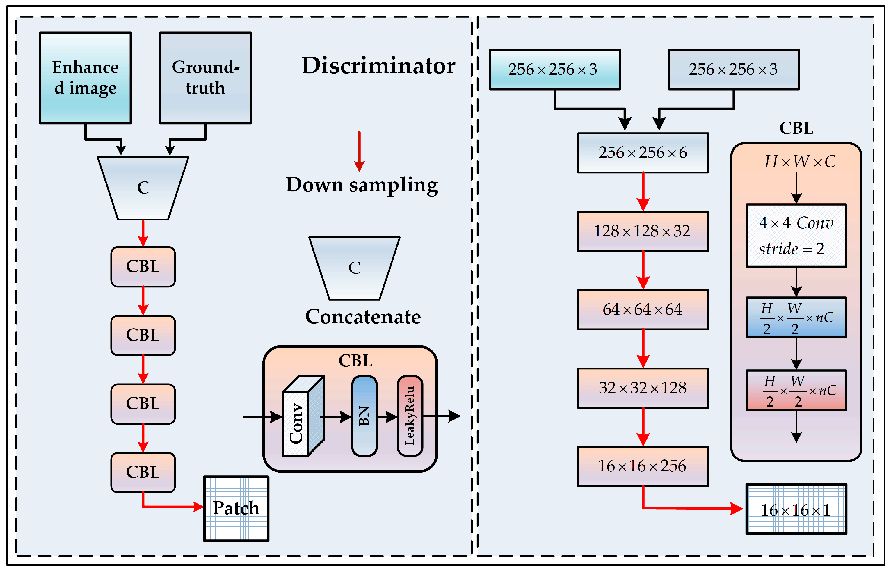
2.2. Discriminator Network

In this work, we used Markovian Patch-GAN [31] as the discriminator. This discriminator is presented in Figure 5. In this structure, we stacked the enhanced image generated by the generator and its corresponding real reference image in the dimension of the channel and then extracted the features by down-sampling the output of the convolution module, which is shown in CBL in Figure 5. The down-sampling module finally outputted a similarity matrix, and the consistency between the images was calculated by the average value of the similarity matrix. This network maintained a fully convolutional structure to a certain extent and at the same time achieved the function of judging images.

The main operation of the discriminator was to transform two enhanced images of $256\times 256\times 3$ and real reference images into images of size $256\times 256\times 6$ by stacking and then reduce the dimensions by using the down-sampling module for four consecutive times. Each down-sampling module reduced the width and height of the images to half of the original image and outputted them as a similar matrix of $16\times 16$. Finally, the module averaged the values of the matrix. The down-sampling module contained a two-dimensional convolution layer with a kernel of $4\times 4$ and a step size of 2, a batch normalization layer (BN), and a leaky-ReLU activation function.

2.3. Loss Function

The loss function was mainly used to guide the network model parameters in the direction of minimum loss. In this paper, we designed a loss function that integrated the adversarial loss, the global loss, and the perceptual loss to guide the training of the generative adversarial network.

The adversarial loss was caused by the game between the generator and discriminator. The generator constantly updated the network parameters to generate an image consistent with the real reference image. On the other hand, the discriminator continuously judged whether the generated image was original or fake.

$$\underset{G}{\min }\underset{D}{\max }{L}_{GAN}\left(G,D\right)={\mathbb{E}}_{X,Y}\left[\log D\left(Y\right)\right]+{\mathbb{E}}_{X,Y}\left[\log \left(1-D\left(X,G\left(X\right)\right)\right)\right]$$

(10)

where $G$ represents the generator, $D$ represents the discriminator, $X$ represents the source domain (low-quality underwater image), and $Y$ represents the target domain (clear underwater image). The generator $G$ aims to minimize the loss $L_{GAN}$, while the discriminator aims to maximize $L_{GAN}$.

Many current methods show that adding $L_1$ or $L_2$ loss can result in the images generated by the generator having a better global similarity [31,36]. It is noteworthy that the $L_2$ loss is less robust, and it is easier to introduce blur in the image. In this paper, the $L_1$ loss (global loss) had a better effect and is expressed as follows:

$$L_1\left(G\right)={\mathbb{E}}_{X,Y}\left[{\Vert Y-G\left(X\right)\Vert }_1\right]$$

(11)

The perceptual loss was beneficial for making the generator $G$ attain the texture information of the image. According to its calculation method, we defined the perceptual loss $\Phi ()$. In this method, the features in the generated image and the real image were extracted by using VGG-19. The Euclidean distance between the high-dimensional feature maps extracted by them in block5_conv2 layer was calculated. The VGG-19 is a pre-trained network. The perceptual loss is mathematically expressed as follows:

$$L_{content}={\mathbb{E}}_{X,Y}\left[{\Vert \Phi \left(Y\right)-\Phi \left(G\left(X\right)\right)\Vert }_2\right]$$

(12)

The adversarial loss, the global loss, and the perceptual loss were combined, and the following loss function was obtained:

$$G^{*}=\arg \underset{G}{\min }\underset{D}{\max }{L}_{GAN}\left(G,D\right)+{\lambda }_1{L}_1\left(G\right)+{\lambda }_2{L}_{content}\left(G\right)$$

(13)

where ${\lambda }_1$ and ${\lambda }_2$ are hyperparameters, which are used to adjust the proportion of global loss and perceptual loss in the loss function. In order to select the appropriate hyperparameters so that the fusion loss could achieve the optimal effect, we referred to the previous work [25] and determined the value range of the two hyperparameters to be (0, 1). Then, under the same experimental conditions, we fine-tuned the parameters with a step size of 0.1 and recorded the loss on the EUVP dataset, and the final results are shown in Figure 6. The experiments showed that ${\lambda }_1=0.7,{\lambda }_2=0.3$ had the best effect.

2.4. Image Evaluation Metrics

For evaluating the image quality, this study adopted well-known image evaluation metrics, such as peak signal-to-noise ratio (PSNR) [17,32] and structural similarity (SSIM) [37]. The commonly used evaluation metrics in underwater image processing include underwater image quality measure (UIQM) [38] and underwater color image quality evaluation (UCIQE) [39].

The PSNR was obtained by calculating the mean square error (MSE) between the generated image and the real value of the original input. This is mathematically expressed as follows:

$$PSNR\left(x,y\right)=10{\log }_{10}\left[\frac{{255}^2}{MSE\left(x,y\right)}\right]$$

(14)

where $x$ and $y$ represent the real values of the generated image and the original image, respectively. The $MSE\left(x,y\right)$ represents the mean square error between the generated image and the original image. The larger the value of PSNR, the lower was the noise in the image.

The natural image had strong correlations between each channel and each pixel value in the channel. These correlations contained important feature information regarding the object structure in the visual scene. The SSIM refers to the difference in brightness, contrast, and structure between two images. The SSIM was computed by using the expression

$$SSIM\left(x,y\right)=\left(\frac{2{\mu }_x{\mu }_y+c_1}{{\mu }_x^2+{\mu }_y^2+c_1}\right)\left(\frac{2{\sigma }_{xy}+c_2}{{\sigma }_x^2+{\sigma }_y^2+c_2}\right)$$

(15)

where $x$ and $y$ represent the real values of the generated image and the original image, respectively; ${\mu }_x({\mu }_y)$ represents the average value of each channel of the image; ${\sigma }_x({\sigma }_y)$ represents the variance of each channel of the image; and ${\sigma }_{xy}$ represents the covariance between $x$ and $y$. In addition, $c_1$ and $c_2$ were used to ensure the stability of the numerical values. The larger the value of SSIM, the more similar were the structures of the two images.

The UIQM is a special metric for evaluating the underwater image quality proposed by Panetta et al. [40]. This metric did not need the real value corresponding to the original image. The UIQM obtained the final result by quantifying the color, sharpness, and contrast and weighting it. This is expressed as

$$UIQM\left(x\right)=w_{1}UICM\left(x\right)+w_{2}UISM\left(x\right)+w_{3}UIConM\left(x\right)$$

(16)

where $x$ represents the test image. $UICM\left(x\right)$, $UISM\left(x\right)$, and $UIConM\left(x\right)$ represent the color, definition, and contrast of the quantized image, respectively, and $w_1$, $w_2$, and $w_3$ represent the weight of each component. As the value of metric became larger, the color of the image was closer to the image in the normal state.

UCIQE is a new measurement method proposed by Yang et al. [39]. The method compared the pixels per inch distribution of underwater images in CIELAB color space with subjective image quality perception. This method was a linear combination of chromaticity, saturation, and contrast, and was used to quantify the uneven color projection, blur, and low contrast of the underwater images. The metric is mathematically expressed as follows:

$$UCIQE\left(x\right)=c_1\times {\sigma }_c+c_2\times co{n}_l+c_3\times {\mu }_s$$

(17)

where $x$ is the test image; ${\sigma }_c$ is the standard deviation of chromaticity; $co{n}_l$ is the brightness contrast; μ_s is the average value of saturation; and $c_1$, $c_2$, and $c_3$ are the weighting coefficients. The larger the value of this metric was, the thicker was the color of the image.

3. Results and Discussion

In order to verify the effectiveness of the proposed method, we trained and tested it by using two publicly available datasets, including the enhancement of the underwater visual perception (EUVP) [25] dataset and the underwater image enhancement benchmark dataset (UIEBD) [41]. Then, we compared the proposed method with model-based methods, such as the depth estimation method of an underwater scene based on image blur and light absorption (IBLA) [42], the depth of field estimation model of an underwater image based on underwater light attenuation prior (ULAP) [43], and CBM [44]; CNN-based methods, including WaterNet [41] and an enhanced model based on structural decomposition and underwater imaging characteristics (UWCNN) [45]; and GAN-based methods, including multilevel feature fusion-based conditional GAN (MLFcGAN) [46], UGAN [6], fast underwater image enhancement for improved visual perception (FunieGAN) [25], based on a physical model and a GAN network (IPMGAN) [20], and a comprehensive underwater object tracking benchmark dataset and underwater image enhancement with GAN (CRN-UIE) [47] in terms of visual quality, quantitative criteria, and real-time performance.

3.1. Dataset Introduction

EUVP was a large dataset, which comprised 13,000 pairs of underwater images for training and verification and 515 pairs of test images for testing the generalization ability of the model. Seven different cameras were used in the EUVP dataset to obtain underwater images. In addition, the dataset also included images extracted from some public videos to adapt to a wide range of underwater scenes. This dataset mainly contained underwater scenes with blue, green, and low brightness. Based on this dataset, we could test the ability of color correction and brightness enhancement of the model.

The UIEBD contained 950 large-resolution underwater images. These image data came from Google and some related papers, and after refinement, they contained different underwater scenes, mainly statues and marine life. The corresponding reference images were generated by using 12 different image enhancement algorithms and were selected by pairwise comparison. Finally, 890 pairs of underwater images and 60 underwater images without reference were obtained. This dataset mainly included blue, green, and fuzzy underwater scenes, which could be used for testing the ability of the color correction and clarity improvement of the model.

3.2. Experimental Setup

The proposed method was implemented by using PyTorch (1.2.0). We used TD41-Z2 server manufactured by AMAX (Suzhou, China), with internal configurations including CPU Intel (R) Xeon (R) Silver4210R CPU @ 2.40 GHz, NVIDIA 3090 GPU, and 256 GB RAM. The network was trained for 400 epochs on the EUVP and UIEBD datasets. During the training process, we used the batch size of 64, an Adam optimizer, an initial learning rate of 0.001, and an exponential attenuation rate, and the input image size was adjusted to $256\times 256$.

3.3. Evaluation of Visual Quality

First, we evaluated the image quality from the visual aspect. We randomly selected five images from the training sets of the two aforementioned datasets and analyzed them by comparing the original input image, the real reference image, and the enhanced image. Some example images are shown in Figure 7.

From the EUVP dataset, the real color of the enhanced image was restored, the color deviation of blue and green was solved, and the brightness was improved to a certain extent. However, the color concentration was not as good as that of the real reference image. In the UIEBD dataset, in addition to the correction of the color deviation, it had a certain effect on image defogging, but it lacked improvements in color saturation, and the enhancement effect of some bright areas in the image required improvement.

The proposed method was compared with 10 advanced underwater image enhancement algorithms. For the models that required training, such as WaterNet [41], CRN-UIE [47], etc., we trained and verified them based on the training sets of EUVP and UIEBD according to the network structure and training parameter settings described in this work and randomly selected five images from the two test sets for performing the analysis. The corresponding results are shown in Figure 8 and Figure 9.

As shown in Figure 8, in the EUVP dataset, the original image had some problems, such as the green color, the blue color, and low brightness. The IBLA and ULAP methods based on the physical model improved the brightness, but the color deviation was not corrected completely. The images generated by MLFcGAN, UGAN, and FunieGAN based on GAN had higher contrast. However, the images were still green. The image enhanced by CBM was different from the reference image, but the visual performance was better, which may have been due to the fact that CBM was based on morphological operations without a reference image. The brightness of the UWCNN-enhanced image was obviously improved, but there was a phenomenon of supersaturation. The image generated by CRN-UIE was closer to the reference image. The proposed method and WaterNet had better performance in color deviation correction, the proposed method was better in brightness improvement, and there was room for further improvement in color density.

As shown in Figure 9, based on the UIEBD dataset, the color supersaturation problem of the IBLA and ULAP methods may have been due to the serious degradation of the dataset. This led to inaccurate prior parameter estimation, when these methods generated transmission images. The CBM method used the morphological processing for restraining the problem of supersaturation. The WaterNet and MLFcGAN had some correction effects on color deviation, but they were not good enough in terms of defogging. There was a certain difference between the images generated by UWCNN and the reference image, which may have been due to insufficient training epochs. UGAN and IPMGAN were superior to other methods in image defogging. Our method was similar to CRN-UIE in color correction but had certain advantages in contrast enhancement. The method may have had the problem of background color deviation when enhancing low-brightness images, and the defogging effect was not particularly ideal.

3.4. Quantization Comparison of Enhanced Images

To verify the generalization performance of different methods based on EUVP datasets, the advanced underwater image enhancement methods were learned by using the training set and tested by the standard test set provided by EUVP. The corresponding results are shown in

Table 1. Underwater image quality evaluation of different enhancement methods on EUVP.

Method	PSNR (dB) ↑	SSIM ↑	UIQM ↑	UCIQE ↑
Original image	(17.27, 2.88)	(0.62, 0.07)	(2.67, 0.52)	(0.57, 0.05)
Reference image	-	-	(2.88, 0.54)	(0.59, 0.05)
IBLA [42]	(22.11, 4.72)	(0.73, 0.14)	(2.16, 0.56)	(0.62, 0.05)
ULAP [43]	(21.92, 2.54)	(0.72, 0.09)	(2.17, 0.56)	(0.61, 0.04)
CBM [44]	(21.22, 2.96)	(0.72, 0.07)	(2.78, 0.41)	(0.63, 0.03)
WaterNet [41]	(24.06, 3.71)	(0.78, 0.07)	(3.07, 0.38)	(0.60, 0.03)
UWCNN [45]	(20.02, 3.42)	(0.71, 0.09)	(3.02, 0.24)	(0.63, 0.05)
MLFcGAN [46]	(25.52, 2.53)	(0.76, 0.07)	(2.91, 0.46)	(0.59, 0.04)
UGAN [6]	(26.55, 3.16)	(0.81, 0.05)	(2.96, 0.43)	(0.59, 0.05)
FunieGAN [25]	(25.46, 3.03)	(0.77, 0.06)	(2.96, 0.41)	(0.59, 0.04)
IPMGAN [20]	(23.54, 3.11)	(0.78, 0.07)	(3.08, 0.36)	(0.58, 0.03)
CRN-UIE [47]	(25.58, 2.98)	(0.79, 0.06)	(3.11, 0.26)	(0.61, 0.03)
Ours	(26.93, 3.22)	(0.79, 0.06)	(3.13, 0.38)	(0.59, 0.03)

, where red indicates the best result, and blue indicates the suboptimal result. The former indicates the mean, and the latter indicates the variance in brackets. The symbol “↑” means that the larger the metric, the higher the image quality.

According to the comparison results based on PSNR and SSIM, which paid attention to image similarity, our method achieved the optimal and suboptimal results, respectively. On one hand, the channel attention mechanism improved the utilization performance of the features. On the other hand, the fusion loss function enhanced the texture details and suppressed noise. The processing results of UGAN were also outstanding as the mapping relationship was excellent, which caused the generated image to be closest to the reference image. In terms of unreferenced UIQM and UCIQE, the method proposed in this paper had a remarkable effect on UIQM considering underwater characteristics because of the underwater physical model. In terms of UCIQE, the proposed method had no advantage because the color of some areas in the enhanced image was weak.

In order to verify the generalization performance of different methods on UIEBD, we used 60 unreferenced underwater images provided by UIEBD. As these 60 images were more degraded as compared with the 890 trained images, there were no clear and referenceable images for the time being. Therefore, only UIQM and UCIQE metrics were used for performing comparison. The results are shown in

Table 2. Underwater image quality evaluation of different enhancement methods on UIEBD.

Method	UIQM ↑	UCIQE ↑
Original image	(2.163, 0.631)	(0.517, 0.064)
IBLA [42]	(2.132, 0.567)	(0.584, 0.064)
ULAP [43]	(1.807, 0.702)	(0.565, 0.068)
CBM [44]	(2.718, 0.508)	(0.635, 0.031)
WaterNet [41]	(2.887, 0.374)	(0.570, 0.033)
UWCNN [45]	(2.789, 0.732)	(0.623, 0.039)
MLFcGAN [46]	(2.622. 0.473)	(0.589, 0.052)
UGAN [6]	(2.574, 0.571)	(0.568, 0.044)
FunieGAN [25]	(2.775, 0.512)	(0.573, 0.057)
IPMGAN [20]	(2.782, 0.611)	(0.574, 0.062)
CRN-UIE [47]	(2.788, 0.713)	(0.591, 0.044)
Ours	(2.789, 0.622)	(0.579, 0.043)

, where red indicates the best result, and blue indicates the suboptimal result. The former indicates the mean, and the latter indicates the variance in brackets. The symbol “↑” means that the larger the metric, the higher the image quality.

The comparison results show that WaterNet performed best on UIQM, which may have been due to the fact that it used different image enhancement methods to fuse images, so that the best results could be achieved by learning the color, brightness, and contrast of the images through CNNs. However, the proposed method had better robustness when facing different underwater scenes due to the existence of underwater physical models, so it achieved suboptimal results. Based on UCIQE, the image color was heavy because of supersaturation, so the value of IBLA was high, but the visual quality was defective. On the other hand, because of the morphological processing of CBM, the visual performance was good, and the evaluation metric also reached the best result. However, the color of the image generated by the proposed method was light, so there was a slight gap in UCIQE as compared with the method based on the physical model.

To evaluate the performance of the model, we performed five-fold cross-validation on EUVP and UIEBD datasets. We randomly divided all the data into five parts, one of which was used as the test set and the rest as the training set, and exchanged them in sequence. The specific results of the mean and standard deviation (SD) in five experiments are shown in

Table 3. Five-fold cross-validation on EUVP dataset.

Fold	PSNR (dB)	SSIM	UIQM	UCIQE
1	26.88	0.77	3.15	0.57
2	25.74	0.81	3.11	0.58
3	26.99	0.79	3.09	0.57
4	26.79	0.79	3.14	0.59
5	27.01	0.78	3.12	0.59
Average	26.68	0.79	3.12	0.58
SD	0.53	0.02	0.02	0.01

and

Table 4. Five-fold cross-validation on UIEBD dataset.

Fold	PSNR (dB)	SSIM	UIQM	UCIQE
1	23.21	0.68	2.67	0.56
2	25.86	0.62	2.78	0.58
3	26.01	0.71	2.73	0.55
4	23.17	0.74	2.59	0.57
5	24.58	0.69	2.77	0.57
Average	24.56	0.68	2.71	0.57
SD	1.37	0.04	0.08	0.01

.

Since the images in the same dataset did not have significant differences with each other, our model results were relatively stable via random partitioning.

Finally, we compared the various algorithms in Table 1 using the Iman–Davenport test method in the scmamp package proposed by Calvo et al. [48], and the p-values are shown in

Table 5. Different test methods using p-value statistics on two datasets.

	Without Our Method	With Our Method
EUVP	4.08 × 10−1	3.26 × 10−1
UIEBD	1.49 × 10−1	2.15 × 10−1

. Compared with other methods, our model did not generate significant results.

3.5. Ablation Experiments

Then, four evaluation metrics, including PSNR, SSIM, UIQM, and UCIQE, were used to perform ablation experiments. The standard test set provided by EUVP was used, and the corresponding results are shown in

Table 6. Underwater image quality evaluation of different variants of the proposed method.

CA	UPM	FL	PSNR (dB) ↑	SSIM ↑	UIQM ↑	UCIQE ↑
			(25.46, 3.03)	(0.76, 0.06)	(2.88, 0.47)	(0.57, 0.04)
√			(26.94, 3.09)	(0.80, 0.07)	(2.97, 0.44)	(0.58, 0.05)
√	√		(24.90, 3.41)	(0.79, 0.08)	(3.09, 0.38)	(0.59, 0.03)
√	√	√	(26.92, 3.22)	(0.79, 0.06)	(3.13, 0.38)	(0.59, 0.03)

, where red denotes the best result, and blue denotes the second-best result. The former indicates the mean, and the latter indicates the variance in brackets.

After adding the channel attention mechanism in the generator, the four indexes increased by 5.96%, 44.31%, 3.22%, and 1.7%. The channel attention (CA) mechanism improved the utilization performance of the features and caused the image generated by the model to be closer to the reference image. As a result, it achieved the best results in terms of PSNR and SSIM. The simplified underwater physical model (UPM) enhanced the image from the underwater imaging characteristics and did not completely depend on the reference image. Therefore, the UIQM and UCIQE increased by 7.35% and 1.7% after incorporating UPM in the generator, but the PSNR and SSIM were reduced. The global loss and perceptual loss effectively restored the texture information of the image and suppressed noise, so that the PSNR and UIQM were improved by integrating the global loss and perceptual loss into the fusion loss (FL). However, the color density in the image generated by the method was too weak. Therefore, the improvement in UCIQE was not obvious.

The PSNR and SSIM metrics mainly focused on the similarity between the enhanced image and the reference image. The closer enhanced image was to the reference image, the higher was the score. The model improved the ability to extract effective features after adding the channel attention mechanism and enhanced the feature representation ability of U-Net, thus reducing the difference between the generated image and the reference image. As shown in Table 6, our method achieved good results in PSNR and SSIM.

It is worth noting that the reference images did not always have the best visual effect. In Table 1, the UIQM and UCIQE values of the real images were slightly lower as compared with those of the images generated by using deep learning methods, which actually limited the performance of the models. We embedded the underwater physical model in the generator, so that the generator was able to enhance the images in terms of underwater imaging characteristics. This reduced the dependence on the reference images to some extent, thus improving the UIQM and PSNR metrics for underwater image evaluation. However, at the same time, it reduced the PSNR and SSIM metrics based on the reference image.

In terms of loss function, we combined the adversarial loss, the global loss, and the perceptual loss. The latter two effectively restored the texture details of an image and suppressed the noise in the image, so that it could improve the PSNR that paid attention to the proportion of information. In addition, our method corrected the color deviation, improved the brightness, and appeared clearer. Therefore, it performed well on UIQM, as shown in Table 1. However, there was a lack of color saturation, and the enhancement effect on UCIQE metric was not obvious. In addition, we observed that when the color of the enhanced image was too bright, the UCIQE was high. Therefore, if the image was supersaturated, UCIQE was inconsistent with the actual visual experience.

3.6. Real-Time Analysis and Discussion

We used the published underwater target tracking dataset UOT32 [49] to compare the practicability of the advanced underwater image enhancement methods. We used the video sequences naturally shot in it and adjusted the resolution of each frame to adapt to the input of the model. With regard to different image enhancement methods, we counted the parameters of different network models and analyzed the relationship between the parameters and the image processing speed. Then, we conducted experiments on TD41-Z2 server made by AMAX (Suzhou, China) with GPU (NVIDIA RTX 3090), and averaged the processing results, as shown in

Table 7. Underwater image processing speed of different enhancement methods on UOT32.

Method	Size	FPS
IBLA [42]	-	1.8
ULAP [43]	-	2.5
CBM [44]	-	45.3
WaterNet [41]	157.3 M	105.8
UWCNN [45]	1.1 M	32.3
MLFcGAN [46]	565.6 M	84.9
UGAN [6]	654.2 M	73.6
FunieGAN [25]	21.9 M	138.5
IPMGAN [20]	323.5 M	91.4
CRN-UIE [47]	59.6 M	112.3
Ours	27.1 M	121.7

, where red indicates the best result, and blue indicates the suboptimal result.

As the physical model-based methods IBLA and ULAP adjusted every pixel, the processing time was longer as compared with the learning-based method, which could not meet the real-time requirements. As compared with general methods, CRN-UIE was a target-oriented tracking method, so its real-time performance was better. Although UWCNN had the smallest network scale, its real-time performance was not outstanding, because it needed physical models to generate additional transmission images. The network scale of FunIEGAN and our method was smaller as compared with other methods, and the processing speed was optimal and suboptimal, respectively. Therefore, this method is competitive in actual underwater work.

4. Conclusions

In this paper, a network model for underwater image enhancement was proposed. In this model, the channel attention mechanism was embedded in U-Net, which suppressed the noise existing in the original image and restored the real color of the image by combining with the underwater physical model. In addition, the existence of the underwater physical model also alleviated the problem that the generator was highly dependent on specific datasets. In order to verify the effectiveness of the proposed method, we trained and tested it on EUVP and UIEBD and compared the results with some advanced underwater image enhancement algorithms. The results showed that in the visual effect, the color deviation of the enhanced image was corrected, and the high-noise problem was solved. In the image evaluation metrics, our method performed well on PSNR and UIQM, indicating that the noise of the image was suppressed, and the color was balanced. In practical applications, the proposed method was competitive in real-time processing speed. This method improved the brightness to a certain extent, but some areas in the enhanced image were lighter in color, which was manifested by a lower UCIQE. In addition, we did not consider the influence of underwater depth, light level, and water turbulence on the original image, so it had certain limitations. In the future, we will continue to optimize the proposed structure for enhancing the saturation of color and pay attention to the acquisition methods of underwater images and significance testing of the model.

References

1. Raveendran, S.; Patil, M.D.; Birajdar, G.K. Underwater image enhancement: A comprehensive review, recent trends, challenges and applications. Artif. Intell. Rev. 2021, 54, 5413–5467. [Google Scholar] [CrossRef]
2. Zhang, W.; Zhuang, P.; Sun, H.H.; Li, G.; Kwong, S.; Li, C. Underwater Image Enhancement via Minimal Color Loss and Locally Adaptive Contrast Enhancement. IEEE Trans. Image Process. 2022, 31, 3997–4010. [Google Scholar] [CrossRef] [PubMed]
3. Paull, L.; Seto, M.; Leonard, J.J.; Li, H. Probabilistic cooperative mobile robot area coverage and its application to autonomous seabed mapping. Int. J. Robot. Res. 2018, 37, 21–45. [Google Scholar] [CrossRef]
4. Akkaynak, D.; Treibitz, T.; Shlesinger, T.; Loya, Y.; Tamir, R.; Iluz, D. What is the Space of Attenuation Coefficients in Underwater Computer Vision? In Proceedings of the 2017 IEEE Conference on Computer Vision and Pattern Recognition (CVPR), Honolulu, HI, USA, 21–26 July 2017; pp. 568–577. [Google Scholar]
5. Akkaynak, D.; Treibitz, T. A Revised Underwater Image Formation Model. In Proceedings of the 2018 IEEE/CVF Conference on Computer Vision and Pattern Recognition (CVPR), Salt Lake City, UT, USA, 18–23 June 2018; pp. 6723–6732. [Google Scholar]
6. Fabbri, C.; Islam, M.J.; Sattar, J. Enhancing underwater imagery using generative adversarial networks. In Proceedings of the 2018 IEEE International Conference on Robotics and Automation (ICRA), Brisbane, Australia, 21–25 May 2018; pp. 7159–7165. [Google Scholar]
7. Cazau, D.; Bonnel, J.; Baumgartner, M. Wind Speed Estimation Using Acoustic Underwater Glider in a Near-Shore Marine Environment. IEEE Trans. Geosci. Remote Sens. 2019, 57, 2097–2106. [Google Scholar] [CrossRef]
8. Bloisi, D.D.; Previtali, F.; Pennisi, A.; Nardi, D.; Fiorini, M. Enhancing Automatic Maritime Surveillance Systems with Visual Information. IEEE Trans. Intell. Transp. Syst. 2017, 18, 824–833. [Google Scholar] [CrossRef] [Green Version]
9. Sheinin, M.; Schechner, Y.Y. The Next Best Underwater View. In Proceedings of the 2016 IEEE Conference on Computer Vision and Pattern Recognition (CVPR), Las Vegas, NV, USA, 27–30 June 2016; pp. 3764–3773. [Google Scholar]
10. Pizer, S.M.; Amburn, E.P.; Austin, J.D.; Cromartie, R.; Geselowitz, A.; Greer, T.; ter Haar Romeny, B.; Zimmerman, J.B.; Zuiderveld, K. Adaptive histogram equalization and its variations. Comput. Vis. Graph. Image Process. 1987, 39, 355–368. [Google Scholar] [CrossRef]
11. Ching-Chih, W.; Chen, H.; Chiou-Shann, F. A novel automatic white balance method for digital still cameras. In Proceedings of the 2005 IEEE International Symposium on Circuits and Systems (ISCAS), Kobe, Japan, 23–26 May 2005; Volume 4, pp. 3801–3804. [Google Scholar]
12. Han, M.; Lyu, Z.; Qiu, T.; Xu, M. A review on intelligence dehazing and color restoration for underwater images. IEEE Trans. Syst. Man Cybern. Syst. 2018, 50, 1820–1832. [Google Scholar] [CrossRef]
13. Jaffe, J.S. Computer modeling and the design of optimal underwater imaging systems. IEEE J. Ocean. Eng. 1990, 15, 101–111. [Google Scholar] [CrossRef]
14. He, K.; Sun, J.; Tang, X. Single Image Haze Removal Using Dark Channel Prior. IEEE Trans. Pattern Anal. Mach. Intell. 2011, 33, 2341–2353. [Google Scholar]
15. Yang, H.; Chen, P.; Huang, C.; Zhuang, Y.; Shiau, Y. Low Complexity Underwater Image Enhancement Based on Dark Channel Prior. In Proceedings of the 2011 Second International Conference on Innovations in Bio-Inspired Computing and Applications, Shenzhen, China, 16–18 December 2011; pp. 17–20. [Google Scholar]
16. Li, H.; Zhang, C.; Wan, N.; Chen, Q.; Wang, D.; Song, D. An Improved Method for Underwater Image Super-Resolution and Enhancement. In Proceedings of the 2021 IEEE 4th International Conference on Electronics Technology (ICET), Chengdu, China, 7–10 May 2021; pp. 1295–1299. [Google Scholar]
17. Ignatov, A.; Kobyshev, N.; Timofte, R.; Vanhoey, K.; Van Gool, L. Dslr-quality photos on mobile devices with deep convolutional networks. In Proceedings of the IEEE International Conference on Computer Vision (ICCV), Venice, Italy, 22–29 October 2017; pp. 3277–3285. [Google Scholar]
18. Wang, Y.; Zhang, J.; Cao, Y.; Wang, Z. A deep CNN method for underwater image enhancement. In Proceedings of the 2017 IEEE International Conference on Image Processing (ICIP), Beijing, China, 17–20 September 2017; pp. 1382–1386. [Google Scholar]
19. Barbosa, W.V.; Amaral, H.G.B.; Rocha, T.L.; Nascimento, E.R. Visual-Quality-Driven Learning for Underwater Vision Enhancement. In Proceedings of the 2018 25th IEEE International Conference on Image Processing (ICIP), Athens, Greece, 7–10 October 2018; pp. 3933–3937. [Google Scholar]
20. Liu, X.; Gao, Z.; Chen, B.M. IPMGAN: Integrating physical model and generative adversarial network for underwater image enhancement. Neurocomputing 2021, 453, 538–551. [Google Scholar] [CrossRef]
21. Goodfellow, I.; Pouget-Abadie, J.; Mirza, M.; Xu, B.; Warde-Farley, D.; Ozair, S.; Courville, A.; Bengio, Y. Generative adversarial nets. Adv. Neural Inf. Process. Syst. 2014, 27, 5413–5467. [Google Scholar]
22. Li, J.; Skinner, K.A.; Eustice, R.M.; Johnson-Roberson, M. WaterGAN: Unsupervised Generative Network to Enable Real-Time Color Correction of Monocular Underwater Images. IEEE Robot. Autom. Lett. 2018, 3, 387–394. [Google Scholar] [CrossRef] [Green Version]
23. Zhu, J.; Park, T.; Isola, P.; Efros, A.A. Unpaired Image-to-Image Translation Using Cycle-Consistent Adversarial Networks. In Proceedings of the 2017 IEEE International Conference on Computer Vision (ICCV), Venice, Italy, 22–29 October 2017; pp. 2242–2251. [Google Scholar]
24. Mirza, M.; Osindero, S. Conditional generative adversarial nets. arXiv 2014, arXiv:1411.1784. [Google Scholar]
25. Islam, M.J.; Xia, Y.; Sattar, J. Fast underwater image enhancement for improved visual perception. IEEE Robot. Autom. Lett. 2020, 5, 3227–3234. [Google Scholar] [CrossRef] [Green Version]
26. Hambarde, P.; Murala, S.; Dhall, A. UW-GAN: Single-image depth estimation and image enhancement for underwater images. IEEE Trans. Instrum. Meas. 2021, 70, 5018412. [Google Scholar] [CrossRef]
27. Gu, J.; Hu, H.; Wang, L.; Wei, Y.; Dai, J. Learning region features for object detection. In Proceedings of the European Conference on Computer Vision (ECCV), Munich, Germany, 8–14 September 2018; pp. 381–395. [Google Scholar]
28. Hu, H.; Gu, J.; Zhang, Z.; Dai, J.; Wei, Y. Relation networks for object detection. In Proceedings of the IEEE conference on Computer Vision and Pattern Recognition (CVPR), Salt Lake City, UT, USA, 18–23 June 2018; pp. 3588–3597. [Google Scholar]
29. Zhao, H.; Zhang, Y.; Liu, S.; Shi, J.; Loy, C.C.; Lin, D.; Jia, J. Psanet: Point-wise spatial attention network for scene parsing. In Proceedings of the European Conference on Computer Vision (ECCV), Munich, Germany, 8–14 September 2018; pp. 267–283. [Google Scholar]
30. Ronneberger, O.; Fischer, P.; Brox, T. U-Net: Convolutional Networks for Biomedical Image Segmentation. In Proceedings of the Medical Image Computing and Computer-Assisted Intervention—MICCAI 2015, Munich, Germany, 5–9 October 2015; pp. 234–241. [Google Scholar]
31. Isola, P.; Zhu, J.; Zhou, T.; Efros, A.A. Image-to-Image Translation with Conditional Adversarial Networks. In Proceedings of the 2017 IEEE Conference on Computer Vision and Pattern Recognition (CVPR), Honolulu, HI, USA, 21–26 July 2017; pp. 5967–5976. [Google Scholar]
32. Chen, Y.; Wang, Y.; Kao, M.; Chuang, Y. Deep Photo Enhancer: Unpaired Learning for Image Enhancement from Photographs with GANs. In Proceedings of the 2018 IEEE/CVF Conference on Computer Vision and Pattern Recognition (CVPR), Salt Lake City, UT, USA, 18–23 June 2018; pp. 6306–6314. [Google Scholar]
33. Ioffe, S.; Szegedy, C. Batch normalization: Accelerating deep network training by reducing internal covariate shift. In Proceedings of the International Conference on Machine Learning (ICML), Lille, France, 6–11 July 2015; pp. 448–456. [Google Scholar]
34. Maas, A.L.; Hannun, A.Y.; Ng, A.Y. Rectifier nonlinearities improve neural network acoustic models. In Proceedings of the International Conference on Machine Learning (ICML), Atlanta, GA, USA, 16–21 June 2013; p. 3. [Google Scholar]
35. Hu, J.; Shen, L.; Sun, G. Squeeze-and-Excitation Networks. In Proceedings of the 2018 IEEE/CVF Conference on Computer Vision and Pattern Recognition (CVPR), Salt Lake City, UT, USA, 18–23 June 2018; pp. 7132–7141. [Google Scholar]
36. Yu, X.; Qu, Y.; Hong, M. Underwater-GAN: Underwater image restoration via conditional generative adversarial network. In Proceedings of the International Conference on Pattern Recognition (ICPR), Beijing, China, 20–24 August 2018; pp. 66–75. [Google Scholar]
37. Hore, A.; Ziou, D. Image quality metrics: PSNR vs. SSIM. In Proceedings of the 2010 20th International Conference on Pattern Recognition (ICPR), Istanbul, Turkey, 23–26 August 2010; pp. 2366–2369. [Google Scholar]
38. Liu, R.; Fan, X.; Zhu, M.; Hou, M.; Luo, Z. Real-world underwater enhancement: Challenges, benchmarks, and solutions under natural light. IEEE Trans. Circuits Syst. Video Technol. 2020, 30, 4861–4875. [Google Scholar] [CrossRef]
39. Yang, M.; Sowmya, A. An Underwater Color Image Quality Evaluation Metric. IEEE Trans. Image Process. 2015, 24, 6062–6071. [Google Scholar] [CrossRef]
40. Panetta, K.; Gao, C.; Agaian, S. Human-visual-system-inspired underwater image quality measures. IEEE J. Ocean. Eng. 2016, 41, 541–551. [Google Scholar] [CrossRef]
41. Li, C.; Guo, C.; Ren, W.; Cong, R.; Hou, J.; Kwong, S.; Tao, D. An Underwater Image Enhancement Benchmark Dataset and Beyond. IEEE Trans. Image Process. 2020, 29, 4376–4389. [Google Scholar] [CrossRef] [Green Version]
42. Peng, Y.-T.; Cosman, P.C. Underwater image restoration based on image blurriness and light absorption. IEEE Trans. Image Process. 2017, 26, 1579–1594. [Google Scholar] [CrossRef]
43. Song, W.; Wang, Y.; Huang, D.; Tjondronegoro, D. A rapid scene depth estimation model based on underwater light attenuation prior for underwater image restoration. In Proceedings of the Pacific Rim Conference on Multimedia (PRCM), Hefei, China, 21–22 September 2018; pp. 678–688. [Google Scholar]
44. Yuan, J.; Cao, W.; Cai, Z.; Su, B. An Underwater Image Vision Enhancement Algorithm Based on Contour Bougie Morphology. IEEE Trans. Geosci. Remote Sens. 2021, 59, 8117–8128. [Google Scholar] [CrossRef]
45. Wu, S.; Luo, T.; Jiang, G.; Yu, M.; Xu, H.; Zhu, Z.; Song, Y. A Two-Stage underwater enhancement network based on structure decomposition and characteristics of underwater imaging. IEEE J. Ocean. Eng. 2021, 46, 1213–1227. [Google Scholar] [CrossRef]
46. Liu, X.; Gao, Z.; Chen, B.M. MLFcGAN: Multilevel feature fusion-based conditional GAN for underwater image color correction. IEEE Geosci. Remote Sens. Lett. 2019, 17, 1488–1492. [Google Scholar] [CrossRef] [Green Version]
47. Panetta, K.; Kezebou, L.; Oludare, V.; Agaian, S. Comprehensive underwater object tracking benchmark dataset and underwater image enhancement with GAN. IEEE J. Ocean. Eng. 2022, 47, 59–75. [Google Scholar] [CrossRef]
48. Calvo, B.; Santafé Rodrigo, G. scmamp: Statistical comparison of multiple algorithms in multiple problems. R J. 2016, 8, 248–256. [Google Scholar] [CrossRef] [Green Version]
49. Kezebou, L.; Oludare, V.; Panetta, K.; Agaian, S.S. Underwater Object Tracking Benchmark and Dataset. In Proceedings of the 2019 IEEE International Symposium on Technologies for Homeland Security (HST), Woburn, MA, USA, 5–6 November 2019; pp. 1–6. [Google Scholar]
Figure 1. The architecture of the proposed model.
Electronics 12 02882 g001
Figure 2. Generator: five encoder–decoder pairs with mirrored skip connection and channel attention model. The output is based on an underwater physical model.
Electronics 12 02882 g002
Figure 3. Specific structural parameters of U-Net based on a channel attention mechanism.
Electronics 12 02882 g003
Figure 4. Structure of the channel attention mechanism.
Electronics 12 02882 g004
Figure 5. Architecture of discriminator network.
Electronics 12 02882 g005
Figure 6. Effects of different hyperparameters on fusion loss.
Electronics 12 02882 g006
Figure 7. Results of the proposed model. A few sample images were randomly selected from EUVP and UIEBD.
Electronics 12 02882 g007
Figure 8. EUVP dataset: comparison results of different image enhancement algorithms.
Electronics 12 02882 g008
Figure 9. UIEBD: comparison results of different underwater image enhancement algorithms.
Electronics 12 02882 g009