3D Pose Recognition of Small Special-Shaped Sheet Metal with Multi-Objective Overlapping

Abstract

This paper addresses the challenging task of determining the position and posture of small-scale thin metal parts with multi-objective overlapping. To tackle this problem, we propose a method that utilizes instance segmentation and a three-dimensional (3D) point cloud for recognizing the posture of thin special-shaped metal parts. We investigate the process of obtaining a single target point cloud by aligning the target mask with the depth map. Additionally, we explore a pose estimation method that involves registering the target point cloud with the model point cloud, designing a registration algorithm that combines the sample consensus initial alignment algorithm (SAC-IA) for coarse registration and the iterative closest point (ICP) algorithm for fine registration. The experimental results demonstrate the effectiveness of our approach. The average accuracy of the instance segmentation models, utilizing ResNet50 + FPN and ResNet101 + FPN as backbone networks, exceeds 97%. The time consumption of the ResNet50 + FPN model is reduced by 50%. Furthermore, the registration algorithm, which combines the SAC-IA and ICP, achieves a lower average consumption time while satisfying the requirements for the manufacturing of new energy batteries.

1. Introduction

Posing small three-dimensional (3D) sheet metal with multi-objective overlapping presents a significant challenge in cross-scale robotic assembly. Small 3D sheet metal has been applied extensively in the assembly of precision electronic products, such as new energy vehicle batteries and terminal connectors. These sheet metals exhibit unique characteristics, including an asymmetric shape, low thickness, low strength, susceptibility to deformation, and a minimal distinction between their front and back sides. In practical working scenarios, in which multiple 3D special-shaped sheet metals are distributed and cross-stacked within a limited field of view, acquiring accurate pose information becomes extremely difficult. The utilization of a two-dimensional (2D) robot in such cases can lead to damage to the robot’s end effector and the deformation of the sheet metal, resulting in assembly errors and the subsequent scrapping of the product, as well as posing significant safety risks during production [1]. Hence, the precise de-termination of the sheet metal’s pose becomes imperative.

There are some studies regarding multi-objective localization based on 2D images, among which instance segmentation based on deep learning is the most representative [2]. For example, Li et al. [3] put forward a fully convolutional instance-aware semantic segmentation network with the single-stage instance segmentation method to perform object segmentation and detection using a position-sensitive internal and external scoring method. Sun et al. [4] proposed the Global Mask R-CNN (GM R-CNN) model by using Precision RoI Pooling and Global Mask Head, which have been applied in ship case segmentation. Yang et al. [5] proposed a single-stage and anchor-free case segmentation framework based on boundary point representation, used BorderPoints Center-ness to suppress the predicted low-quality mask, and developed a pre- and post-deformation stacking module (DBASM) to promote case classification and boundary point learning. Xu et al. [6] proposed fast point cloud clustering (FPCC) as an example of the segmentation of an industrial box picking scene. The model includes a network named FPCC-Net and a fast clustering algorithm, which can accurately identify the geometric center of each instance under different stacking conditions of boxes. Bolya et al. [7] proposed a real-time single-stage instance segmentation network, which divides instance segmentation into two parallel subtasks for mask generation and the prediction of mask type. Chen et al. [8] perceived dense instance segmentation as a 4D tensor prediction task and proposed a general framework of TensorMask. The instance segmentation effect of this framework is similar to that of Mask R-CNN. Based on the improved Mask R-CNN model, Yang et al. [9] realized the fast instance segmentation of electronic components in overlapping scenarios by replacing the backbone network with the lightweight MobileNet. Wang et al. [10] introduced the concept of instance type in the Solo network, which classifies each pixel of an object according to its position and size, thereby transforming the regression problem of the prediction of position into a classification problem. Jiang et al. [11] proposed an instance segmentation algorithm based on a complementary fusion network, which can accurately obtain the type and location of each instance and has a good real-time performance.

Due to the lack of depth information, the above-mentioned object recognition methods based on instance segmentation do not work well when spatial poses are required to recognize and locate objects. In recent years, the advancement of depth camera technology has facilitated the research of 3D object recognition and localization methods based on deep learning. Song et al. [12] trained the support vector machine classifier by extracting the point cloud features and were able to perform object detection in the 3D space using the sliding window. Qi et al. [13,14] came up with the PointNet++ algorithm, which aggregates global information by means of max pooling and integrates global and local features to calibrate point features, thus realizing point cloud semantic segmentation. Yi et al. [15] proposed an R-PointNet instance segmentation framework, achieving good results for instance segmentation in complete indoor scenes, partial indoor scenes, and partial objects. Chen et al. [16] put forward a multi-scale point cloud segmentation network and a multi-level feature pose estimation network to directly perform instance segmentation on the complete geometric point cloud, solving the dependency problem on RGB information and point cloud segmentation preprocessing and facilitating the pose estimation of symmetric objects.

Our analysis indicates that with the constant advancement of deep learning, more and more algorithms are being applied to multi-objective recognition and localization in complex scenarios. Compared with object detection, instance segmentation has more advantages in complex scenarios. Therefore, in view of the 3D pose recognition and positioning of special-shaped sheet metal with multi-objective overlapping, this paper explores the object mask generation method based on instance segmentation and integrates the object mask and depth map to generate target point clouds. Additionally, we conduct a registration study on the target point cloud and model point cloud and establish a 3D pose estimation method for special-shaped sheet metal.

The paper is organized as follows: Section 1 discusses existing multi-target localization methods, covering both 2D-image-based approaches and 3D target recognition and localization methods. Section 2 provides a detailed introduction to the multi-objective overlapping instance segmentation model for thin special-shaped metal parts. In Section 3, a comprehensive explanation is given for the position and attitude estimation method of thin metal parts based on a 3D point cloud. Section 4 focuses on experimental verification and testing, primarily validating the segmentation model proposed in the second part for multi-objective overlapping thin special-shaped metal parts, as well as the pose estimation method proposed in the third part using 3D point cloud data. Finally, Section 5 summarizes the key findings and conclusions of the paper.

2. A Multi-Object Overlapping Case Segmentation Model Method for Metal Profiled Thin Parts

Prior to mapping the pose of the special-shaped sheet metal onto the 3D environment, it is imperative to first identify and locate the intended object within the 2D image. This involves assigning a bounding box to each instance present in the image and creating a detailed mask that encompasses the object at the pixel level [17]. Figure 1 shows the instance segmentation model framework for generating object masks for special-shaped sheet metal with multi-objective overlapping. The framework is composed of three parts. The first part is a feature extraction network for the deep extraction of global features, using a residual network (ResNet) [18] and feature pyramid network (FPN) [19]. The second part is a region proposal network (RPN) for generating and processing object candidate regions. The last part is an object recognition and classification network for predicting types, bounding boxes, and masks.

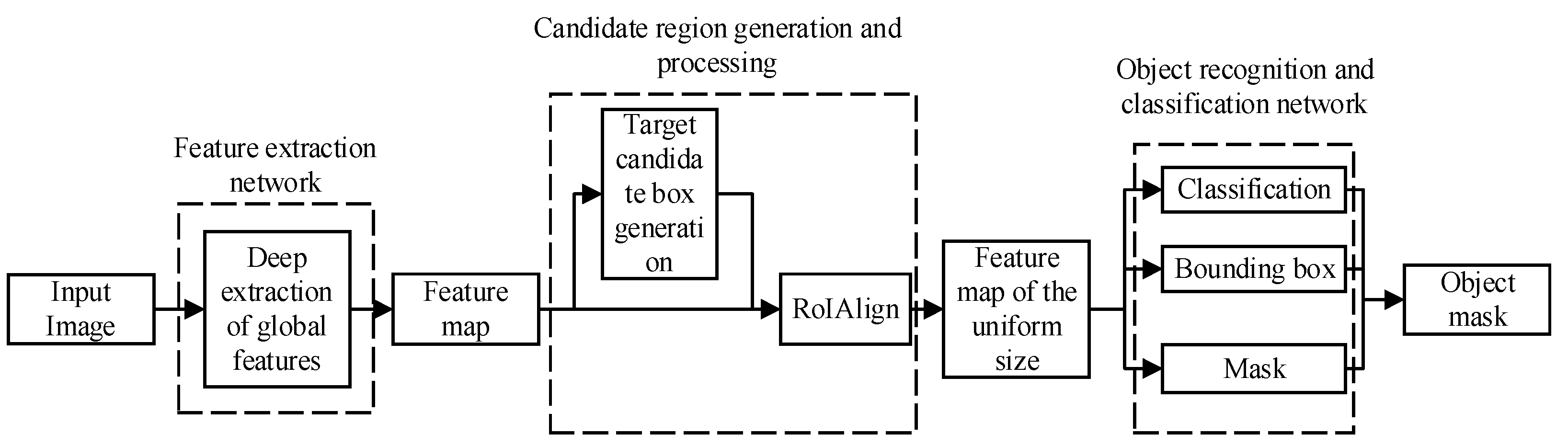
2.1. Feature Extraction Network Construction of Instance Segmentation Model for Generating Object Masks

The feature extraction network of the instance segmentation model for generating object masks is composed of the ResNet and the FPN (Figure 2). In Figure 2, the image of special-shaped sheet metal with multi-objective overlapping is input into the ResNet, and the ResNet divides the image into five levels {C1, C2, C3, C4, C5} from the bottom up. The length and width of the feature map of each level are 0.5 times the size of the feature map in the previous level. The five-level feature pyramid can effectively extract the feature information of targets of different scales and can provide enough multi-scale information to process objects of different sizes, so as to achieve high detection and segmentation accuracy while maintaining a certain computational efficiency.

After conducting a 1 × 1 convolution, the topmost C5 feature layer builds the top-down FPN network {M5, M4, M3, M2}. Then the topmost M5 performs upsampling. After expanding the length and width of the M5 to twice its original size, it is added to the feature map of the ResNet C4 via a 1 × 1 convolution to generate the M4. The M4 is then processed with a 3 × 3 convolution to generate the P4 feature map, and this fused feature map is then output for use in the reset of the entire feature extraction network. In this way, the four fused feature maps of {P2, P3, P4, P5} at different scales are generated. Additionally, P6 is generated by applying max pooling to P5 and is primarily utilized for subsequent network training.

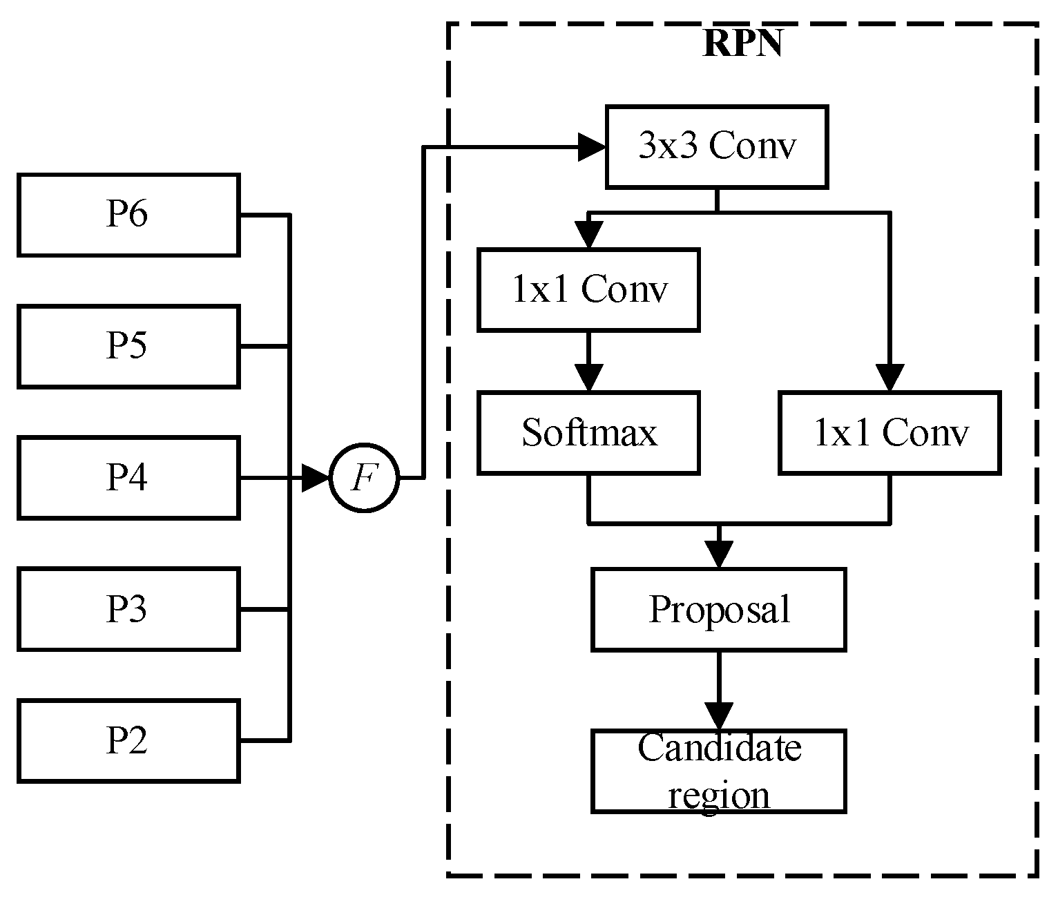
2.2. Feature Map Candidate Region Generation Network

Once the feature extraction network produces feature maps of different scales, namely {P2, P3, P4, P5, and P6}, these feature maps are passed to the RPN for region segmentation, generating detection anchor frames that encompass the objects. Figure 3 shows the network structure of the RPN, where $F$ is the judgment function. After generating the feature maps {P2, P3, P4, P5, P6} fused at various levels through the feature extraction network in Figure 2, $F$ was used to determine which level of the feature map was input into the RPN.

Assume that $k_0$ denotes the feature map at a certain level; $w$ and $h$ represent the length and width of the object’s candidate frame, i.e., the region of interest (ROI), after the feature map is convolved by the RPN; and $l_0$ denotes the size of the pre-trained dataset image. Then $F$ is expressed as follows:

$$F=\left[k_0+{\log }_2\left(\sqrt{wh}/l_0\right)\right]$$

(1)

where the default value of $k_0$ is 4, which means that the feature map of the fourth level is selected, and $l_0$ is generally set to 224 [18]. When the size of the ROI is less than 224, the calculation result will be less than 4, indicating that a low-level and high-resolution feature map shall be selected. In this way, it can expand the range of the feature extraction, which is conducive to detecting small objects. When the size of the ROI is greater than 224, it means that a high-level and low-resolution feature map shall be selected to refine the features and help detect large objects.

In Figure 3, after the selected feature map is input into the RPN, each pixel of the feature map generates nine types of anchor frames with three shapes and three length/width ratios. Firstly, these anchor frames will go through a 3 × 3 convolution and be divided into two branches. The anchor frames in the first branch will obtain two scores each after being processed with a 1 × 1 convolution and SoftMax, and these two scores are the probability of classifying the anchor frame as the foreground or background. The anchor frames in the second branch undergo a 1 × 1 convolution to correct the coordinates of the four points of each anchor frame so that the boundaries of the candidate frames will be classified as the foreground more accurately. After processing the two branches, a host of candidate regions containing objects were obtained. However, these candidate frames contained duplicate regions, and the direct operation might result in duplicate operations. Therefore, the information processed by the above two branches was input into the proposal layer to reduce the amount of computation and make the final prediction more accurate. In the proposal layer, we sorted the confidence of the foreground candidate frames, removed those with low confidence, and discarded those with a size less than the threshold value. We removed the candidate boxes that partially overlapped with the candidate box with the highest confidence, and the coincidence degree was higher than the threshold value via non-maximum suppression [20,21].

After generating the target candidate frame, we input the feature map to the subsequent network after converting it to the uniform fixed size using a bilinear interpolation through the Region of Interest Alignment (RoIAlign) module (see Figure 1) [2].

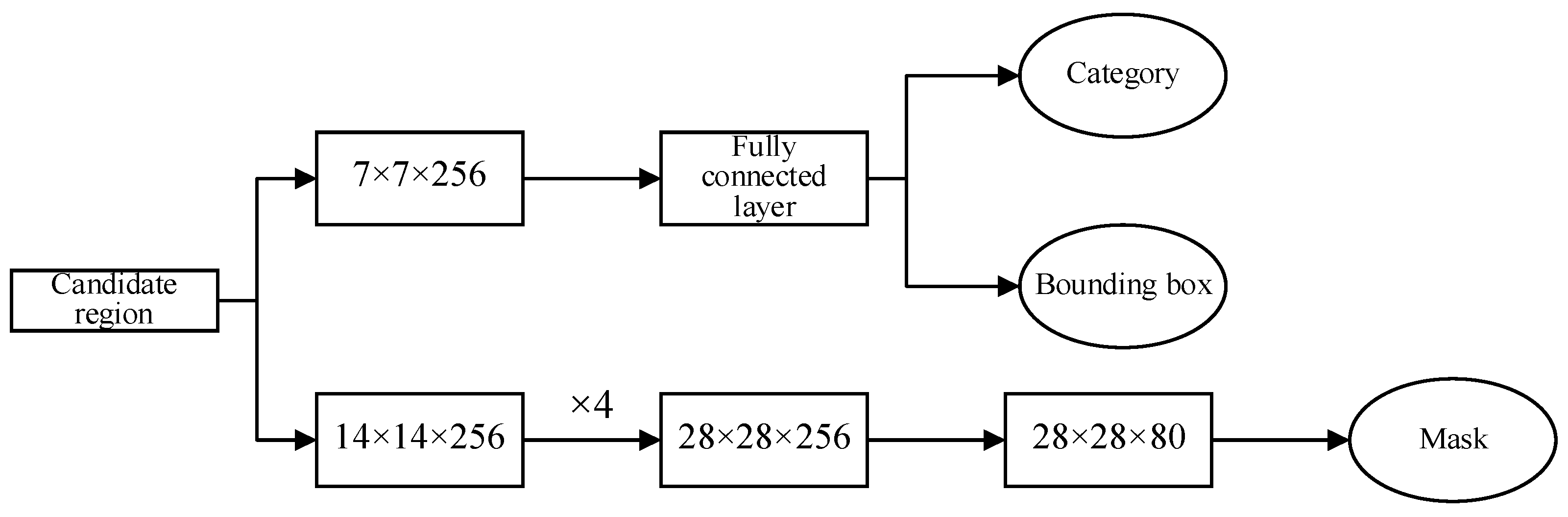
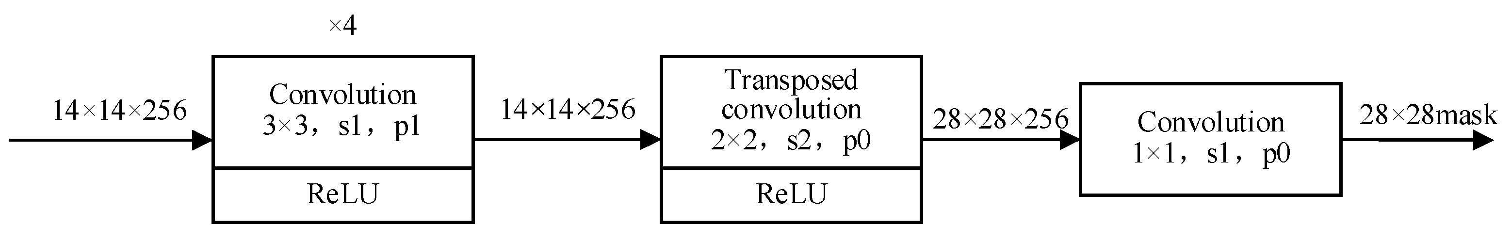
2.3. Object Recognition and Classification Network

It can be seen from Figure 4 that the feature maps with a uniform size are input into the object recognition and classification network after being processed by the RoIAlign module. The object recognition and classification network has three branches. Branch 1 is to classify the object category, Branch 2 is to perform the object bounding box regression, and Branch 3 is to generate the object mask. As shown in Figure 4, in Branch 1 and Branch 2, the feature map first undergoes a 7 × 7 convolutional layer and then is input into the fully connected layer to obtain the specific predicted category and bounding box position information. In Branch 3, to obtain higher segmentation accuracy, it is necessary to retain more segmentation details, so the feature map is pooled to a size of 14 × 14. Compared with the 7 × 7 feature map of Branch 2, it has more detailed information to obtain better results. Figure 5 shows the specific process of mask segmentation. The 14 × 14 feature map undergoes four 3 × 3 convolutions and rectified linear (ReLU) activation functions and then undergoes a 2 × 2 transposed convolution and ReLU activation functions. After that, upsampling is performed to obtain a 28 × 28 feature map, and finally, a 1 × 1 convolution is conducted to obtain a mask with a uniform size of 28 × 28.

During training, the mask segmentation model must undergo many iterations to achieve a high level of precision. As the model will be optimized by gradient descent through backpropagation, a loss function needs to be constructed for the training of the model.

The object recognition and classification network shown in Figure 4 contains the object classification, bounding box regression, and object mask. Assume that $L{F}_{cls}$ denotes the classification loss of the object category, which is used to judge the possibility of a certain category; $L{F}_{box}$ denotes the loss of the bounding box, which is used to measure the deviation of the candidate frame from the real position; and $L{F}_{mask}$ denotes the mask loss, which corresponds to the pixel-level task. After calculating the exact location of the object, we evaluated each pixel to determine whether it was the background or an object and then compared it with the real situation of the image to obtain the mask loss value. Finally, $LF$ denotes the total loss function, as shown in Formula(2) [22].

$$LF=L{F}_{cls}+L{F}_{box}+L{F}_{\mathrm{mask} }$$

(2)

Specifically, in terms of the object category classification branch, the output is the probability of the object classification. Assume that X and Y denote the input variable and output variable, respectively, $x_i$ represents the $i$th sample of $X$, and $y_j$ represents the jth sample of $Y$; $M$ and $N$ represent the number of output categories and the total samples, respectively; $k$ represents the $k$th category in the object category; and $q_{ik}$ indicates whether the current category $k$ is the category of the current input $x_i$, that is, whether the category classification prediction is correct. If so, it indicates that the value of the loss function is 1; otherwise, it is 0. $p_{ik}$ denotes the probability that the current input $x_i$ belongs to category $k$ after the network prediction. Then the classification loss function of the object category represented by the cross entropy is shown in Formula (3).

$$L{F}_{cls}\left(Y,P\left(Y\mid X\right)\right)=-\log P\left(Y\mid X\right)=-\frac{1}{N}{\sum }_{i=1}^N{\sum }_{k=1}^M{q}_{ik}\log \left(p_{ik}\right)$$

(3)

For the position coordinate value of the bounding box predicted by the bounding box regression, the Smooth $L1$ loss is used as the loss function [23]. The definition of Smooth $L1$ is shown in Formula (4).

$$L_{\mathrm{box} }\left(t_i,t_i^{*}\right)=Smooth L1\left(t_i-t_i^{*}\right)\dots Smooth L1\left(x\right)=\{\begin{array}{cc}0.5x^2& x<1\\ \left|x\right|-0.5& x\ge 1\end{array}$$

(4)

where $t_i$ denotes the predicted coordinate parameter of the bounding box, while $t_i^{*}$ represents the actual coordinate parameter of the bounding box.

As for the loss function of the mask prediction branch, the mask prediction branch outputs mask images with a fixed size, so the average binary cross entropy is used to denote the loss function, as shown in Formula (5).

$$L{F}_{\mathrm{mask}}\left(b,o\right)=-\left(b·\log \left(o\right)+\left(1-b\right)·\log \left(1-o\right)\right)$$

(5)

where $b$ denotes the label, and $o$ denotes the actual model output.

In this way, we obtained the total loss function $LF$ of the object recognition and classification network, and the $LF$ was used as a standard to measure the performance of the model to generate object masks.

2.4. Model Calculation Complexity

The computational complexity of the model specifically refers to the time complexity and the space complexity. The time complexity determines the training and prediction time of the model, and the space complexity determines the number of parameters of the model. In this paper, the multi-objective overlapping metal thin part case segmentation model is composed of three parts, which are the feature extraction network of the global feature deep-level extraction, the RPN network of the target candidate region, and the target recognition classification network.

In order to effectively reduce the computational complexity of the model, as shown in Figure 2, we added a maximum pooling layer after the P5 layer for the pooling operation, so that the output P6 feature map size became smaller and the data volume was reduced to reduce the time complexity of the model. As shown in Figure 4, in order to reduce the spatial complexity of the model and ensure that the model has a high segmentation accuracy, we pooled the feature map to a size of 14 × 14 in the mask prediction branch, and the number of channels of the input feature map was reduced from 256 to 80, effectively reducing the spatial complexity of the model.

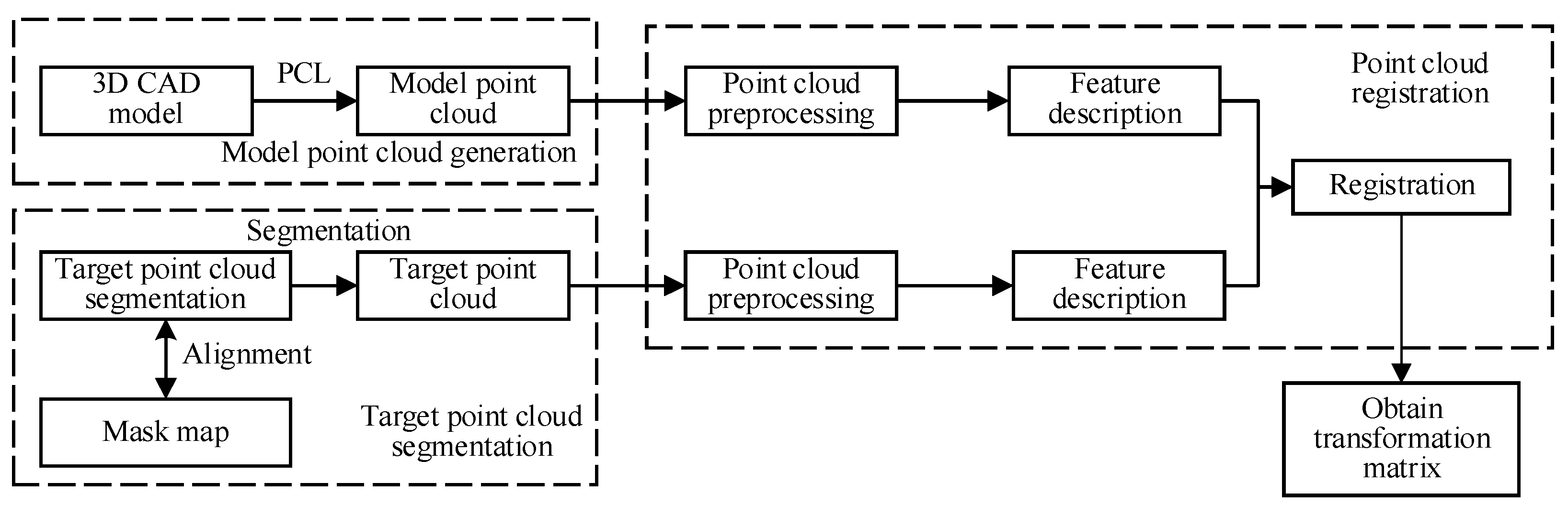
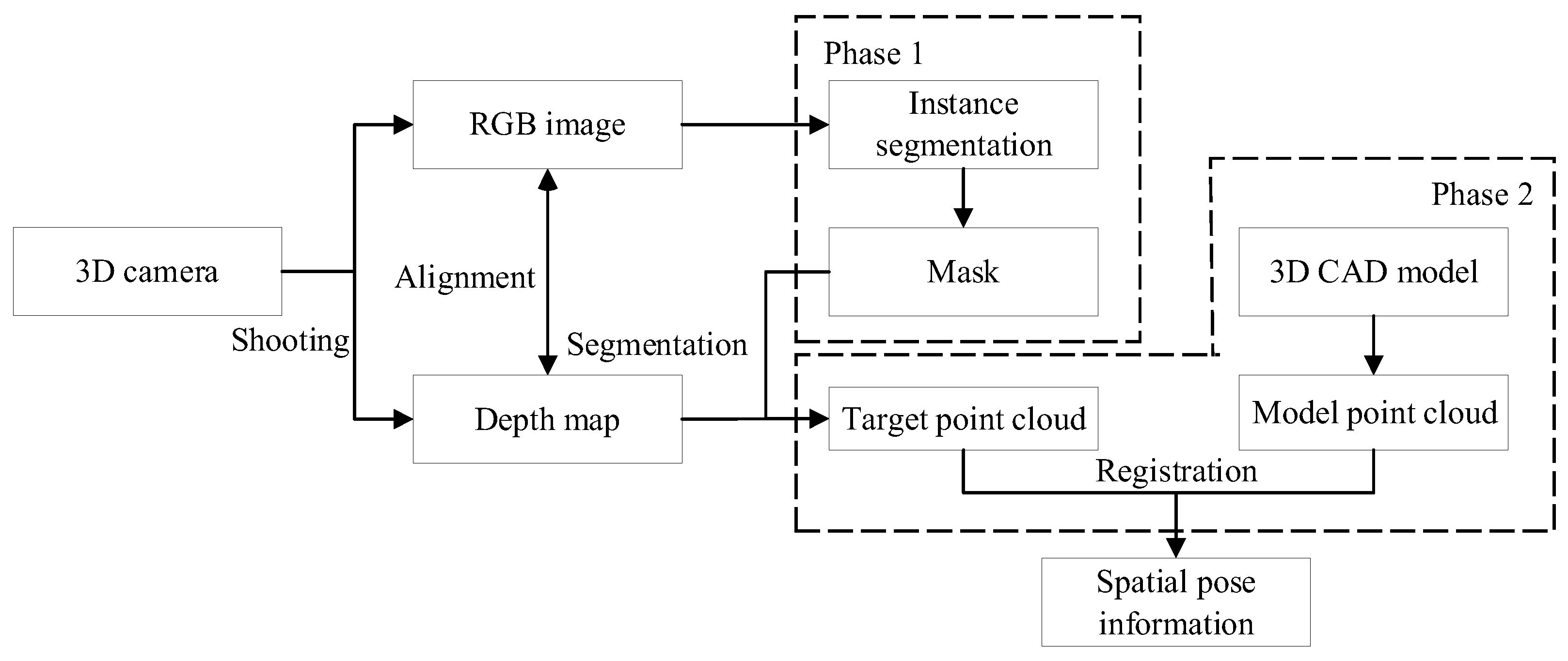
3. Pose Estimation Method of Metal Deformed Thin Parts Based on 3D Point Cloud

We obtained the object mask information of special-shaped sheet metal via instance segmentation. To realize the pose estimation of special-shaped sheet metal, it is necessary to generate the target point cloud of special-shaped sheet metal and register it with its model point cloud to obtain the actual pose information. The principle of the pose estimation method for special-shaped sheet metal based on a 3D point cloud is shown in Figure 6. In this figure, the point cloud segmentation of the target object can be realized by aligning the object mask with the depth map [24] to obtain the target point cloud of the single special-shaped sheet metal. The model point cloud can convert the 3D model of SolidWorks into point cloud data with the point cloud library (PCL), thus obtaining the model point cloud data [25]. The point cloud registration module performs downsampling on the target point cloud and the model point cloud using a VoxelGrid filter to reduce the density of the point cloud and improve the calculation efficiency, and then it calculates the fast point feature histogram (FPFH) local feature descriptor and uses the sample consensus initial alignment algorithm (SAC-IA) for coarse registration and the iterative closest point (ICP) algorithm [26] for fine registration.

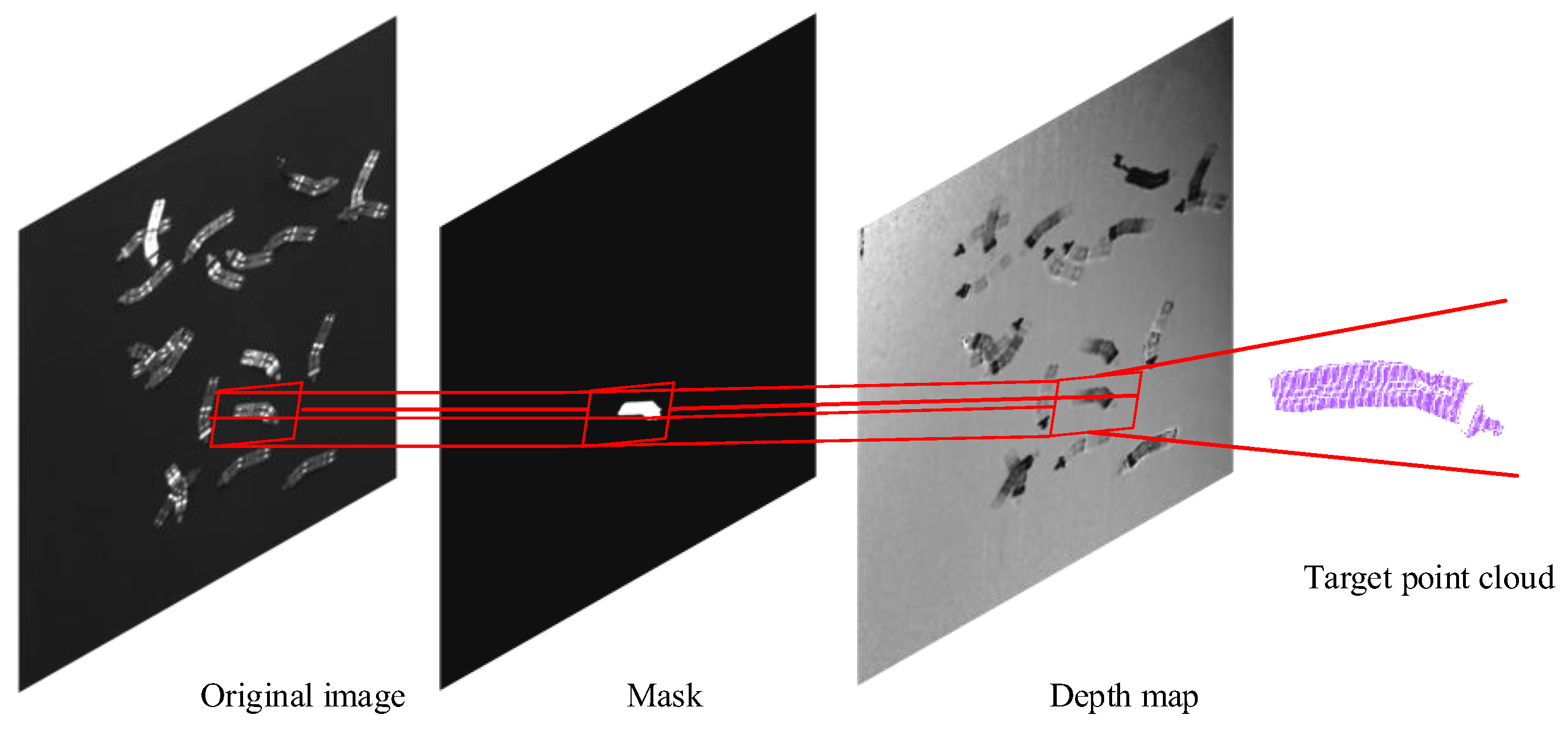
3.1. Target Point Cloud Segmentation and Model Point Cloud Generation

In the preceding section, the target mask information is derived through an example of 2D-pixel-map-based segmentation. As the 2D pixel map and depth map are appropriately aligned, the alignment of the target mask and depth map is also ensured. The object can be segmented from the depth map by the mask image, and then the 3D coordinates of each pixel can be calculated by the internal and external parameters of the depth camera to obtain the target point cloud [27].

Assume that $p=\left[C_x,C_y\right]$ is a pixel in the object mask image, which corresponds to the point $P=\left[P_x,P_y,P_z\right]$ in 3D coordinates; $u$ and $v$ denote the center coordinates of the mask image; $dx$ and $dy$ represent the metric relationship between image coordinates and pixel coordinates; $f$ denotes the focal length of the camera; $d$ denotes the Z-axis value of the camera coordinates (that is, the distance from the object to the camera); and $R$ and $T$ denote the 3 × 3 rotation matrix and 3 × 1 translation matrix of the extrinsic matrix, respectively. Then, $p=\left[C_x,C_y\right]$ and $P=\left[P_x,P_y,P_z\right]$ satisfy the calibration relationship shown in Formula (6) [28].

$$d\left(\begin{array}{c}{C}_x\\ C_y\\ 1\end{array}\right)=\left[\begin{array}{ccc}f/dx& 0& u\\ 0& f/dy& v\\ 0& 0& 1\end{array}\right]\left[\begin{array}{cc}R& T\end{array}\right]\left[\begin{array}{c}{P}_x\\ P_y\\ P_z\\ 1\end{array}\right]$$

(6)

Given that the mask map and depth map are aligned, implying the absence of rotation and translation, the rotation matrix $R$ and translation matrix $T$ can be represented by Formula (7).

$$R=\left[\begin{array}{ccc}1& 0& 0\\ 0& 1& 0\\ 0& 0& 1\end{array}\right],T=\left[\begin{array}{c}0\\ 0\\ 0\end{array}\right]$$

(7)

By substituting Formula (6) into Formula (5) and simplifying the expression, we obtain the transformation formula from the mask pixel point $\left[C_x,C_y\right]$ $T$ to the 3D coordinate point $\left[P_x,P_y,P_z\right]$ $T$, as shown in Formula (8).

$$\{\begin{array}{c}{P}_z=d\\ P_x=\left(c_x-u\right)\times P_z\times d_x/f\\ P_y=\left(c_y-v\right)\times P_z\times d_y/f\end{array}$$

(8)

Formulas (6)–(8) show the calculation process of the 3D coordinates of each pixel in the object mask image. By calculating the 3D coordinates of each pixel of the target mask image based on Formula (8), we obtained the target point cloud data.

As for the model point cloud generation method, given that the special-shaped sheet metal is manufactured in batches by high-precision molds, the size error is small, and the 3D model of special-shaped sheet metal can be used to generate point clouds. Our approach is to employ the SolidWorks software to export the 3D model in the format of standard triangle language (STL), then adopt the PCL software to open the STL file and convert it into a PLY file, and finally save it in the PCD point cloud format.

To enhance the efficiency and accuracy of subsequent point cloud registration, downsampling is recommended for both the acquired target point cloud and model point cloud data. This downsampling process aims to reduce the number of points while preserving the original appearance and features of the point clouds. In this study, we proposed to achieve this process by performing downsampling on the point cloud using a VoxelGrid filter [29]. The specific steps are as follows. First, we created a 3D voxel grid for the processed point cloud data, divided the created voxel grid into several small grids according to certain criteria, obtained the density center position inside each small grid, and calculated the distance between the points inside each small grid and the density center. Finally, we removed the points that did not meet the distance requirements to perform downsampling on the point cloud. The specific steps are as follows:

Step 1: Use Formula (9) to determine the side length $L$ of the small cubic grid.

$$L=\alpha \sqrt[3]{\frac{s}{g}}$$

(9)

where $s$ denotes the scale factor, $g$ denotes the regulatory factor, the value of $\alpha$ is regulated based on the scale of the input point cloud data, and $g$ denotes the number of points in the small grid and is calculated by Formula (10).

$$g=\sqrt{\frac{N}{V}}$$

(10)

where $N$ denotes the number of all points inside the point cloud, and $V$ denotes the maximum volume of the external voxel grid of the point cloud. The definition of $V$ is shown in Formula (11).

$$V=L_x{L}_y{L}_z$$

(11)

where $L_x$, $L_y$, and $L_z$ respectively denote the maximum length of the external voxel grid in the directions of the $x$ -axis, $y$ -axis, and $z$ -axis. Additionally, to ensure that all point cloud data are in the external voxel grid, it is necessary to add $\lambda$ appropriately in each direction to increase the length of each direction, as shown in Formula (12).

$$\{\begin{array}{c}{L}_x=\left(x_{\max }-x_{\min }\right)+\lambda \\ L_y=\left(y_{\max }-y_{\min }\right)+\lambda \\ L_z=\left(y_{\max }-y_{\min }\right)+\lambda \end{array}$$

(12)

By substituting Formulas (10) and (11) into Formula (9), we can obtain the size of $L$ (see Formula (13)).

$$L=\alpha \sqrt[3]{\frac{s{L}_x{L}_y{L}_z}{N}}$$

(13)

It can be seen from Formula (13) that the size of $L$ is related to the average density of the input point cloud.

Step 2: According to the side length $L$, divide the external voxel grid into $m\times n\times 1$ small cubic grids (see Formula (14)).

$$\{\begin{array}{c}m=\mathrm{ceil}\left(L_x/L\right)\\ n=\mathrm{ceil}\left(L_y/L\right)\\ l=\mathrm{ceil}\left(L_z/L\right)\end{array}$$

(14)

where $\mathrm{ceil}\left(x\right)$ denotes the smallest integer not less than $x$. For any point $p$ in the point cloud, its corresponding grid code is $(m_p,n_p,l_p)$, which is calculated by Formula (15).

$$\{\begin{array}{c}{m}_p=\mathrm{ceil}\left(\left(x_p-x_{\min }\right)/L\right)\\ n_p=\mathrm{ceil}\left(\left(y_p-y_{\min }\right)/L\right)\\ l_p=\mathrm{ceil}\left(\left(z_p-z_{\min }\right)/L\right)\end{array}$$

(15)

Step 3: After calculating the grid coding of each point according to Formula (15), calculate the density center of the 3D grid (see Formula (16)).

$$\{\begin{array}{c}{X}_{ci}={\displaystyle \sum _{i=1}^g}{x}_i/g\\ Y_{ci}={\displaystyle \sum _{i=1}^g}{y}_i/g\\ Z_{ci}={\displaystyle \sum _{i=1}^g}{z}_i/g\end{array}$$

(16)

where $g$ denotes the number of point clouds in each small cubic grid. Based on the distance from each point (see Formula (15)) in the grid to the corresponding density center (see Formula (16)), we retain or remove points to perform the downsampling.

3.2. Registration of Target Point Cloud and Model Point Cloud

In Figure 6, which was mentioned in the previous section, after generating the model point cloud and the target point cloud, the characteristics of the two types of point cloud data need to be described before the point cloud registration.

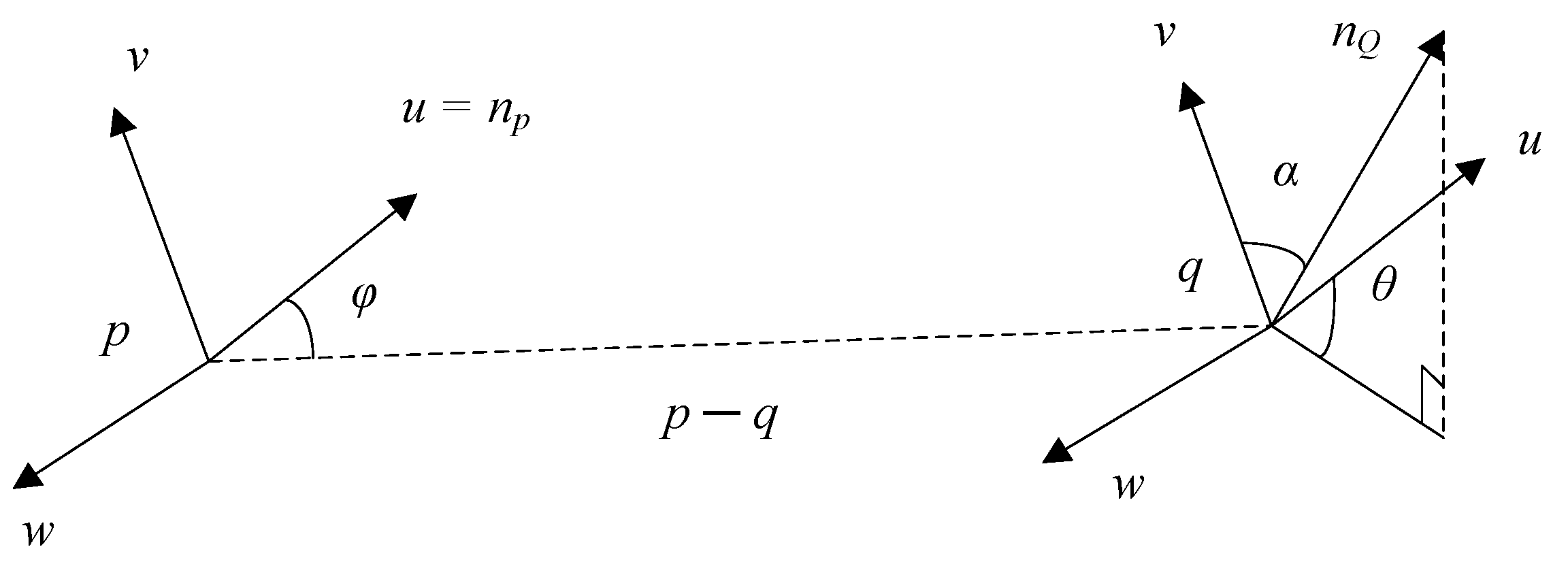
3.2.1. Establish Point Cloud Feature Descriptor

Point cloud feature description plays a vital role in point cloud registration tasks. For point cloud data in 3D space, we used the vector or matrix to describe the interrelationship between a point feature and its neighboring point clouds and then characterized the similarity of different point clouds by this relationship. This process is called point cloud recognition, and the vector or matrix describing this relationship is called the feature descriptor [30]. A point cloud feature descriptor can be divided into global feature descriptors and local feature descriptors by scale. The former is the feature set formed by encoding the overall geometric features of the point cloud, and the latter is based on geometric features such as neighborhood normal vectors. Compared with the global feature descriptor, the local feature descriptor has a higher fault tolerance and is less subject to point cloud rotation and density reduction.

A fast point feature histogram (FPFH) [31] is an improvement of a point feature histogram (PFH) [32]. The idea of it is to form specific parameters to describe the changes in the object surface by parameterizing the interaction between the normal features of a point in the point cloud and the normal vector of its neighboring points. A FPFH can lower the computational complexity. Assuming that there are n points in a point cloud, and $k$ denotes the number of points in the neighborhood of the sample point in this point cloud, the theoretical computational complexity of PFH is O ($n{k}^2$). The FPFH feature descriptor lowers the complexity to O ($nk$) while retaining most of the PFH recognition effects, effectively reducing the computation time.

In the FPFH feature descriptor, to represent the interaction between the normal of a point $p$ in the point cloud and the normal of a point $q$ in its neighborhood, $n_p$ denotes the normal vector of the point $p$, $n_Q$ denotes the normal vector of the point $q$, $\alpha$, $\phi$, and $\theta$ denote the normal deviation (see Figure 7), and the $uwv$ local coordinate system is constructed with $p$ as in Formula (17).

$$\{\begin{array}{c}u=n_p\\ v=\left(p-q\right)\times u\\ w=u\times v\end{array}$$

(17)

Furthermore, the interaction of the normal between $p$ and $q$ is described in Formulas (18)–(20).

$$\alpha =v\cdot n_Q$$

(18)

$$\phi =\frac{u\cdot \left(p-q\right)}{\Vert p-q\Vert }$$

(19)

$$\theta =\arctan \left(w\cdot n_Q,u\cdot n_Q\right)$$

(20)

By placing the above three parameters into the histogram interval statistically, we can obtain the FPFH descriptor. The FPFH feature descriptor is calculated as follows:

Step 1: For a point $p$ in the point cloud, we only need to calculate the values of {$\alpha$, $\phi$, $\theta$}. Compared with a PFH, this step simplifies the relationship between neighborhood points, and the result is called the simplified point feature histogram (SPFH).

Step 2: ${\omega }_k$ denotes the distance between $p$ and its neighboring point $p^{\prime }$. Re-traverse the $k$ neighborhood of point $p^{\prime }$ to be queried in Step 1. According to the value of the SPFH between the two points, we can obtain the FPFH value of this point according to Formula (21).

$$FPFH\left(p\right)=SPFH\left(p\right)+\frac{1}{k}{\displaystyle \sum }_{i=1}^k\frac{1}{{\omega }_k}\cdot SPFH\left(p^{\prime }\right)$$

(21)

Compared with a PFH, the FPFH feature descriptor simplifies the calculation of the relationship between neighboring points and reduces the amount of calculation. Additionally, by taking the neighboring point as the center of $p^{\prime }$, we determine the SPFH value in the $k$ neighborhood. By weighing and summing the SPFH values of point $p$ and neighboring points $p^{\prime }$, we obtain the FPFH value at point $p$, which reduces the computational effort and enhances the information utilization of neighboring points.

3.2.2. Point Cloud Coarse Registration Algorithm

The template point cloud and the target point cloud in this study are not in the same coordinate system; the initial pose difference is too large, and the direct fine registration may obtain the local optimal solution, resulting in wrong results. Therefore, we usually perform coarse registration first to obtain appropriate initial values, making the two point clouds close to each other, and then conduct fine registration. The widely used coarse registration algorithms include the SAC-IA algorithm and the normal distribution transform (NDT) algorithm [33]. In this study, we explored these two coarse registrations separately and tested their accuracy and efficiency in registration between a model point cloud and a target point cloud of special-shaped sheet metal.

(1)

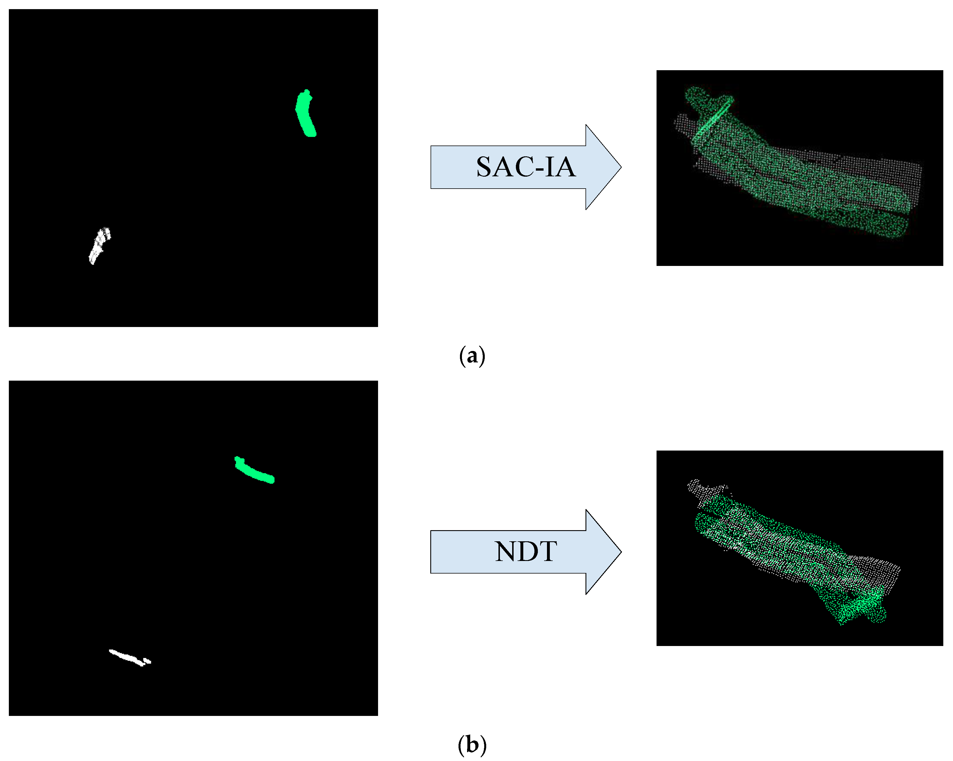
Coarse registration algorithm based on SAC-IA. Based on the FPFH feature descriptor, we searched the corresponding points in the point cloud and then used the sampling consistency to iterate continuously to remove the wrong corresponding points and solve the rigid transformation matrix with minimal registration errors. The specific implementation steps are as follows.

Step 1: Select n sampling points from the target point cloud set P. The distance between sampling points shall be greater than the preset threshold d to avoid a situation in which the FPFH feature descriptors of the selected sampling points are similar.

Step 2: Find one or more points in the template point cloud set Q that have similar FPFH characteristics to the sample points in the target point cloud set P. Randomly select a set of corresponding points from these similar points.

Step 3: Calculate the rotation and translation matrix between the corresponding points, and then use the Huber function to evaluate the matching quality of the matrix pose and the actual pose. The Huber penalty function is expressed as $\sum _{i=1}^{n}H\left(l_i\right)$:

$$H\left(l_i\right)=\{\begin{array}{cc}\frac{1}{2}{l}_i^2,& l_i<ml\\ \frac{1}{2}ml\left(2l_i-ml\right),& l_i>ml\end{array}$$

(22)

where $ml$ denotes the preset threshold value, and $l_i$ denotes the distance value of the corresponding point in the $i$th group.

Step 4: Repeat Steps 1–3 to find a set of optimal solutions. The transformation matrix of the optimal solution is the final registration result.

(2)

Coarse registration algorithm based on NDT. The NDT algorithm converts the solution of the rigid transformation matrix into the solution of the optimal value of the probability distribution function. In other words, it uses the continuously differentiable probability density function to describe the distribution of points in the point cloud and then solves the optimal solution of the likelihood function from the template point cloud to the target point cloud to obtain the transformation matrix. The specific steps are as follows:

Step 1: Divide the model point cloud space into several sub-voxel grids. Each voxel grid is composed of a point set ($x_i$, $y_i$, $z_i$). Calculate the covariance matrix $\Sigma$ and mean vector $\overrightarrow{{\mu }_{ı}}$ in each grid, as shown in Formulas (23) and (24):

$$\Sigma =\frac{1}{n-1}{\sum }_{i=1}^n\left(\overrightarrow{x_t}-\overrightarrow{{\mu }_t}\right){\left(\overrightarrow{x_{ı}}-\overrightarrow{{\mu }_{ı}}\right)}^T$$

(23)

$$\overrightarrow{{\mu }_{ı}}=\frac{1}{n}{\sum }_{i=1}^n\overrightarrow{x_i}$$

(24)

Step 2: Converse the template point cloud to the target point cloud coordinate system.

Step 3: Calculate the probability of conversion points falling within the corresponding voxel grid after coordinate transformation according to Formula (25):

$$p\left(x\right)~\exp \left(-\frac{{\left(\overrightarrow{x_{\mathrm{t}}}-\overrightarrow{{\mu }_{\mathrm{l}}}\right)}^T{\Sigma }^{-1}\left(\overrightarrow{x_{\mathrm{t}}}-\overrightarrow{{\mu }_{\mathrm{l}}}\right)}{2}\right)$$

(25)

Step 4: Count the probability of conversion points falling within the corresponding voxel grid and obtain the NDT registration $score$ by Formula (26).

$$score\left(p\right)={\sum }_i\exp \left(-\frac{{\left(\overrightarrow{x_{\mathrm{t}}}-\overrightarrow{{\mu }_{\mathrm{t}}}\right)}^T{\Sigma }^{-1}\left(\overrightarrow{x_{\mathrm{t}}}-\overrightarrow{{\mu }_{\mathrm{t}}}\right)}{2}\right)$$

(26)

Step 5: Use the Newton–Raphson method to perform constant iteration to obtain the maximum value of the $score\left(p\right)$ function.

3.2.3. Point Cloud Fine Registration Algorithm

After the coarse registration in the previous step, the model point cloud and the target point cloud have nearly overlapped. In the next step, the fine registration algorithm will be performed for further registration. The ICP algorithm [34] employs Euclidean distance to measure whether it is a corresponding point, establishes a set of corresponding points, and then uses the rigid transformation matrix method to solve the transformation matrix between the corresponding points. The point cloud data are iteratively updated until the mean square error between the correspondence points is less than the set threshold, or it reaches the maximum number of iterations. The result of the last iteration is the registration result. The specific steps are as follows:

Step 1: For a point $p_i$ in the model point cloud $P$, find the point $q_i$ closest to its Euclidean distance in the target point cloud $Q$ to form a corresponding point set;

Step 2: Calculate the normal vector angle ${\theta }_i$ of each corresponding point pair. If ${\theta }_i$ is greater than the set threshold $\beta$, remove the corresponding point pair;

Step 3: Calculate the transformation matrix of each corresponding point pair to minimize the registration error $f\left(R,T\right)$:

$$f\left(R,T\right)=\frac{1}{n}{\sum }_{i=1}^n\Vert p_i-{\left(R{q}_i+T\right)\Vert }^2$$

(27)

Step 4: Apply the obtained transformation matrix to the target point cloud $Q$ to obtain a new target point cloud $Q^{\prime }$:

$$Q^{\prime }=R\cdot Q+T$$

(28)

Step 5: Calculate the mean square error ${\epsilon }_k$ of the corresponding point pair after iteration:

$${\epsilon }_k=\frac{1}{n}{\sum }_{i=1}^n{p}_i-q_i{}^2$$

(29)

Step 6: If ${\epsilon }_k$ < $\epsilon$ or $k$ > $k_{max}$, the iteration stops; otherwise, repeat Steps 1–5;

Step 7: Take the result of the last iteration as the final registration result.

As the ICP algorithm is based on point cloud rotation and translation, it will consume a lot of time and computational resources in the early iteration when using Euclidean distance to find the corresponding points for two sets of point clouds with different initial pose distances. If you start with the matrix iteration rotation and translation in a direction that satisfies the threshold value, it may get trapped into local optima, resulting in a false match. Therefore, coarse registration is usually added before ICP registration to narrow the difference in the viewing angle between the two point clouds and make the two point clouds close to each other before using ICP fine registration algorithm. In this way, we can obtain better registration results.

Given the main difficulties in the 3D pose estimation of special-shaped sheet metal, we elaborated on the ideas and methods of object mask generation, target point cloud segmentation and model point cloud generation, and target point cloud and model point cloud registration based on instance segmentation. Furthermore, we deduced the corresponding calculation formula and introduced the algorithm steps. In the following, the above algorithm will be validated and tested in conjunction with the 3D pose recognition of thin special-shaped sheet metal in an actual assembly.

4. Experimental Verification and Testing

To verify the effectiveness of the above method, we adopted special-shaped nickel sheets commonly used in the assembly of new energy batteries as the experimental object (see Figure 8a).

Sheet metal is thin, has a non-symmetrical shape with positive and negative sides, and is easy to deform. During the assembly process, nickel sheets are often scattered and disordered in the material frame. There may be an occlusion between nickel sheets, so it is necessary to consider this factor (see Figure 8b). Moreover, due to the overlapping issue, the height information of nickel sheets in the material frame is unknown. Commonly, plane picking may cause nickel sheet deformation and damage the end effector of the manipulator. To pick up the nickel sheet accurately, it is necessary to obtain the spatial pose information of the nickel sheets in the material frame. Our spatial pose recognition experiment on nickel sheets mainly includes two stages (see Figure 9). In the first stage, the instance segmentation model proposed in this study was used to detect the nickel sheets and obtain the corresponding confidence scores, bounding box values, and masks. In the second stage, the pose estimation of the target nickel sheets was performed. The target point cloud was generated based on the mask information in the first stage and the depth map, and the spatial pose information of the target’s thin special-shaped part in the material frame was obtained using the model-based point cloud registration.

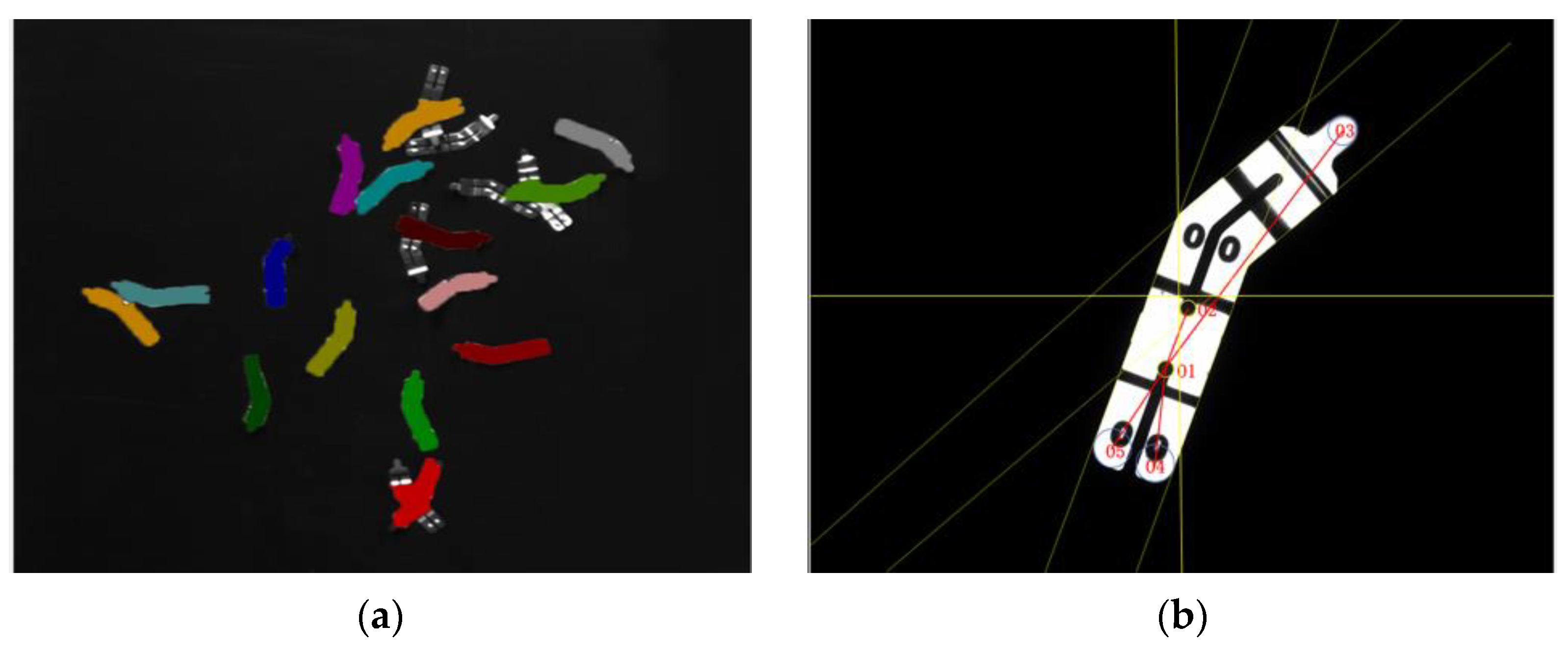
4.1. Instance Segmentation Experiment and Analysis

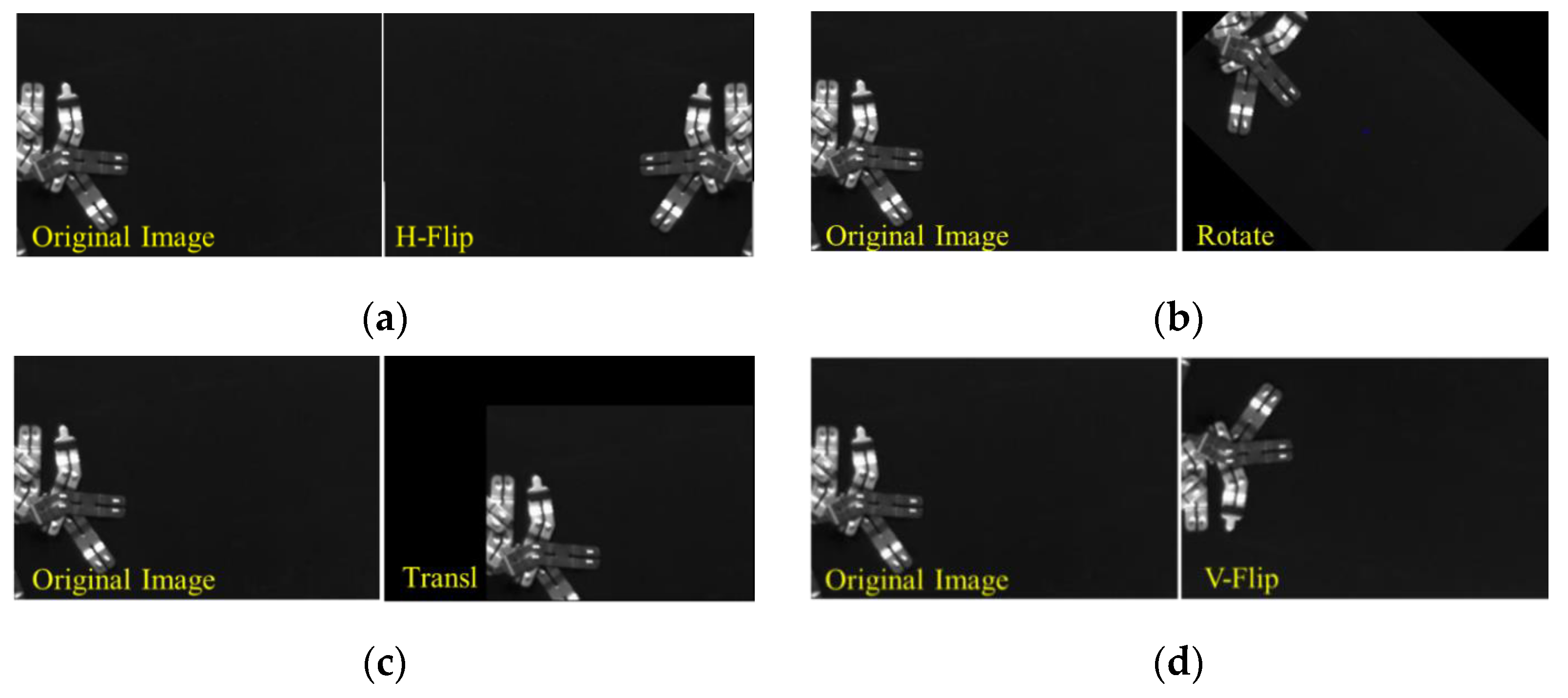
4.1.1. Custom Data Set Building

We employed a 3D high-definition and high-speed camera to acquire images with a resolution of 1080 × 980 in the target area, and then cropped each image to a small size of 360 × 240. This method not only reduced the label processing time, but also expanded the data samples. A total of 865 images of a size of 360 × 240 were obtained [35]. In this method, when we need to test large-sized images later, we just need to ensure the consistency of the scale of the images, crop them into the specified small-sized images in the same way, and then input them into the model for testing.

By enhancing the generalization capability of the model, we increased the number of images in the dataset while preventing the model from overfitting. We increased the number of images to 227 by data enhancement, such as flips, rotations, panning, and mirroring. Figure 10 shows renderings of our data enhancement methods, such as flips (a), rotations (b), translations (c), and mirroring (d), respectively.

Based on the image label definition rules, we divided the nickel sheets into Areas I, II, III, and IV. Specifically, Area I is the suction area of the manipulator end effector, and Areas II, III, and IV are the areas for judging the front and back of the nickel sheets (see Figure 11). According to the principle of the manipulator for picking up nickel sheets, when Area I is not occluded, the manipulator can pick up the target parts normally. Therefore, it is necessary to make labels according to the occlusion conditions of I, II, III, and IV.

Given the time-consuming nature of instance segmentation and labeling as well as the strategy of picking up nickel sheets by the manipulator, we explored the two types of labels, face up and face down, to reduce the time of manual labeling. Figure 12 shows the relevant schematic diagram.

In this study, we selected the powerful and convenient Labelme as the labeling tool for the dataset. In the labeling process, the face-up label was marked as fs. For different instances of the same type, they were denoted as fs1, fs2, fs3, etc. The face-down label was marked as fs. For different instances of the same type, they were denoted as bs1, bs2, bs3, etc.

After labeling all the images, we performed batch processing. Each image generated a folder containing label data. A total of 4091 objects in 1052 images were labeled, of which 2124 were face-up objects and 1967 were face-up objects. They constituted the dataset for this experiment.

4.1.2. Model Training Details Settings

The experimental conditions are configured as follows: the model is trained based on the TensorFlow framework. The software and hardware environment are configured as follows: TensorFlow version 1.14.0, Keras library version 2.1.6, and Python version 3.6.13. The hardware configuration is as follows: 64-bit Windows 10, Intel i7 10700, NVIDIA GTX-2080Ti 11 G video memory, and 32 GB memory. The model training parameters are set as shown in

Table 1. Main training parameters.

Name	Numeric Value	Description
backbone	ResNet + FPN	backbone network
image_per_gpu	1	number of images per load
learning_momentum	0.9	learning momentum
learning_rate	0.001	learning rate
weight decay	0.0001	learning rate decay
steps_per_epoch	700	steps per time
epoch	230	number of sample traversals
mask_shape	[28, 28]	mask size
rpn_train_anchors_per_image	256	number of bounding boxes

. These parameters are the hyperparameters of the model, which are the optimal hyperparameters obtained through multiple experiments and tuning to achieve the optimal performance of the model. Among them, the maximum number of iterations of model training is based on the evaluation index mAP_0.5, that is, when IOU = 0.5 and mAP_0.5 no longer rises, the obtained number of iterations is the maximum number of iterations of the model. Specifically, the backbone network is ResNet50 + FPN or ResNet101+ FPN, the GPU loads one image each time, the learning momentum is 0.9, the learning rate is 0.001, the learning rate decay is 0.0001, the number of steps per time is set to 700, the number of sample traversals is 230, the mask size is set to [28, 28], and the number of area bounding boxes is set to 256. The self-made dataset has 1052 labeled images, with 70% of them used as the training set, 20% as the validation set, and the rest as the test set.

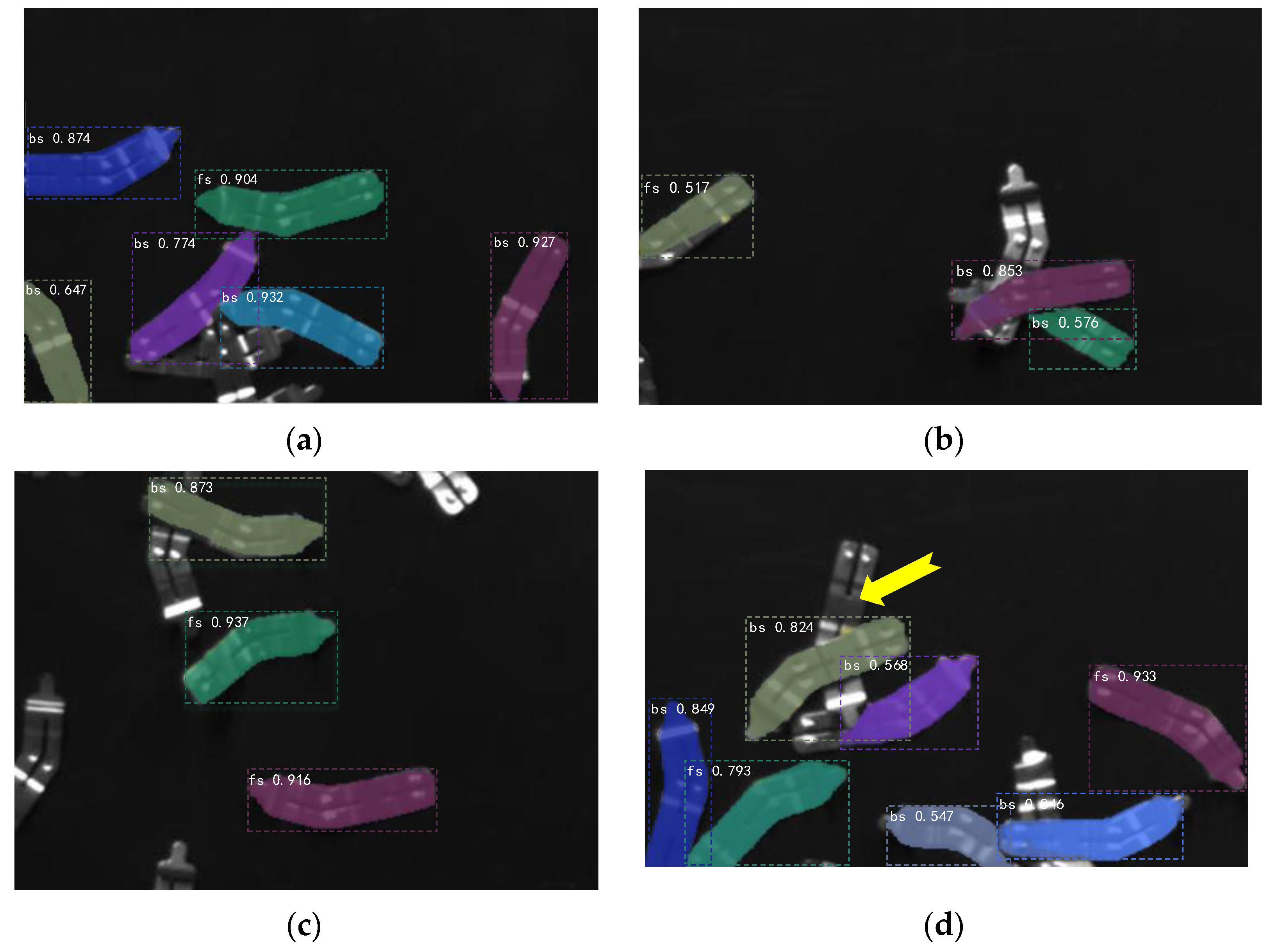
4.1.3. Experimental Results and Evaluation Analysis

We employed the test set in the custom dataset to test the performance of the model and adopted the ResNet50 + FPN and ResNet101 + FPN backbone networks to perform instance segmentation experiments [18]. Average precision (AP) was used to evaluate the model performance of instance segmentation. The size of AP is the area formed by the precision and recall curves and the X-axis. The higher the AP value, the better the performance of the model. The experimental results are shown in

Table 2. Comparison of AP_0.5 values of different backbone networks.

Backbone Network	AP0.5 Value of Front Side	AP0.5 Value of Reverse Side	mAP0.5
ResNet50 + FPN	97.6%	96.8%	97.2%
ResNet101 + FPN	97.8%	97.2%	97.5%

. In the case that IOU = 0.5, the detection results of the instance segmentation model based on ResNet50 + FPN showed an AP_0.5 value of 97.6% for the front side of the nickel sheet and 96.4% for the back side of the nickel sheet. The detection results of the instance segmentation model based on ResNet101 + FPN showed an AP_0.5 value of 97.8% for the front side of the nickel sheet and 97.2% for the back side of the nickel sheet.

In GPU mode, the time consumed by the two models with different backbone networks to test sizes of 360 × 240 and 1080 × 980 is shown in

Table 3. Time consumed by testing images of different sizes.

Backbone Network	360 × 240	1080 × 980
ResNet50 + FPN	0.617 s	1.563 s
ResNet101 + FPN	1.236 s	3.291 s

.

According to the comparison of experimental results of two different backbone networks, the mean average precision (mAP_0.5) based on ResNet101 + FPN is 97. 5%, and the mAP_0.5 based on ResNet50 + FPN is 97.2%. Moreover, the time consumed by testing an image based on ResNet50 + FPN is more than 50% less than that based on ResNet101 + FPN. In the assembly line of nickel sheets, efficiency is an important indicator, so it is reasonable to select the instance segmentation model based on ResNet50 + FPN.

We adopted the instance segmentation model based on ResNet50 + FPN to test the segmentation effect of four types of nickel sheets with different occlusion conditions. The segmentation results are shown in Figure 13. The nickel sheets that are not occluded in Figure 13a can be accurately segmented. In Figure 13b,c, the occluded nickel sheet in Area I (as indicated in Figure 11) was not divided as expected.

In Figure 13d, Areas I and III of the nickel sheets indicated by the yellow arrow are not occluded and belong to the positive samples, but they are not recognized. The main reason for this is that the nickel sheet not recognized by Figure 13d is occluded. The occluded nickel sheet and the nickel sheet piece covering it generate multiple candidate frames with the same label. In the NMS processing stage, only the candidate frames with intersection-over-union (IoU) scores lower than those of the set threshold were retained. The candidate frames with IoU scores higher than those of the set threshold were considered duplicates and removed, resulting in the occluded sheet metal being unrecognized.

According to the pick-up strategy of the manipulator, it tends to give priority to picking up the upper layer of the nickel sheet. When the upper layer of nickel metal is picked up, we can obtain more information about the nickel sheet pointed out by the yellow arrow, thus increasing the probability of being correctly recognized.

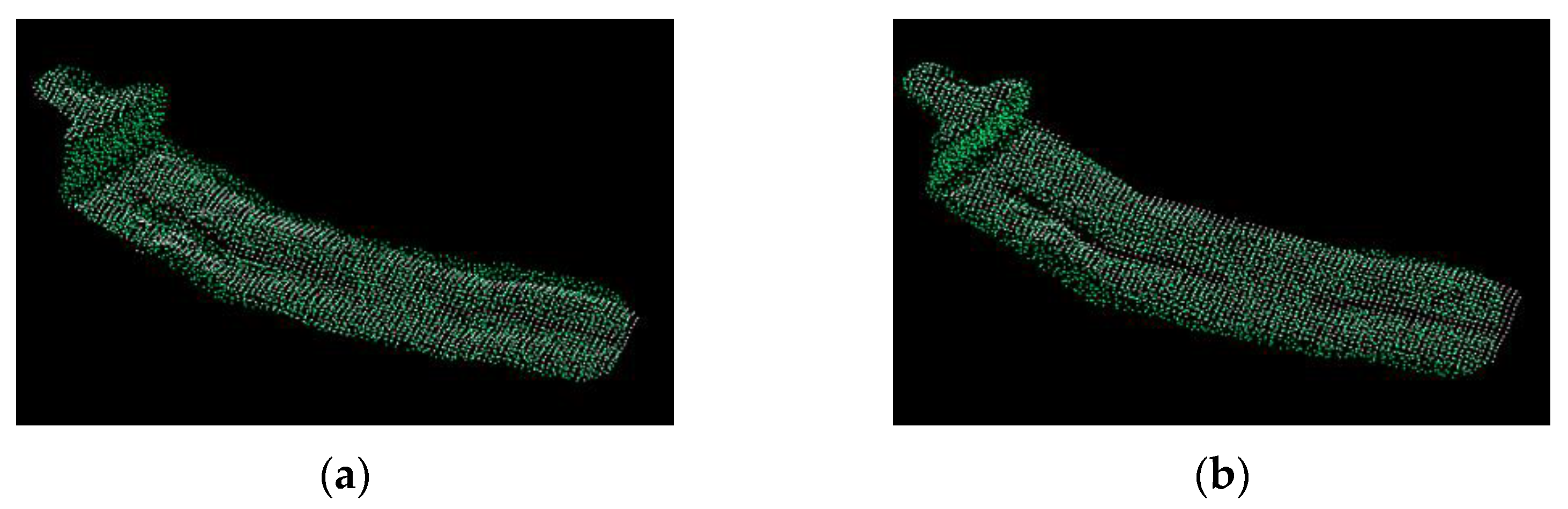
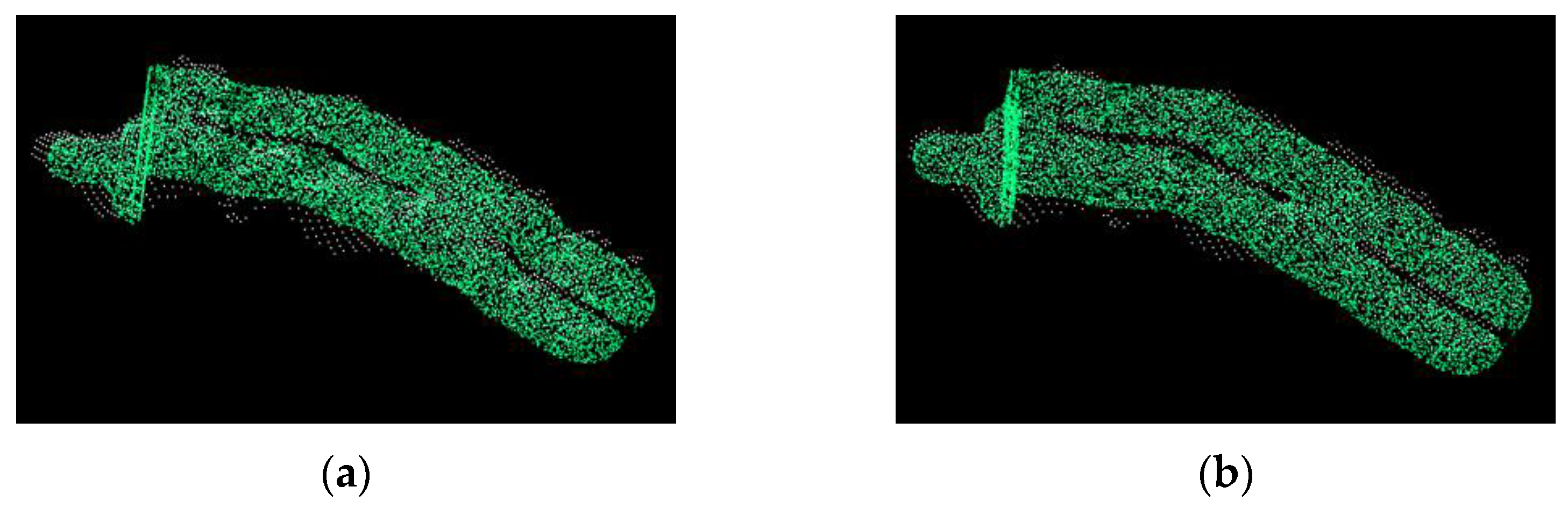
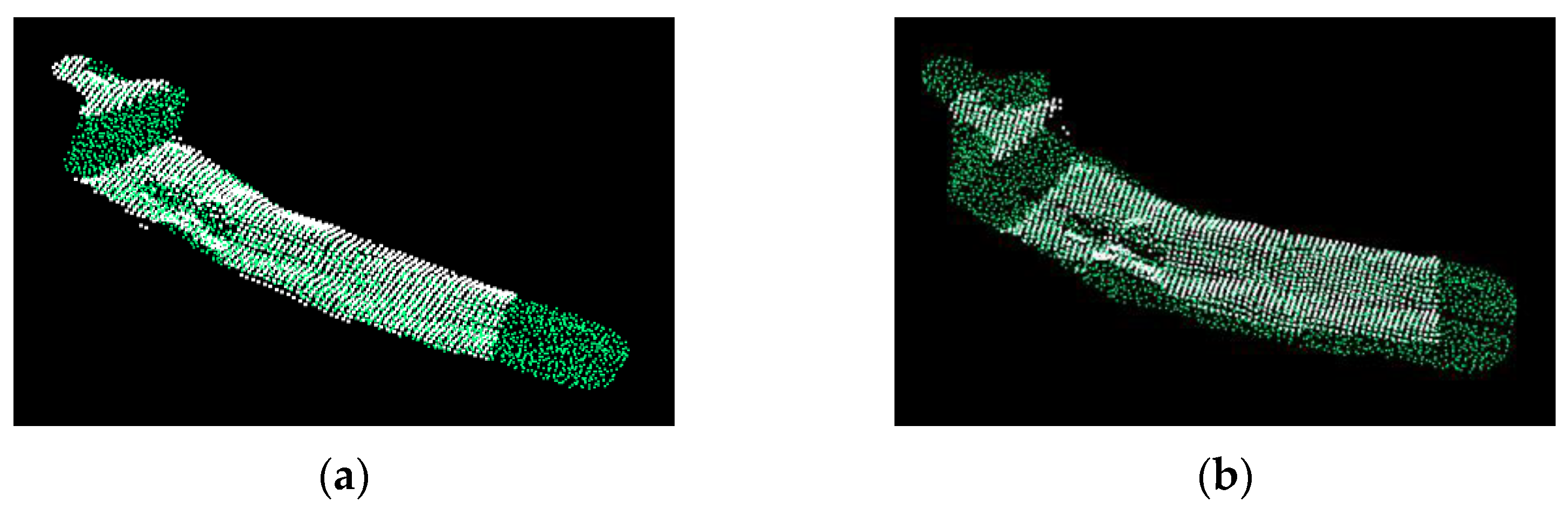
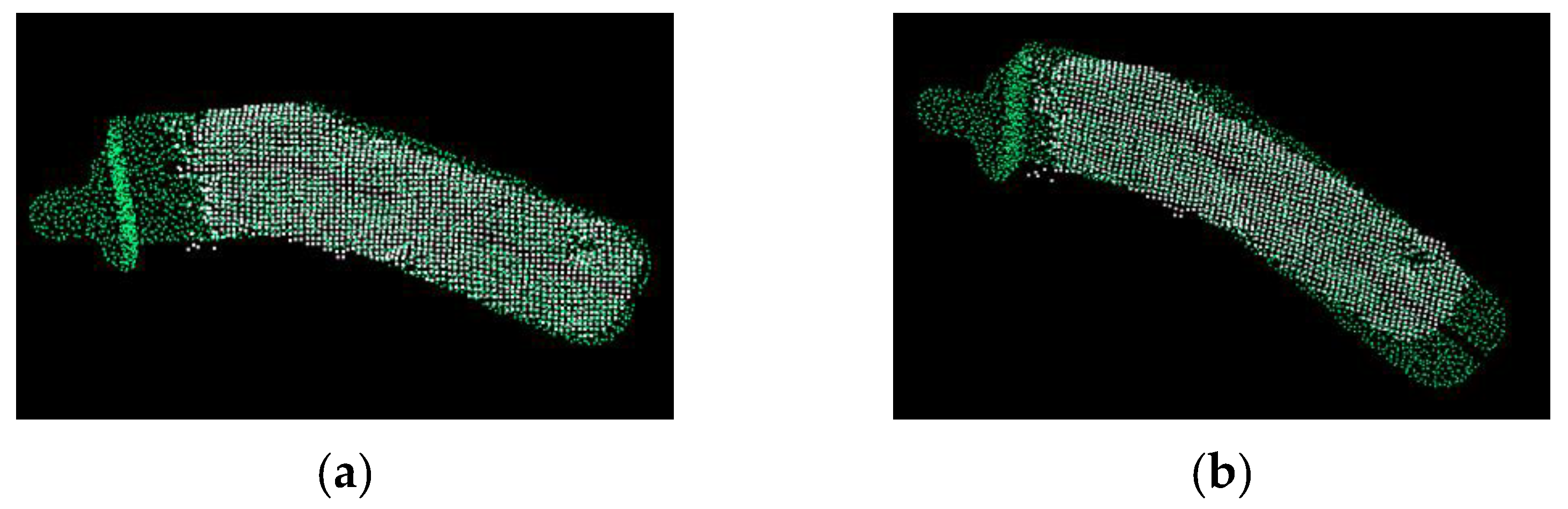
4.2. 3D Point Cloud Registration Experiment and Analysis

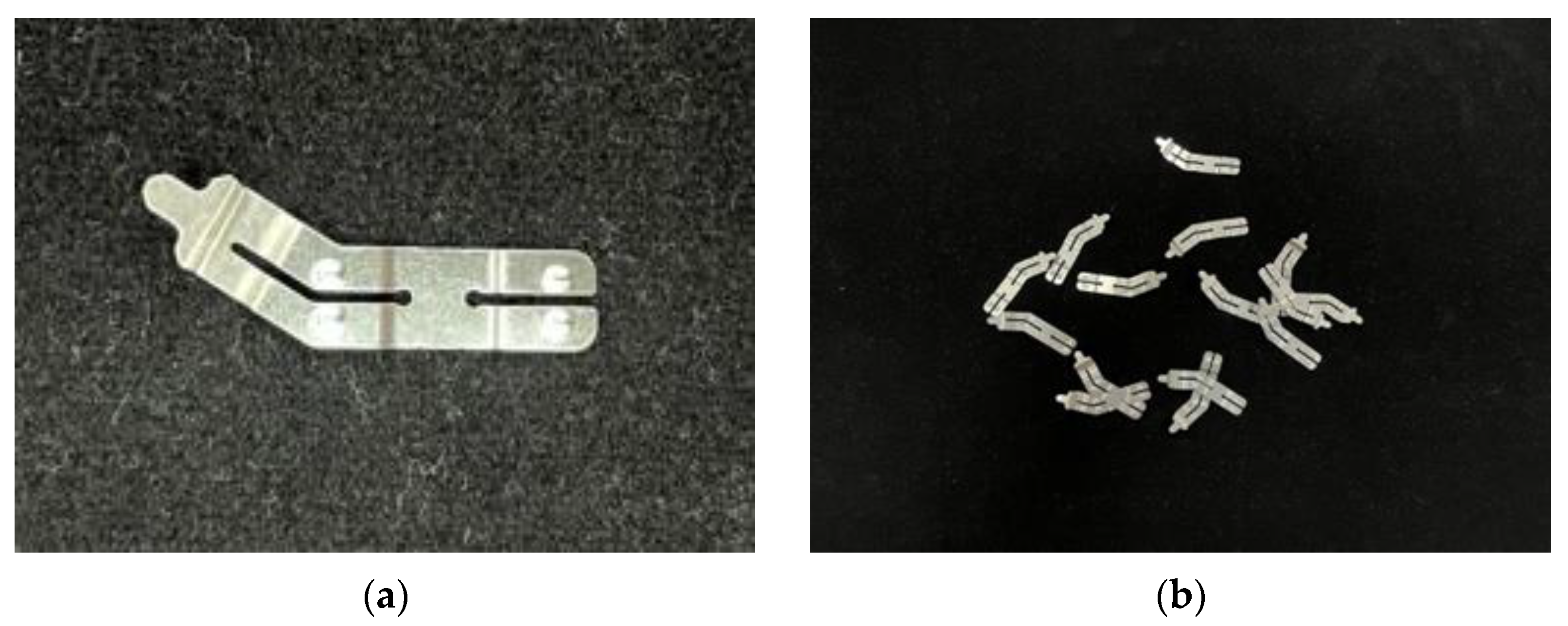
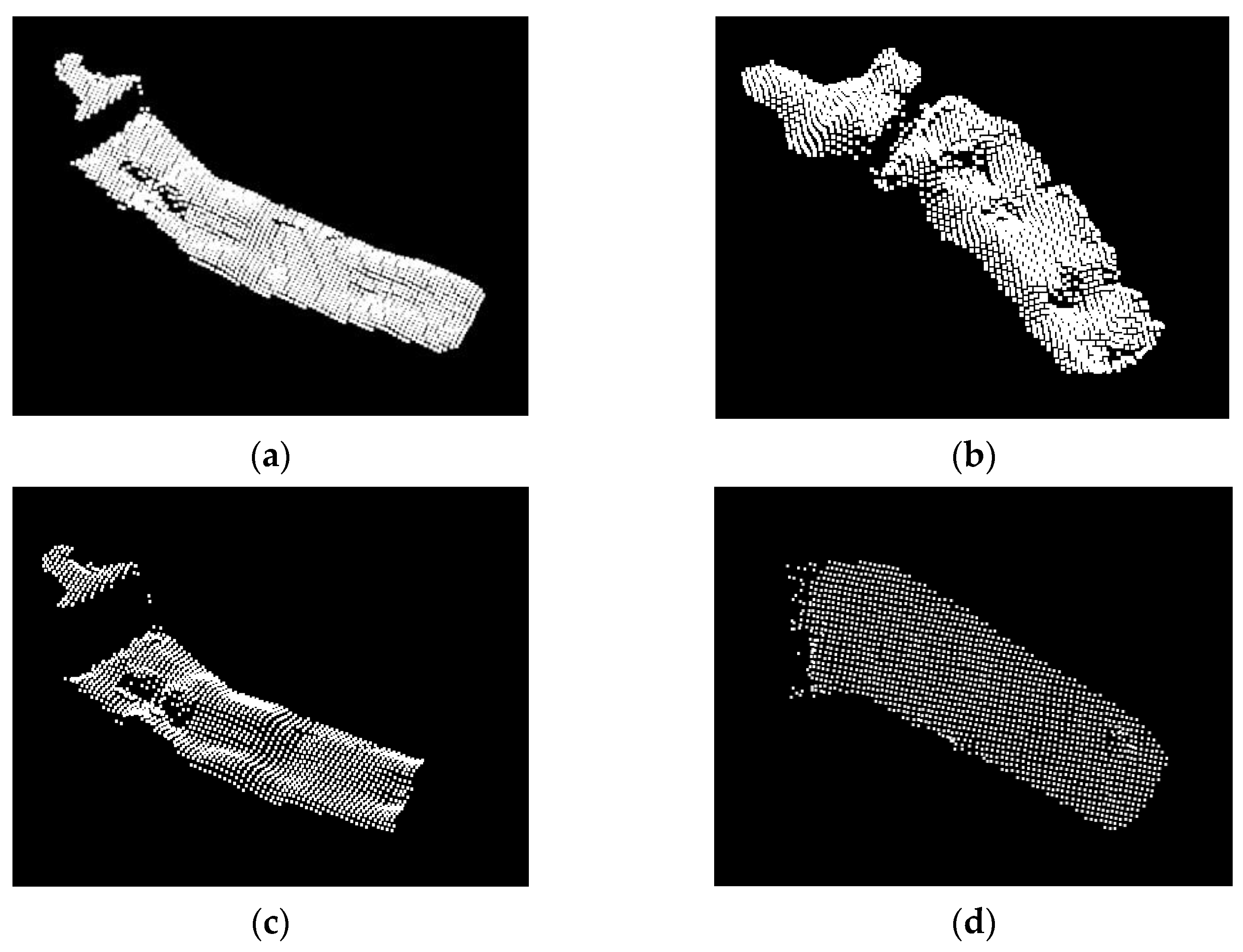
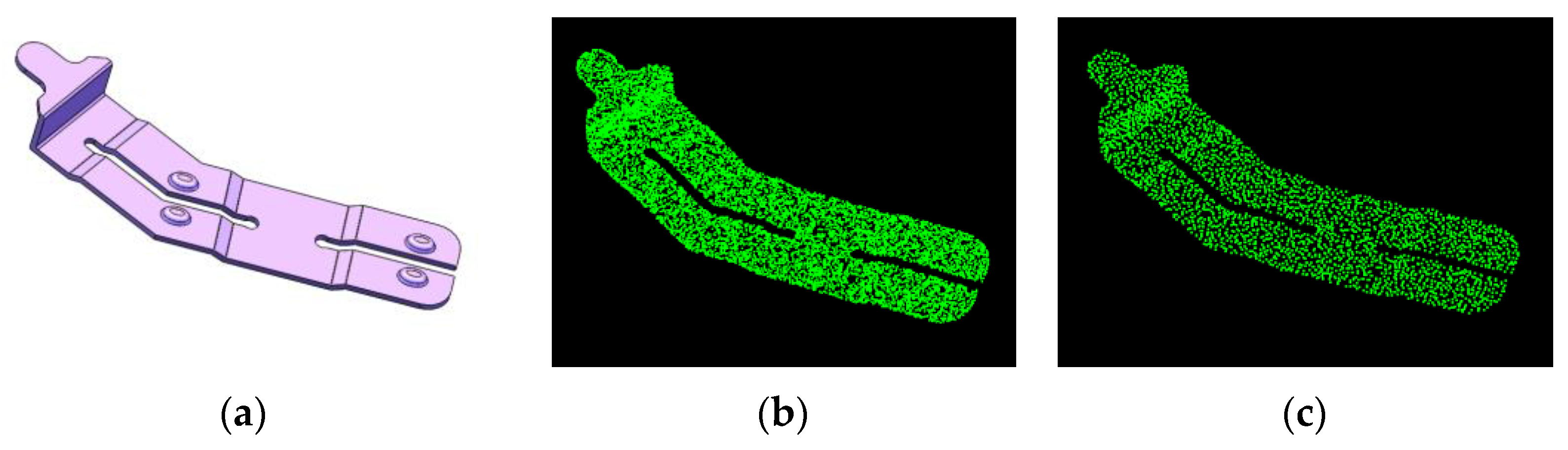
4.2.1. Generation of Target Point Cloud and Model Point Cloud of Nickel Sheets

First, we divided the nickel sheet distribution into four types, namely, the complete area with the front side facing up, the complete area with the back side facing up, the partly occluded area with the front side facing up, and the partly occluded area with the back side facing up. Then, we aligned the mask and depth map obtained based on the example segmentation to generate the target point cloud. The process of generating the target point cloud using the target mask is shown in Figure 14.

Specifically, after generating the nickel sheet mask using the above instance segmentation, we calculated the 3D coordinates of each pixel of the target mask image based on the formula for transforming the mask pixel point [C_x, C_y]^T to the 3D coordinate point [P_x, P_y, P_z]^T (see Formula (8) in Section 3.1) to obtain the target point cloud

Figure 15 shows the point clouds of four different poses generated by aligning the instance segmentation mask with the depth map. Figure 15a indicates the complete area with the front side facing up, Figure 15b exhibits the complete area with the back side facing up, Figure 15c demonstrates the partly occluded area with the front side facing up, and Figure 15d shows the partly occluded area with the back side facing up.

We used the SolidWorks software to export the 3D model of nickel sheets in STL format, then adopted the PCL software to open the STL file and convert it into point cloud format. Figure 16a shows the 3D model before conversion, and Figure 16b shows the point cloud format after conversion. There are 10,013 points in the point cloud. To improve the efficiency and accuracy of subsequent point cloud registration, we performed downsampling on the model point cloud and set the side length of the voxel grid to 0.3 mm. The number of points in the point cloud changed from 10,013 to 3213. The effect is shown in Figure 16c.

4.2.2. Registration Experiment of Target Point Cloud and Model Point Cloud

We integrated the SAC-IA coarse registration algorithm, NDT coarse registration algorithm, and ICP fine registration algorithm in Section 3.2 to perform registration experiments on the point clouds of the above four poses.

To facilitate a comparison, we first conducted the point cloud registration experiments based on the SAC-IA rough registration algorithm and NDT rough registration algorithm in Section 3.2. Figure 17 shows the results. In each figure, green denotes the model point cloud of the nickel sheet, while white denotes the target point cloud of the nickel sheet. It can be seen from the figure that though the registration effect is not ideal, the model point cloud is relatively close to the target point cloud.

Then, we carried out registration experiments of the point cloud using the combination of the SAC-IA coarse registration algorithm + ICP fine registration algorithm and NDT coarse registration algorithm + ICP fine registration algorithm, respectively. Figure 18a, Figure 19a, Figure 20a and Figure 21a show the registration results based on the SAC-IA algorithm + ICP algorithm. Figure 18b, Figure 19b, Figure 20b and Figure 21b show the registration results based on the NDT algorithm + ICP algorithm. In each figure, green denotes the model point cloud of the nickel sheet, while white denotes the target point cloud of the nickel sheet.

The results of the above registration experiments show that both combinations of registration methods can achieve good registration results for target point clouds (see Figure 18 and Figure 19). As for the point clouds with partly occluded areas, the registration results of the SAC-IA + ICP coarse/fine registration are better than those of the NDT + ICP coarse/fine registration (see Figure 20 and Figure 21).

Table 4. Time spent on point cloud registration based on SAC-IA + ICP.

Pose	Front Side Faces Up	Back Side Faces Up	Occluded Front Side Faces Up	Occluded Back Side Faces Up
Time (ms)	524.00	593.00	455.00	471.00
Average registration time (ms)	510.75

shows the time spent on registering the four different point cloud poses based on SAC-IA + ICP.

Table 5. Time spent on point cloud registration based on NDT + ICP.

Pose	Front Side Faces Up	Back Side Faces Up	Occluded Front Side Faces Up	Occluded Back Side Faces Up
Time (ms)	548.00	618.00	486.00	494.00
Average registration time (ms)	531.50

shows the time spent on registering the four different point cloud poses based on DNT + ICP.

It can be seen from Table 4 and Table 5 that the registration algorithm based on the SAC-IA + ICP combination consumes less time on average than that of the NDT + ICP combination. Moreover, the registration algorithm based on the SAC-IA + ICP combination has a better registration effect. Therefore, it is reasonable to select the registration algorithm based on the SAC-IA + ICP combination for the pose estimation of the nickel sheet.

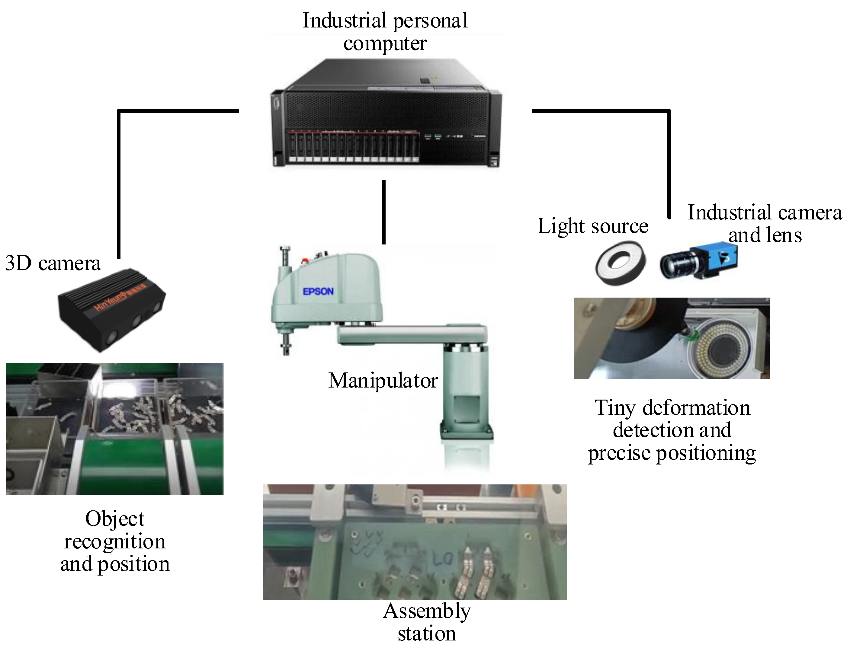
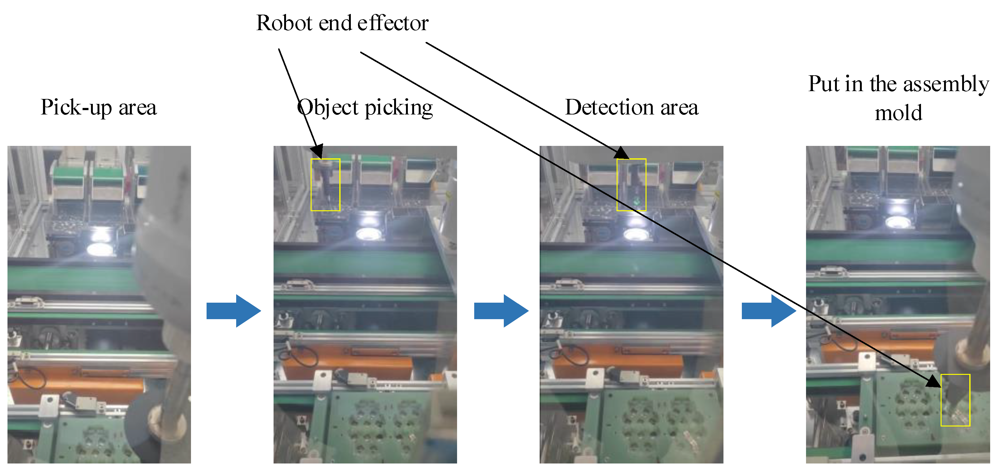
4.3. Practical Application Test

To verify the practical application effect of the algorithm proposed in this paper, we conducted application tests for the assembly of nickel sheets in a famous new energy battery automated production line. The intelligent hardware system for picking up sheet metals comprises a selective compliance assembly robot arm manipulator, 3D camera, industrial personal camera, industrial computer, silo, and automatic transmission line (see Figure 22). The 3D camera used in this paper adopts a high-speed high-definition HY-M5-series 3D camera independently developed by Xianyang Technology, with a scanning speed of 10 Hz~300 Hz and a measurement accuracy range of 0.01 mm~1 mm. The industrial personal camera used was the DMK 23G274 made by Yingmei Precision, and the CCD area scanning camera had a resolution of 1.92 million. The lens model for the industrial camera was the TCL 3520 5MP.

According to the actual production model, we first employed the 3D vision system to obtain the RGB image and depth map of the target object in the area for picking up nickel sheets and calculated the pose information of the target in the pick-up area through the point cloud registration. Then we sent the pose information to the manipulator to accurately pick up the target nickel sheet. Finally, we moved the target nickel sheet to the inspection area for tiny deformation detection and placed the nickel sheet that met the parameter requirements in the corresponding position of the assembly mold. According to the strategy for picking up nickel sheets, the manipulator first picked up the unoccluded sheets. After that, the original occluded sheets became the new targets to be picked up. Figure 23 shows the intelligent hardware system for picking up sheet metals. Figure 24 shows the recognition, positioning, and identification of nickel sheets.

The intelligent system for picking up nickel sheets realizes the functions of automatic recognition and positioning, robotic picking, tiny deformation detection, and fixed-point assembly of sheet metal for new energy batteries. The detection accuracy of tiny deformation defects in the sheets was 0.1 mm, the detection error was within 0.05 mm, the execution time of the whole process was within 3 s, and the assembly accuracy was less than 0.1 mm. The precision, speed, and stability of the system met production requirements.

5. Conclusions

This study aimed to enhance the detection accuracy and reduce the computation time for acquiring the pose of small sheets of metal with multi-objective overlapping in cross-scale robot assembly. Our approach involved utilizing instance segmentation and a 3D point cloud for the pose recognition model. By employing instance segmentation, we generated a target mask and aligned it with the model point cloud to obtain 3D pose information.

To handle single special-shaped sheet metal, we aligned the target mask and depth map to create a target point cloud. We developed a feature extraction network, a feature map candidate region generation network, and an object recognition and classification network for the instance segmentation model. Additionally, we established an instance segmentation model for special-shaped sheet metal with multi-objective overlapping, allowing segmentation under various circumstances. We successfully extracted the target mask and aligned it with the depth map to generate the target point cloud. Moreover, we explored the pose estimation by integrating the SAC-IA coarse registration algorithm with the ICP fine registration algorithm, yielding improved registration results.

Furthermore, we curated custom datasets for pose recognition and the localization of special-shaped nickel sheets commonly used in new energy battery assembly. We labeled 4091 objects in 1052 images. The experimental tests demonstrated the effectiveness of our approach, including achieving an mAP greater than 97% for the instance segmentation models, reducing the time consumption by more than 50% compared to the baseline, and obtaining improved registration results with the SAC-IA + ICP combination. The proposed method was validated through testing in a robotic assembly system for nickel sheets, meeting the production requirements of new energy battery manufacturing.

While our study yielded positive results in identifying and positioning small-sized thin special-shaped metal parts, there are still some limitations. Despite reaching an accuracy of over 90% in the instance segmentation algorithm, false recognition and missing recognition still occurred due to insufficient training data samples and a suboptimal model structure. Although these misidentified parts can be addressed in the micro defect detection stage, it affects the overall efficiency. Our future work will involve refining the network structure and constructing an improved instance segmentation model within the framework of deep learning.

References

1. Zheng, T.X.; Jiang, M.Z.; Feng, M.C. Vision-based target recognition and location for picking robot: A review. Chin. J. Sci. Instrum. 2021, 42, 28–51. [Google Scholar]
2. He, K.; Gkioxari, G.; Dollár, P.; Girshick, R. Mask R-CNN. In IEEE Transactions on Pattern Analysis & Machine Intelligence; IEEE: New York, NY, USA, 2017. [Google Scholar]
3. Li, Y.; Qi, H.; Dai, J.; Ji, X.; Wei, Y. Fully convolutional instance-aware semantic segmentation. In Proceedings of the IEEE Conference on Computer Vision and Pattern Recognition, Honolulu, HI, USA, 21–26 July 2017; pp. 2359–2367. [Google Scholar]
4. Sun, Y.; Su, L.; Luo, Y.; Meng, H.; Li, W.; Zhang, Z.; Wang, P.; Zhang, W. Global Mask R-CNN for marine ship instance segmentation. Neurocomputing 2022, 480, 257–270. [Google Scholar] [CrossRef]
5. Yang, H.; Zheng, L.; Barzegar, S.G.; Zhang, Y.; Xu, B. BorderPointsMask: One-stage instance segmentation with boundary points representation. Neurocomputing 2022, 467, 348–359. [Google Scholar] [CrossRef]
6. Xu, Y.; Arai, S.; Liu, D.; Lin, F.; Kosuge, K. FPCC: Fast point cloud clustering-based instance segmentation for industrial bin-picking. Neurocomputing 2022, 494, 255–268. [Google Scholar] [CrossRef]
7. Bolya, D.; Zhou, C.; Xiao, F.; Lee, Y.J. Yolact: Real-time instance segmentation. In Proceedings of the IEEE/CVF International Conference on Computer Vision, Seoul, Republic of Korea, 27 October–2 November 2019; pp. 9157–9166. [Google Scholar]
8. Chen, X.; Girshick, R.; He, K.; Dollar, P. Tensormask: A foundation for dense object segmentation. In Proceedings of the IEEE/CVF International Conference on Computer Vision, Seoul, Republic of Korea, 27 October–2 November 2019; pp. 2061–2069. [Google Scholar]
9. Yang, Z.; Dong, R.; Xu, H.; Gu, J. Instance Segmentation Method Based on Improved Mask R-CNN for the Stacked Electronic Components. Electronics 2020, 9, 886. [Google Scholar] [CrossRef]
10. Wang, X.; Kong, T.; Shen, C.; Jiang, Y.; Li, L. Solo: Segmenting objects by locations. In European Conference on Computer Vision; Springer: Cham, Switzerland, 2020; pp. 649–665. [Google Scholar]
11. Hua, J.; Hao, T.; Zeng, L.; Yu, G. YOLO Mask, an Instance Segmentation Algorithm Based on Complementary Fusion Network. Mathematics 2021, 9, 1766. [Google Scholar] [CrossRef]
12. Song, S.; Xiao, J. Sliding shapes for 3d object detection in depth images. In European Conference on Computer Vision; Springer: Cham, Switzerland, 2014; pp. 634–651. [Google Scholar]
13. Qi, C.R.; Su, H.; Mo, K.; Guibas, L.J. Pointnet: Deep learning on point sets for 3d classification and segmentation. In Proceedings of the IEEE Conference on Computer Vision and Pattern Recognition, Honolulu, HI, USA, 21–26 July 2017; pp. 652–660. [Google Scholar]
14. Qi, C.R.; Yi, L.; Su, H.; Guibas, L.J. PointNet++: Deep Hierarchical Feature Learning on Point Sets in a Metric Space. In Proceedings of the 31st Conference on Neural Information Processing Systems (NIPS 2017), Long Beach, CA, USA, 4–9 December 2017. [Google Scholar]
15. Yi, L.; Zhao, W.; Wang, H.; Sung, M.; Guibas, L.J. Gspn: Generative shape proposal network for 3d instance segmentation in point cloud. In Proceedings of the IEEE/CVF Conference on Computer Vision and Pattern Recognition, Long Beach, CA, USA, 15–20 June 2019; pp. 3947–3956. [Google Scholar]
16. Chen, H.; Li, L.; Chen, P.; Meng, R. 6D Pose Estimation Network in Complex Point Cloud Scenes. J. Electron. Inf. Technol. 2022, 44, 1591–1601. (In Chinese) [Google Scholar]
17. Gao, N.; Shan, Y.; Zhao, X.; Huang, K. Learning category-and instance-aware pixel embedding for fast panoptic segmentation. In IEEE Transactions on Image Processing; IEEE: New York, NY, USA, 2021; pp. 6013–6023. [Google Scholar]
18. He, K.; Zhang, X.; Ren, S.; Sun, R. Deep residual learning for image recognition. In Proceedings of the IEEE Conference on Computer Vision and Pattern Recognition, Las Vegas, NV, USA, 27–30 June 2016; pp. 770–778. [Google Scholar]
19. Lin, T.Y.; Dollár, P.; Girshick, R.; He, K.; Hariharan, B.; Belongie, S. Feature pyramid networks for object detection. In Proceedings of the IEEE Conference on Computer Vision and Pattern Recognition, Honolulu, HI, USA, 21–26 July 2017; pp. 2117–2125. [Google Scholar]
20. Chu, J.; Zhang, Y.; Li, S.; Leng, L.; Miao, J. Syncretic-NMS: A merging non-maximum suppression algorithm for instance segmentation. IEEE Access 2020, 8, 114705–114714. [Google Scholar] [CrossRef]
21. Lee, H.; Lee, J.S.; Choi, H.C. Parallelization of Non-Maximum Suppression. IEEE Access 2021, 9, 166579–166587. [Google Scholar] [CrossRef]
22. Li, M.; Chen, D.; Liu, S.; Liu, F. Prior mask R-CNN based on graph cuts loss and size input for precipitation measurement. IEEE Trans. Instrum. Meas. 2021, 70, 1–15. [Google Scholar] [CrossRef]
23. Liu, C.; Yu, S.; Yu, M.; Wei, B.; Li, B.; Li, G.; Huang, W. Adaptive smooth l1 loss: A better way to regress scene texts with extreme aspect ratios. In Proceedings of the 2021 IEEE Symposium on Computers and Communications (ISCC), Athens, Greece, 5–8 September 2021; pp. 1–7. [Google Scholar]
24. Xu, Y.; Jung, C.; Chang, Y. Head pose estimation using deep neural networks and 3D point clouds. Pattern Recognit. 2022, 121, 108210. [Google Scholar] [CrossRef]
25. Song, W.; Jiang, W.; Lou, Z. Rapid batch three-dimensional reconstruction of point clouds based on multi-label classification. Laser Optoelectron. Prog. 2021, 58, 75–85. (In Chinese) [Google Scholar]
26. Guo, N.; Zhang, B.; Zhou, J.; Zhan, K.; Lai, S. Pose estimation and adaptable grasp configuration with point cloud registration and geometry understanding for fruit grasp planning. Comput. Electron. Agric. 2020, 179, 105818. [Google Scholar] [CrossRef]
27. Chen, F.; Chen, W.; Qin, F. A pose estimation method for disordered sorting. Autom. Appl. 2021, 12, 147–150. [Google Scholar]
28. Wang, P.; Xu, G.; Cheng, Y.; Yu, Q. A simple, robust and fast method for the perspective-n-point Problem. Pattern Recognit. Lett. 2018, 108, 31–37. [Google Scholar] [CrossRef]
29. Wu, H.; Xu, Z.; Liu, C.; Akbar, A.; Yue, H.; Zeng, D.; Yang, H. LV-GCNN: A lossless voxelization integrated graph convolutional neural network for surface reconstruction from point clouds. Int. J. Appl. Earth Obs. Geoinf. 2021, 103, 102504. [Google Scholar] [CrossRef]
30. Zhang, P.; Zhang, C.; Liu, B.; Wu, Y. Leveraging local and global descriptors in parallel to search correspondences for visual localization. Pattern Recognit. 2022, 122, 108344. [Google Scholar] [CrossRef]
31. Zhong, L.; Ying, J.; Yang, H.; Jin, L. Triple screening point cloud registration method based on image and geometric features. Optik 2021, 246, 167763. [Google Scholar] [CrossRef]
32. Iqbal, M.Z.; Bobkov, D.; Steinbach, E. Fuzzy logic and histogram of normal orientation-based 3D keypoint detection for point clouds. Pattern Recognit. Lett. 2020, 136, 40–47. [Google Scholar] [CrossRef]
33. Zhang, Z.; Dai, Y.; Sun, J. Deep learning based point cloud registration: An overview. Virtual Real. Intell. Hardw. 2020, 2, 222–246. [Google Scholar] [CrossRef]
34. Li, J.; Hu, Q.; Zhang, Y.; Ai, M. Robust symmetric iterative closest point. ISPRS J. Photogramm. Remote Sens. 2022, 185, 219–231. [Google Scholar] [CrossRef]
35. Sun, C. Technology and Application of Small-Defect Vision Detection and Recognition under Multi-Objective; Guangdong University of Technology: Guangzhou, China, 2022. [Google Scholar]
Figure 1. Instance segmentation model framework for generating object masks.
Electronics 12 02613 g001
Figure 2. Network structure diagram of feature extraction.
Electronics 12 02613 g002
Figure 3. RPN structure diagram.
Electronics 12 02613 g003
Figure 4. Object recognition and classification network structure.
Electronics 12 02613 g004
Figure 5. Mask branch network structure.
Electronics 12 02613 g005
Figure 6. Schematic diagram of pose estimation of sheet metal.
Electronics 12 02613 g006
Figure 7. Local coordinate system constructed with p .
Electronics 12 02613 g007
Figure 8. Appearance of nickel sheets. (a) Single nickel sheet; (b) Overlapping nickel sheets.
Electronics 12 02613 g008
Figure 9. Overall architecture of the spatial pose recognition experiment on nickel sheets.
Electronics 12 02613 g009
Figure 10. Data enhancement renderings. (a) Flip; (b) Rotation; (c) Translation; and (d) Mirroring.
Electronics 12 02613 g010
Figure 11. Schematic diagram of nickel sheet labels.
Electronics 12 02613 g011
Figure 12. Schematic diagram of the front and back of the nickel sheet. (a) Front of the nickel sheet; (b) Back of the nickel sheet.
Electronics 12 02613 g012
Figure 13. Figure 13. Image test results. (a) Status 1, (b) Status 2, (c) Status 3, and (d) Status 4.
Electronics 12 02613 g013
Figure 14. Generating target point cloud using target mask.
Electronics 12 02613 g014
Figure 15. Effect diagram of target point cloud with different poses. (a) Face up 1, (b) Reverse side up 1, (c) Face up 2, and (d) Reverse side up 2.
Electronics 12 02613 g015
Figure 16. Effect diagram of point cloud generation of nickel sheet model. (a) Three-dimensional model; (b) Point cloud format; (c) Design sketch.
Electronics 12 02613 g016
Figure 17. Coarse registration results. (a) SAC-IA coarse registration; (b) NDT coarse registration.
Electronics 12 02613 g017
Figure 18. Comparison of registration results with the front side facing up. (a) SAC-IA + ICP, (b) NDT + ICP.
Electronics 12 02613 g018
Figure 19. Comparison of registration results with the back side facing up. (a) SAC-IA + ICP, (b) NDT + ICP.
Electronics 12 02613 g019
Figure 20. Comparison of registration results with the partially occluded front side facing up. (a) SAC-IA + ICP, (b) NDT + ICP.
Electronics 12 02613 g020
Figure 21. Comparison of registration results with the partially occluded back side facing up. (a) SAC-IA + ICP, (b) NDT + ICP.
Electronics 12 02613 g021
Figure 22. Intelligent hardware system for picking up sheet metals.
Electronics 12 02613 g022
Figure 23. Schematic diagram of the intelligent pick-up process of nickel sheets.
Electronics 12 02613 g023
Figure 24. Recognition and positioning results of sheet metals. (a) Recognition results; (b) Positioning results.
Electronics 12 02613 g024