A Novel 3-D Jerk System, Its Bifurcation Analysis, Electronic Circuit Design and a Cryptographic Application

Abstract

This paper introduces a new chaotic jerk system with three cubic nonlinear terms. The stability properties of the three equilibrium points of the proposed jerk system are analyzed in detail. We show that the three equilibrium points of the new chaotic jerk system are unstable and deduce that the jerk system exhibits self-excited chaotic attractors. The bifurcation structures of the proposed jerk system are investigated numerically, showing period-doubling, periodic windows and coexisting bifurcations. An electronic circuit design of the proposed jerk system is designed using PSPICE. As an engineering application, a new image-encryption approach based on the new chaotic jerk system is presented in this research work. Experimental results demonstrate that the suggested encryption mechanism is effective with high plain-image sensitivity and the reliability of the proposed chaotic jerk system for various cryptographic purposes.

1. Introduction

Chaotic systems find a wide range of engineering applications such as memristors [1,2,3,4], laser systems [5,6,7], electrical circuits [8,9,10], neural networks [11,12], encryption [13,14,15], memristors [16], neuron models [17], etc. As a particular case, a third-order autonomous jerk differential equation has the general form

$$\stackrel{⃛}{ϵ}=F(ϵ,\dot{ϵ},\ddot{ϵ})$$

(1)

Using the state variables $z_1=ϵ$, $z_2=\dot{ϵ}$, $z_3=\ddot{ϵ}$, one can rewrite the jerk Equation (1) in system form as follows:

$$\begin{array}{ccc}{\dot{z}}_1& =& z_2\hfill \\ {\dot{z}}_2& =& z_3\hfill \\ {\dot{z}}_3& =& F(z_1,z_2,z_3)\hfill \end{array}$$

(2)

Jerk systems with chaotic attractors have several applications such as circuits [18,19,20], memristors [21], encryption [22,23], etc.

There is significant interest regarding chaotic jerk systems in the literature [24,25,26,27,28]. Sprott [24] proposed a simple chaotic jerk system with one quadratic nonlinearity. Sun and Sprott [25] reported a chaotic jerk system with a piecewise exponential nonlinearity. Liu et al. [26] discussed a new chaotic jerk system having two quadratic nonlinearities. Vaidyanathan et al. [27] proposed a new chaotic jerk system having two exponential nonlinearities and presented its electronic circuit simulation. Rajagopal et al. [28] presented a chaotic jerk system with two quadratic nonlinearities, discussed its dynamic properties and gave a circuit realization of the jerk system.

In this paper, we describe a new chaotic jerk system with three cubic nonlinear terms. We show that there are three unstable equilibrium points for the proposed jerk system. The bifurcation structures of the proposed jerk system are investigated numerically, showing period-doubling, periodic windows and coexisting bifurcations.

An electronic circuit design of the proposed jerk system is designed using PSpice. Although PSpice is a useful tool, it has many limitations [27]. Real electronic components can be complex creatures with many behaviors. Simulation of a circuit is only as accurate as the behaviors modeled in the PSpice devices created for it. Many circuit simulations are based on simplified models [27].

Finally, a new image-encryption approach is presented based on the chaotic behavior of the proposed jerk system. Circuit designs of chaotic systems are useful for their practical implementations [8,18].

The security and privacy of digital information play an important role in the digital era, in which images are a common data type for representing and transferring data [29].

Digital images can be secured by applying a reliable image-encryption mechanism. Because of their high sensitivity to primary conditions and their chaotic demeanor, chaotic systems are commonly utilized for developing image cryptosystems [30,31].

In this paper, a new image-encryption approach based on the chaotic behavior of the new jerk system is proposed. The proposed encryption approach consists of two rounds of encryption, in which the substitution phase is performed in the first round, and some information about the substituted image is gained using the SHA-256 algorithm for modernizing the prime conditions of the jerk system. The second round of encryption consists of one permutation phase and one substitution phase. Experimental results demonstrate that the suggested encryption mechanism is effective with high plain-image sensitivity and the reliability of the proposed chaotic jerk system for various cryptographic purposes.

2. A New Jerk System

In this paper, we propose a new 3-D jerk differential equation given by

$$\stackrel{⃛}{z}+a\ddot{z}+z(z^2+z\dot{z}+{\dot{z}}^2-b)=0$$

(3)

where z has the physical interpretation of displacement, $\dot{z}$ the velocity, $\ddot{z}$, the acceleration and $\stackrel{⃛}{z}$ the jerk. Here, a and b are taken as positive constants.

Using the phase variables $z_1=z$, $z_2=\dot{z}$ and $z_3=\ddot{z}$, it is possible to represent the jerk ODE (3) as a system of first-order differential equations:

$$\left\{\begin{array}{ccc}{\dot{z}}_1& =& z_2\hfill \\ {\dot{z}}_2& =& z_3\hfill \\ {\dot{z}}_3& =& -a{z}_3-z_1\left(z_1^2+z_1{z}_2+z_2^2-b\right)\hfill \end{array}\right.$$

(4)

In this work, we shall show that the jerk system (4) has a chaotic attractor for $(a,b)=(1.2,2.5)$. This is verified by calculating the local Lyapunov exponent values for $(a,b)=(1.2,2.5)$ and $Z\left(0\right)=(0.3,0.2,0.3)$ with simulation time $T=1\times {10}^5$ seconds as follows:

$${\tau }_1=0.0941,{\tau }_2=0,{\tau }_3=-1.2941$$

(5)

Figure 1 shows the calculation of the local Lyapunov exponent (LE) values for the jerk system (4).

Since the largest Lyapunov exponent (LLE) is positive (${\tau }_1>0$), we conclude that the jerk system (4) is chaotic. Moreover, the jerk system (4) is dissipative since

$${\tau }_1+{\tau }_2+{\tau }_3=-a<0.$$

(6)

Thus, the jerk system (4) has a chaotic attractor.

We note that the jerk system (4) stays invariant under the coordinates transformation

$$(z_1,z_2,z_3)\mapsto (-z_1,-z_2,-z_3)$$

(7)

This shows that the jerk system (4) has a point reflection symmetry about the origin.

Figure 2 portrays the MATLAB simulations of the jerk system (4) for $Z\left(0\right)=(0.3,0.2,0.3)$ and $(a,b)=(1.2,2.5)$.

The rest points of the jerk system (4) are found by solving the following equations.

$$\begin{array}{}\hfill z_2& =& 0& \mathrm{(8a)}\hfill z_3& =& 0& \mathrm{(8b)}\hfill -a{z}_3-z_1\left(z_1^2+z_1{z}_2+z_2^2-b\right)& =& 0& \mathrm{(8c)}\end{array}$$

Using the values $z_2=0$ and $z_3=0$ from (8a) and (8b), respectively, we can simplify (8c) as follows:

$$-z_1\left(z_1^2-b\right)=0$$

(9)

Since $b>0$, there are three rest points for the jerk system (4) given by

$$\left\{\begin{array}{ccc}{Z}_0& =& (0,0,0),\hfill \\ Z_1& =& (\sqrt{b},0,0),\hfill \\ Z_2& =& (-\sqrt{b},0,0).\hfill \end{array}\right.$$

(10)

For the chaotic case, when $(a,b)=(1.2,2.5)$, the rest points are determined as follows:

$$\left\{\begin{array}{ccc}{Z}_0& =& (0,0,0),\hfill \\ Z_1& =& (1.5811,0,0),\hfill \\ Z_2& =& (-1.5811,0,0).\hfill \end{array}\right.$$

(11)

If we represent the jerk system (4) as $\dot{Z}=F\left(Z\right)$, then the Jacobian matrices of the vector field F at the three rest points $Z_0$, $Z_1$ and $Z_2$ can be easily calculated and denoted as $J_0$, $J_1$ and $J_2$, respectively.

The eigenvalues of $J_0$ are numerically evaluated as

$${\lambda }_1=-0.2463,{\lambda }_{2,3}=0.1231\pm 2.0113i.$$

(12)

The eigenvalues of $J_1$ are numerically estimated as

$${\lambda }_1=0.5961,{\lambda }_{2,3}=-0.2980\pm 1.0730i.$$

(13)

The eigenvalues of $J_2$ are the same as those of $J_1$.

Hence, we conclude that the jerk system (4) has three unstable, saddle-foci rest points at $Z_0,Z_1$ and $Z_2$. Hence, the new chaotic jerk system (4) has a self-excited chaotic attractor [32].

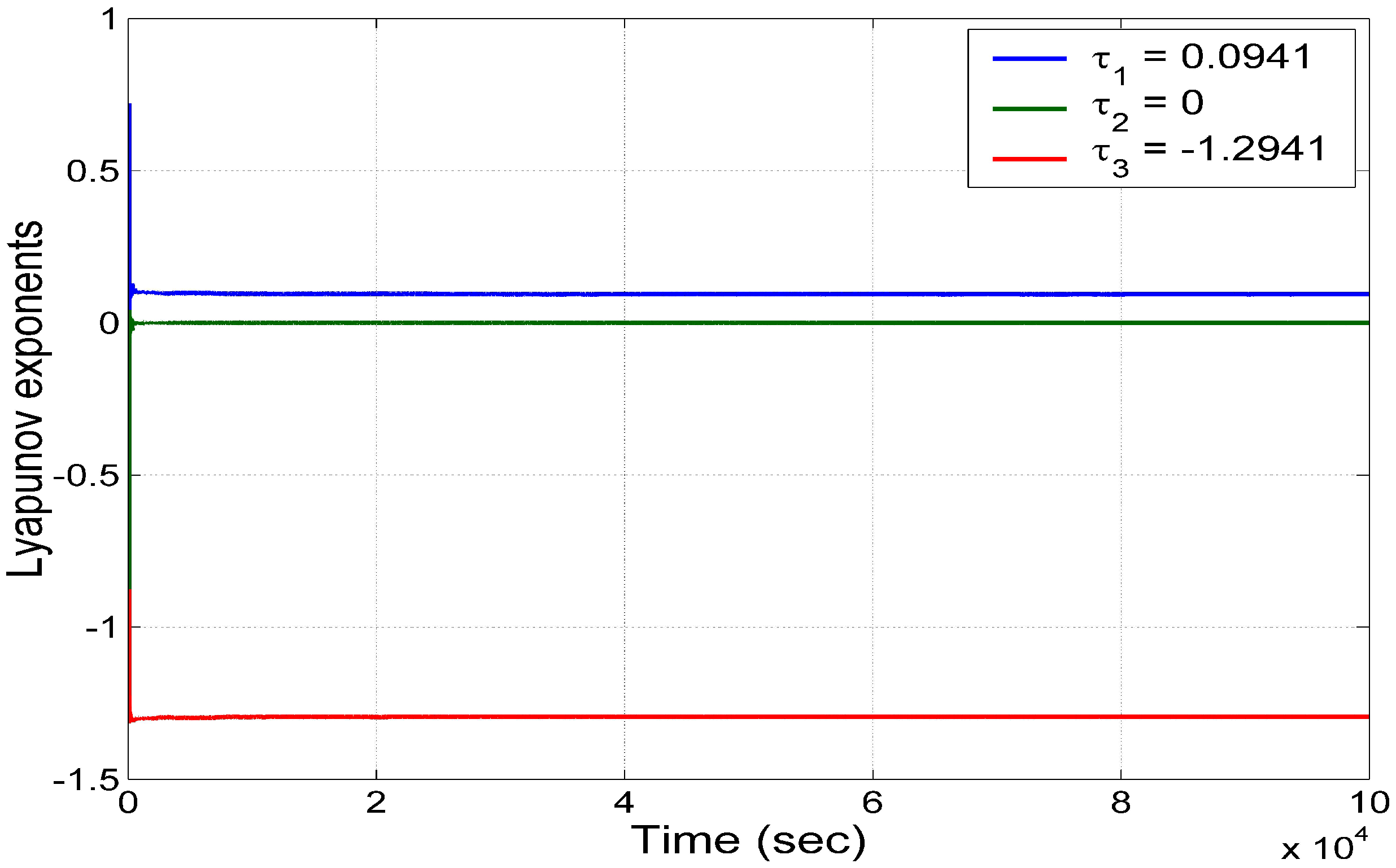
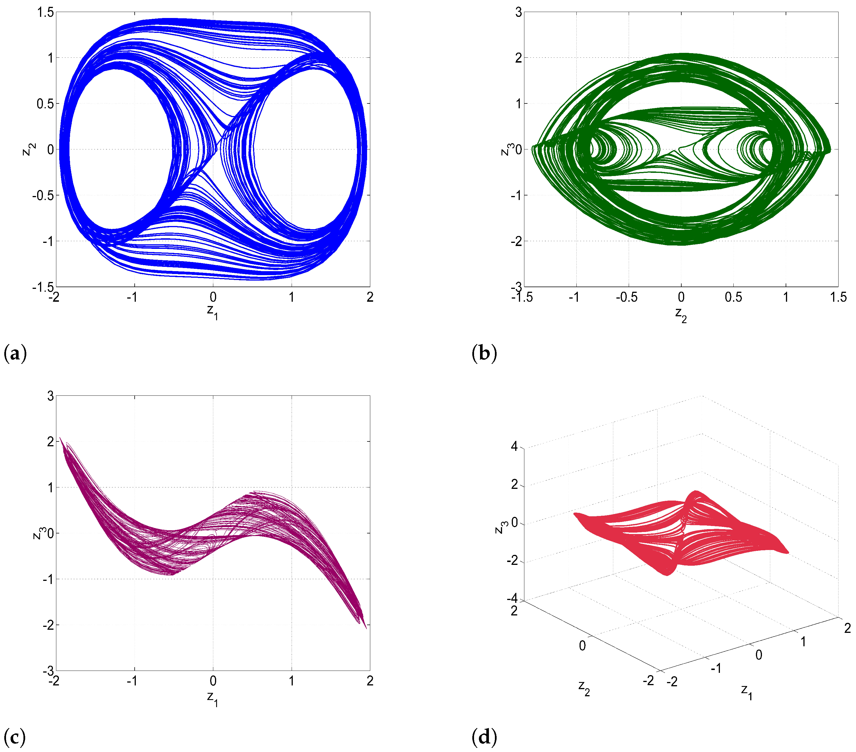
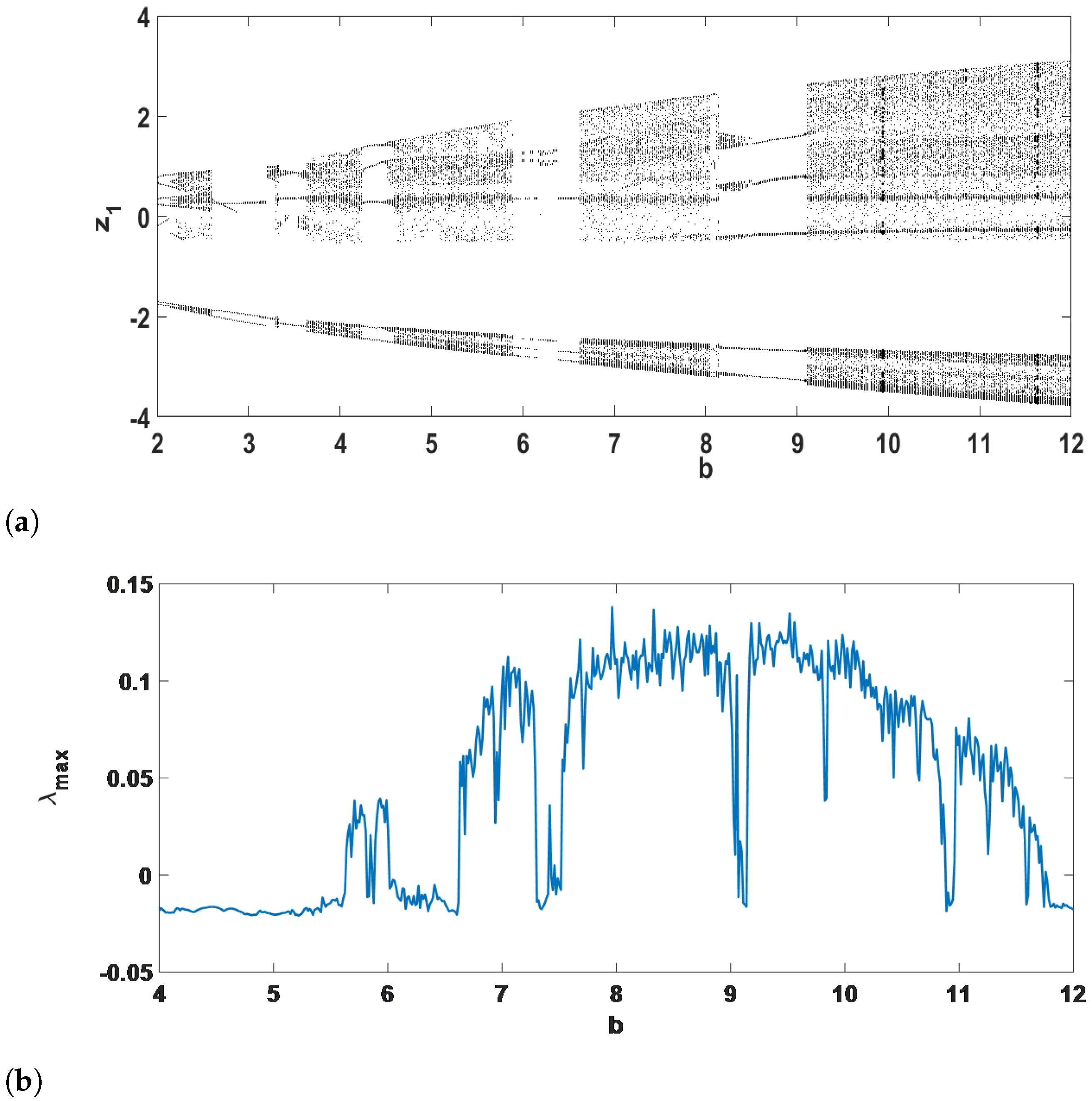
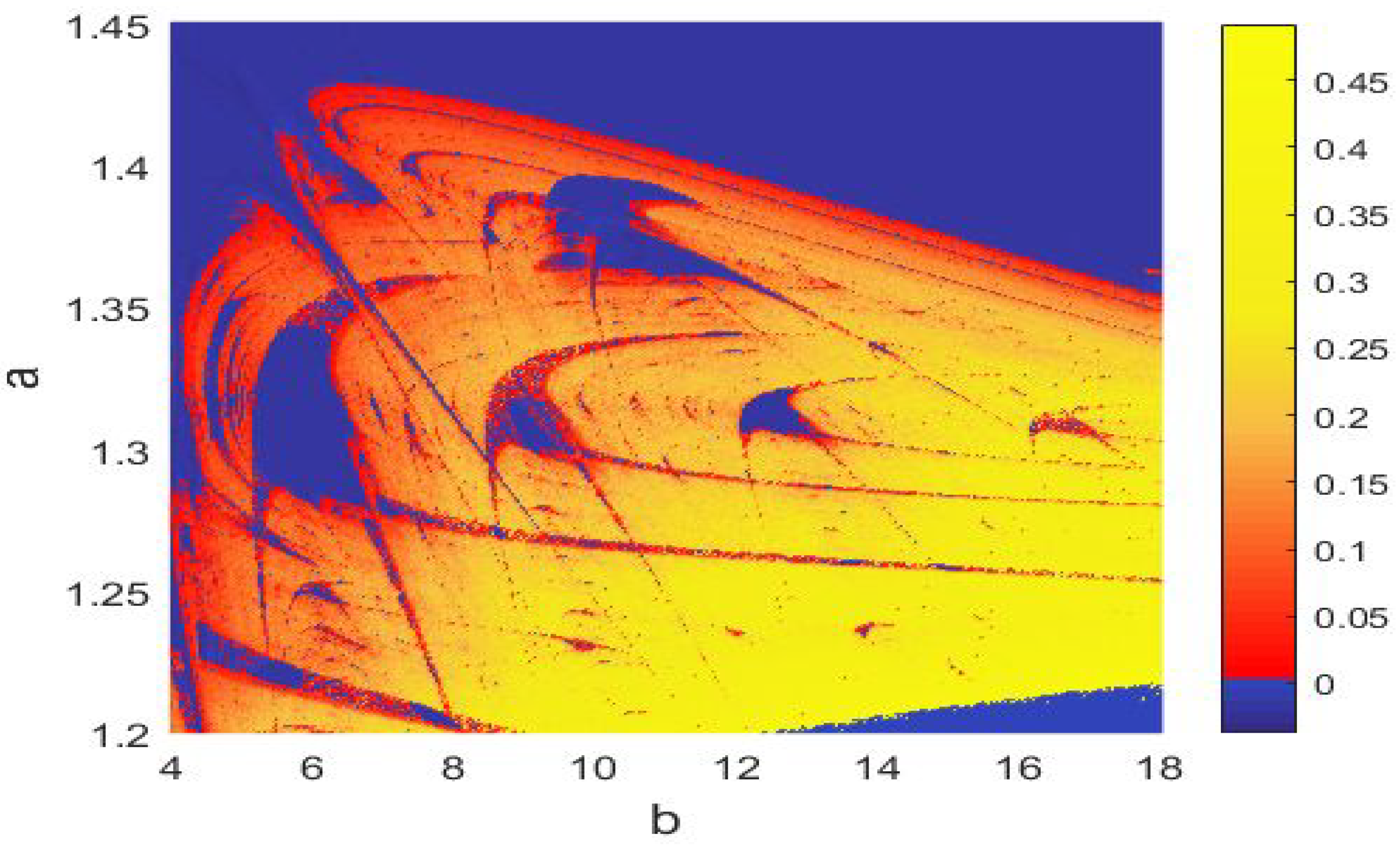
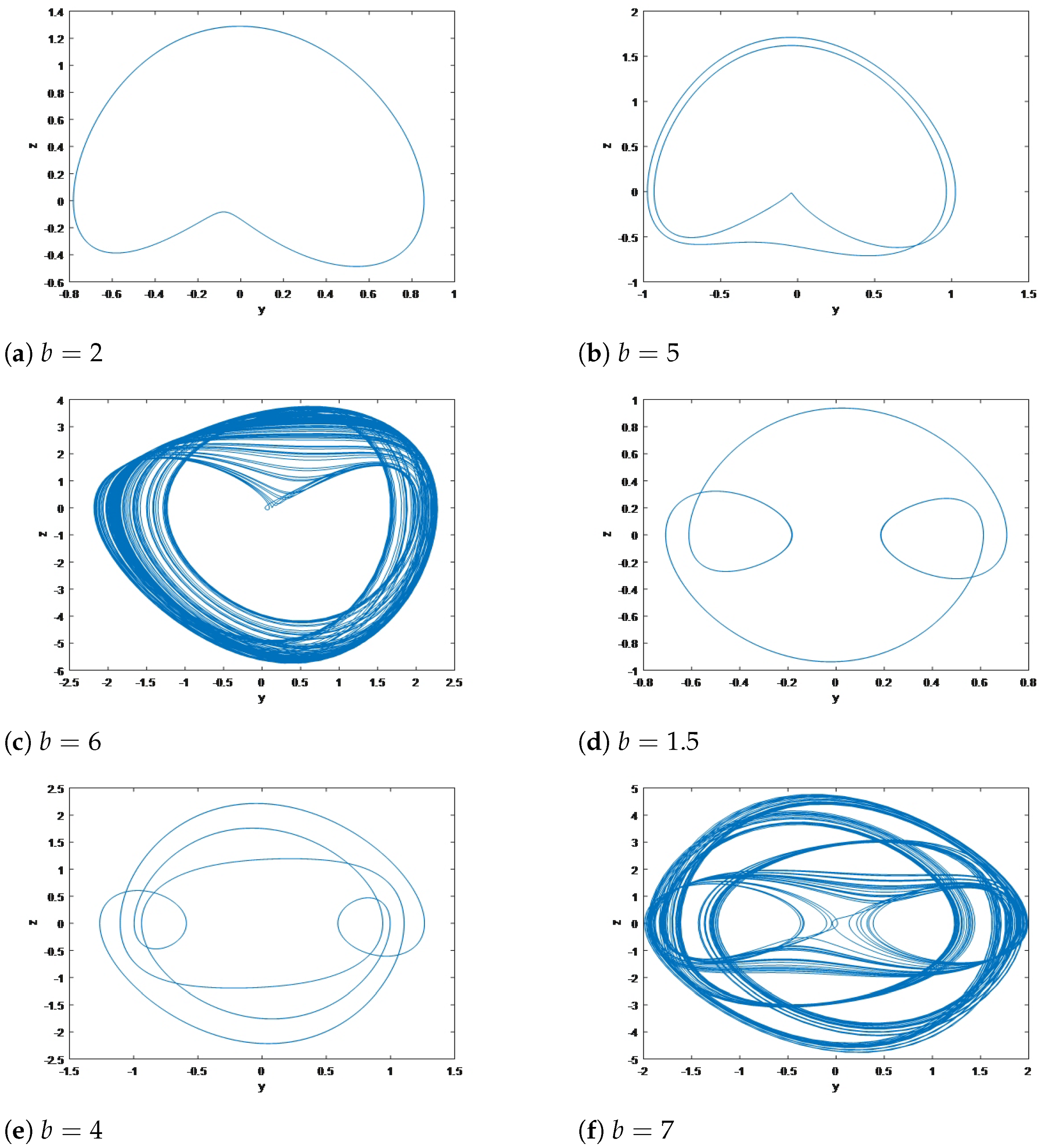
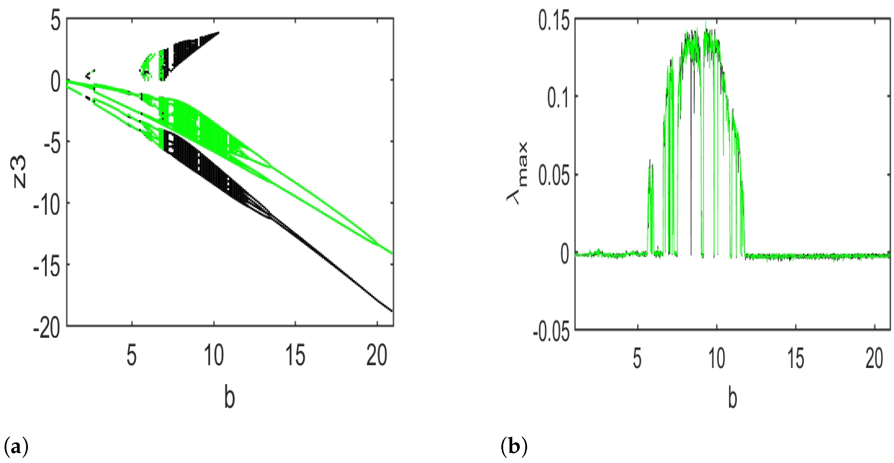
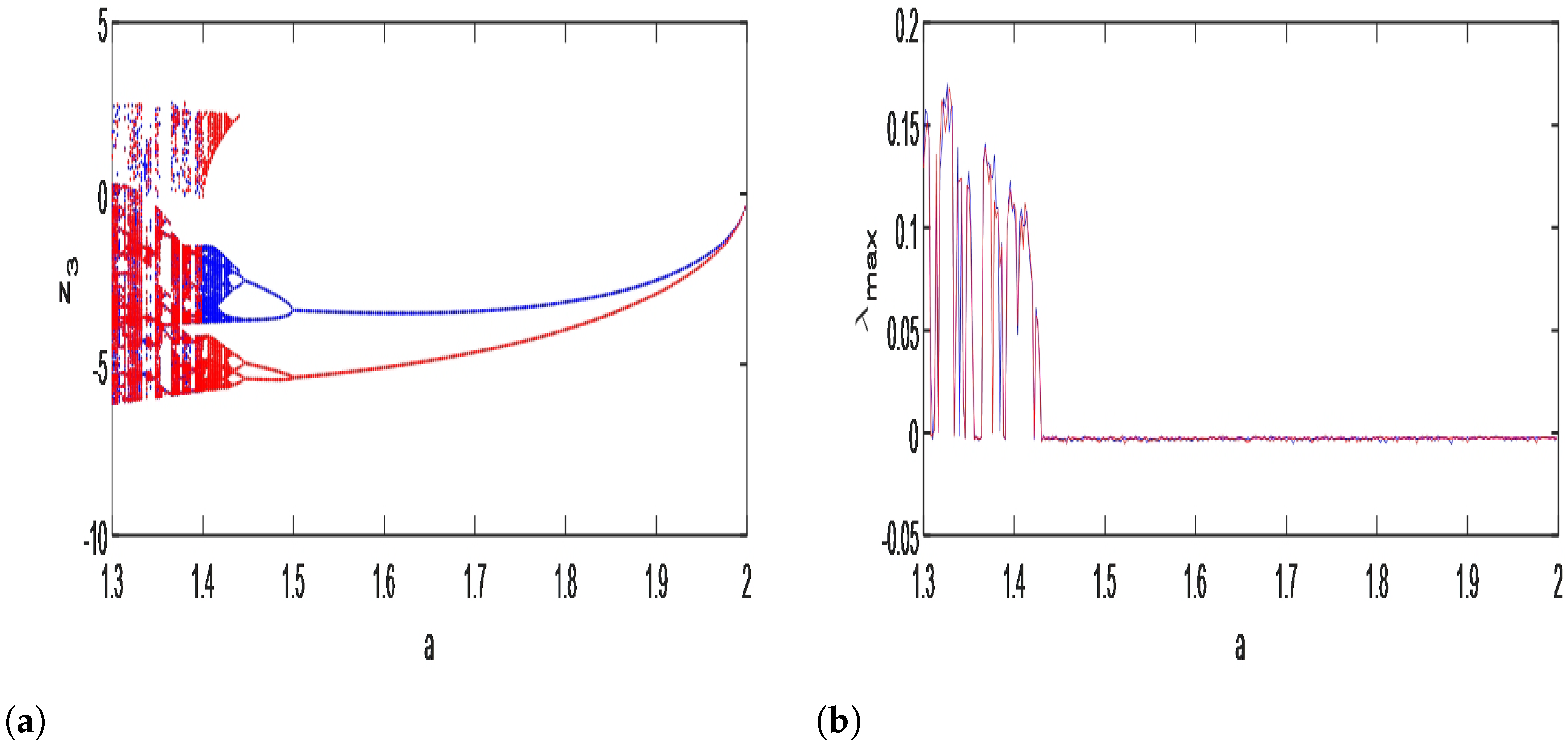
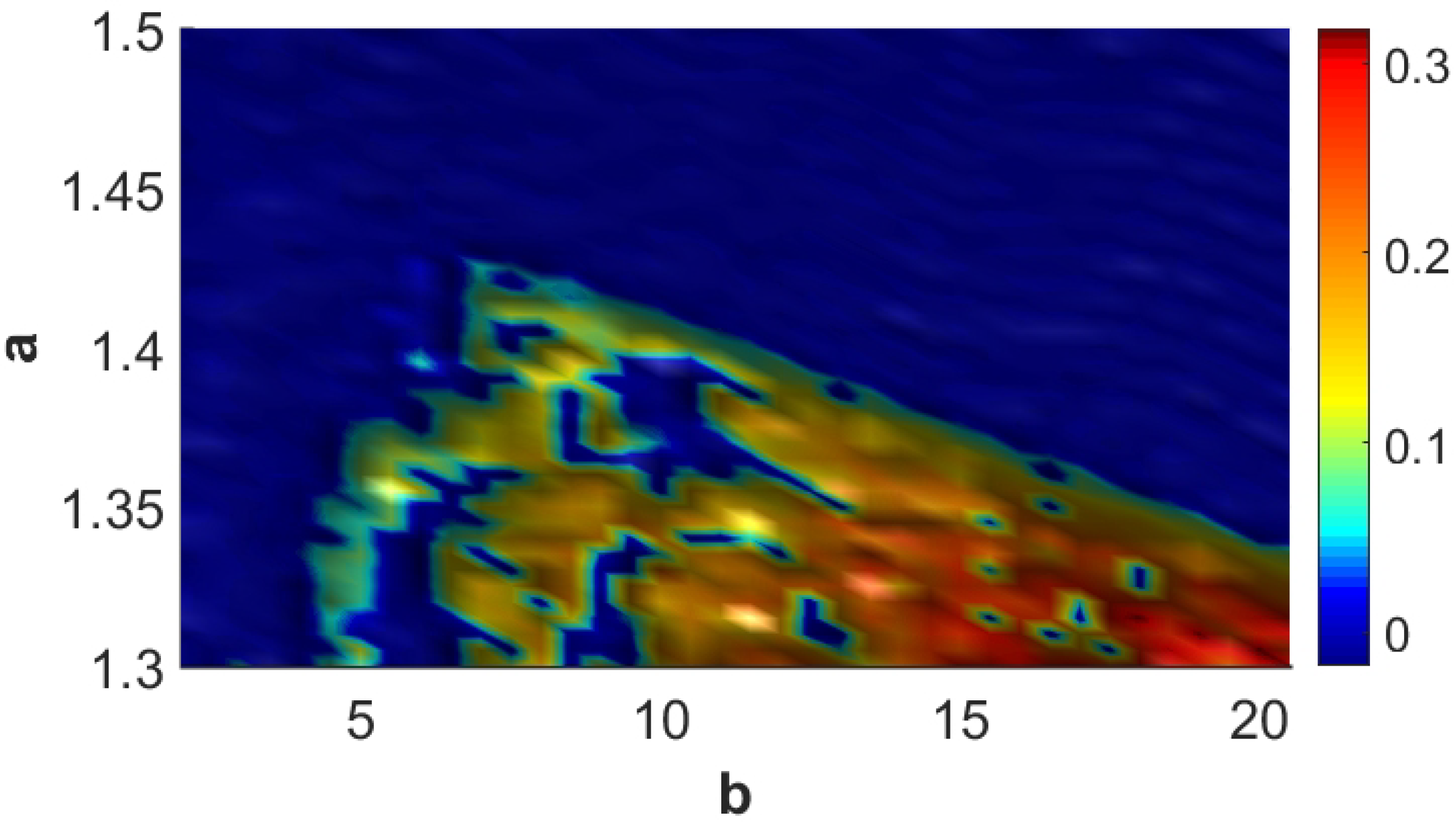
3. Bifurcation Analysis of the New Jerk System

To define different routes to chaos in our system and to investigate the rich behavior as a bifurcation diagram that can be spotted in the new jerk system in Equation (4), a numerical study is carried out using a standard fourth-order Runge–Kutta integration scheme technique. The dynamical study of our model starts by analyzing possible states of fixed points, their stability, and bifurcations that arrive under the control of corresponding parameters of model components.

For this bifurcation study of the jerk system (4), the time step is chosen such that $\mathsf{\Delta }t=0.005$ for every set of parameter values, and computations are carried out using variables and constant parameters in extended mode. For each setting, the jerk system (4) is integrated for a sufficiently long time, and the transitional phase is removed.

To call attention to the influence of the system parameters on the dynamics of the jerk system (4), we maintain that $a=1.4$ and b can be used as bifurcation parameters. Figure 3 supplies the bifurcation diagram of the coordinate $z_1$ versus b and the related plots of the largest Lyapunov exponent (${\lambda }_{max}$) of the jerk system (4) versus b. These figures are obtained by scanning the parameter downward without resetting the initial conditions, beginning the system from the initial state $(0.3,0.2,0.3)$. From Figure 3, we can observe very abundant and remarkable bifurcation scenarios. This bifurcation diagram shows that the jerk system is very sensitive to even a slight variation of the initial conditions. Chaotic motion is achieved progressively within the chaotic oscillator with respect to the control parameter b. Period-doubling bifurcation sequences and periodic windows can be easily identified in the graphs of Figure 3a,b.

Figure 4 shows the stability diagram for which the Lyapunov exponent band is activated for a better decision on the type of behavior. In light of Figure 3, behavior corresponds to a color and is confirmed by the values of the Lyapunov exponent. Thus, the data in blue are the behaviors of periodicities; those in red from $[0,2]$ represent low chaos, and those in yellow are higher chaos (expressing positive Lyapunov exponents). This spectrum is plotted when two parameters (a and b) vary at the same time. We remark that these Lyapunov stability diagrams are of paramount importance for the choice of parameters a and b, for better control of the system, as well as for a practical study (chaotic behavior is suitable for encryption, for example). This diagram is useful in choosing the range of parameters used in applications including chaos-based encryption.

Figure 5 shows many forms of attractors in the $(z_2,z_3)$ plane for the jerk system (4) when the parameter a is fixed at $a=1.4$ and the values of b are varied. For $b=2$, we obtain a limit cycle as shown in Figure 5a. For $b=5$, we obtain a period-2 attractor as shown in Figure 5b. For $b=6$, we obtain a chaotic attractor as shown in Figure 5c. The jerk system (4) exhibits a chaotic attractor for $a=1.4$ and for $6\le b\le 7$. Figure 5d–f show an abrupt change in the shape of the attractor of the jerk system (4) in the $(z_2,z_3)$ plane as b takes the values $b=1.5$, $b=4$ and $b=7$.

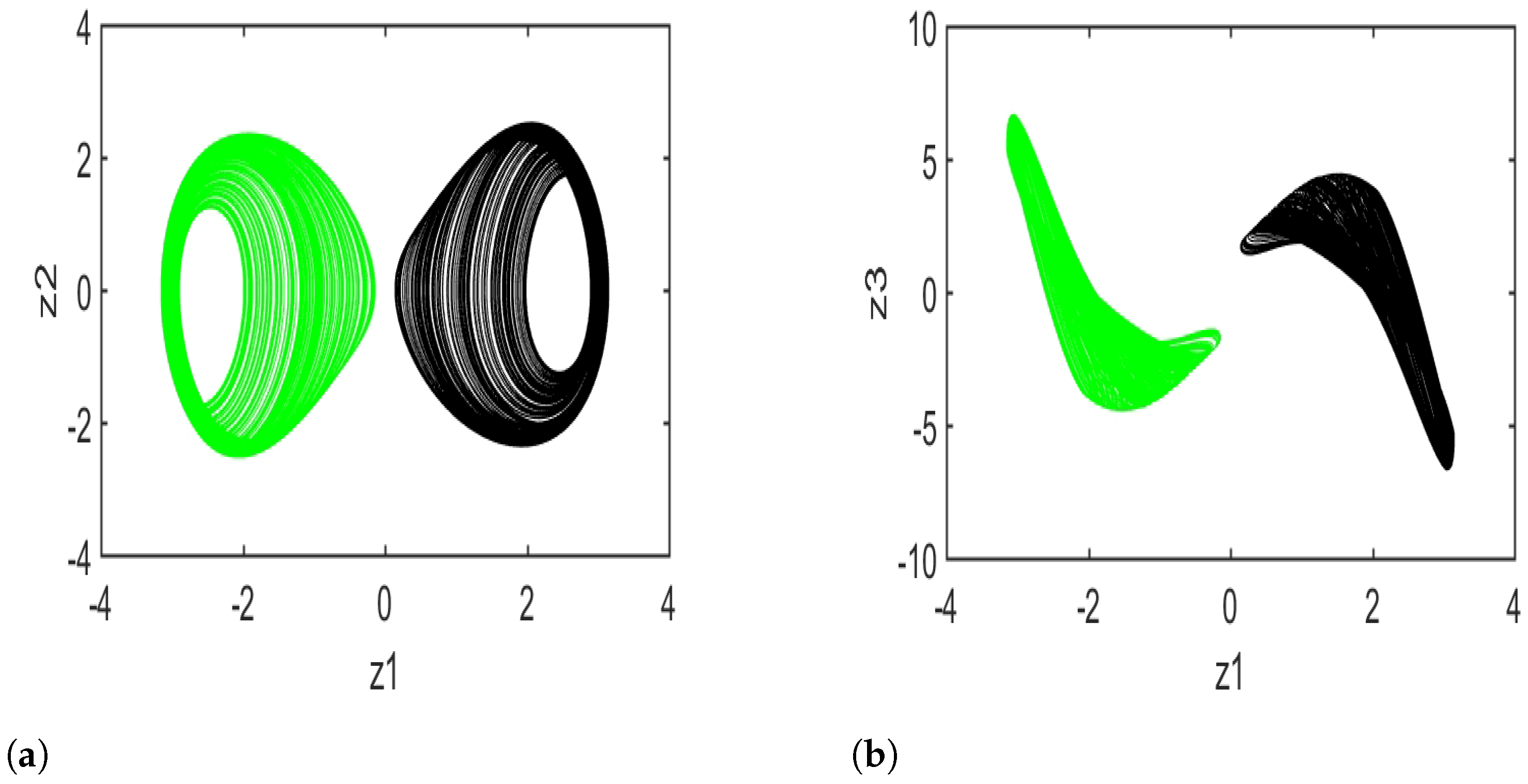
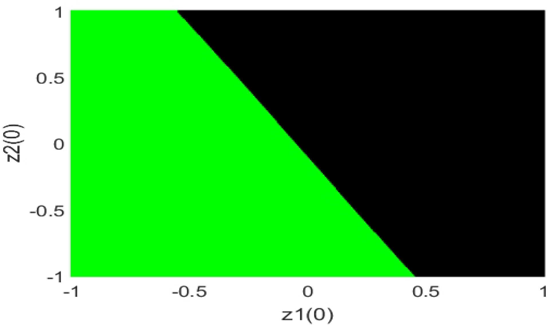
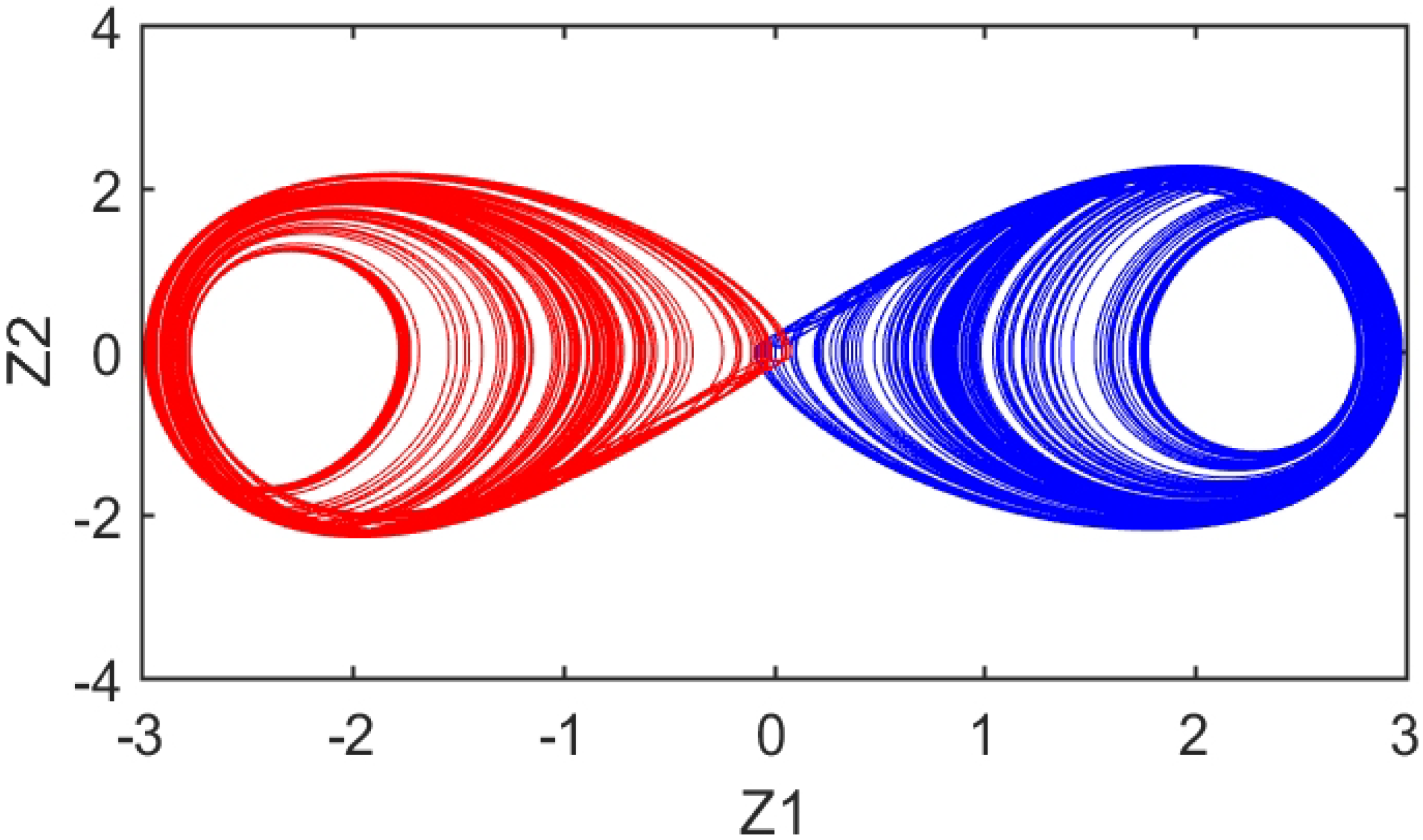
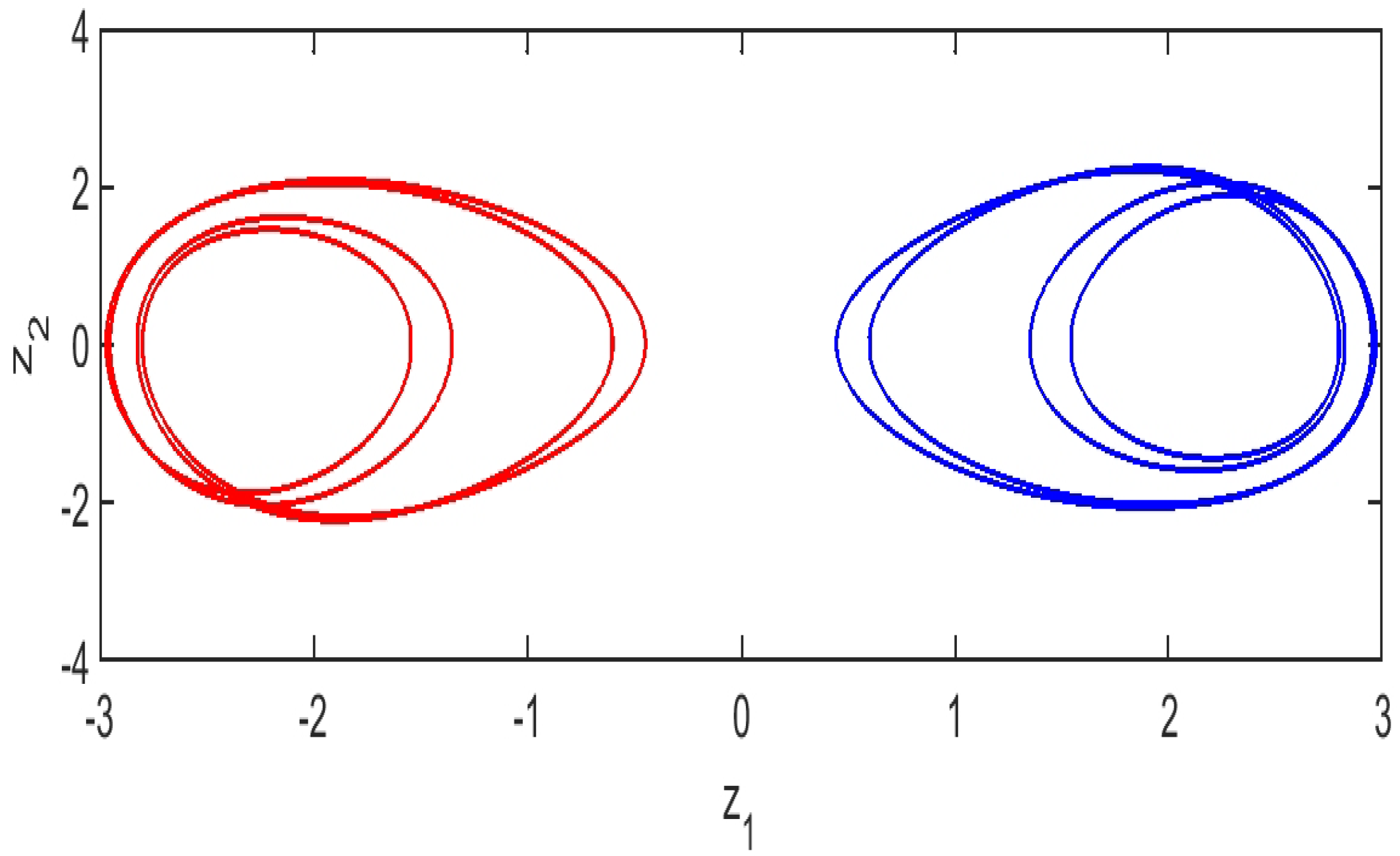
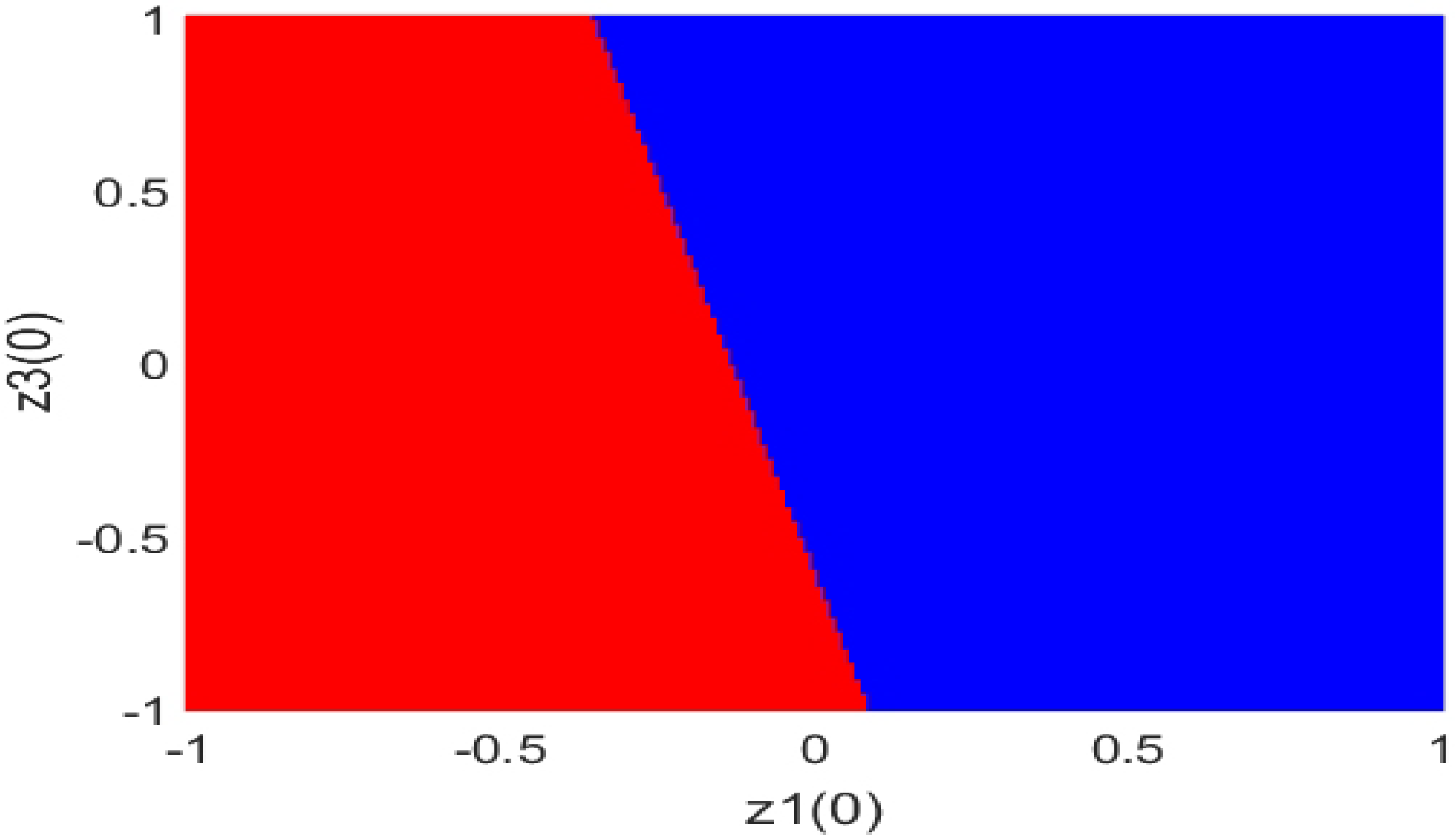
4. Multi-Stability and Coexistence of Attractors

An attractor is a domain of convergence of the evolutions (trajectories) of a system. A system can have several attractors. The coexistence of several attractors or multi-stability is another remarkable property of interactive systems with nonlinear regulation [33]. In numerical simulations, the variation of the initial conditions influences the dynamic behavior of the system. For the jerk system (4), we can observe multi-stability and verify the coexistence of attractors for the range of $8\le b\le 14$, when a is fixed at $a=1.4$. In this region, we observe the coexistence of two periodic period-2 attractors on the one hand and the coexistence of two chaotic attractors on the other hand. Figure 6 shows the bifurcation diagram and its corresponding maximum Lyapunov exponent (${\lambda }_{max}$) of the jerk system (4) scrolling forward (green) and backward (black) for the parameter b.

Figure 7 shows the presence of two different chaotic attractors for $a=1.4$ and $b=8$.

Figure 8 shows the presence of two different periodic attractors for $a=1.4$ and $b=14$.

Further information about the coexistence of the attractors can be obtained by analyzing the basins of attraction of the different attractors, which are defined as the set of initial conditions whose trajectories converge to the considered attractor. In order to understand the coexistence of attractors, the basin of attraction is studied. Let us take the coexisting periodic attractors of Figure 8. Their basin limits are clearly observed in Figure 9, showing the cross-section of the basin of attraction for $z_3=0.3$.

For studying the influence of the parameter a, we describe the bifurcation diagram and maximum Lyapunov exponent $\left({\lambda }_{max}\right)$ as shown on Figure 10.

Figure 10 shows the coexistence of multiple attractors for the jerk system (4). Taking the parameter $a=1.4$, the chaotic attractors coexist for the jerk system (4) as shown in Figure 11. Taking the parameter $a=1.44$, the periodic attractors coexist for the jerk system (4) as shown in Figure 12.

The basin of attraction corresponding to the chaotic attractors of Figure 11 is shown in Figure 13.

Figure 14 shows the two-parameter bifurcation diagram based on the sign of the maximum Lyapunov exponent $\left({\lambda }_{max}\right)$ for the jerk system (4).

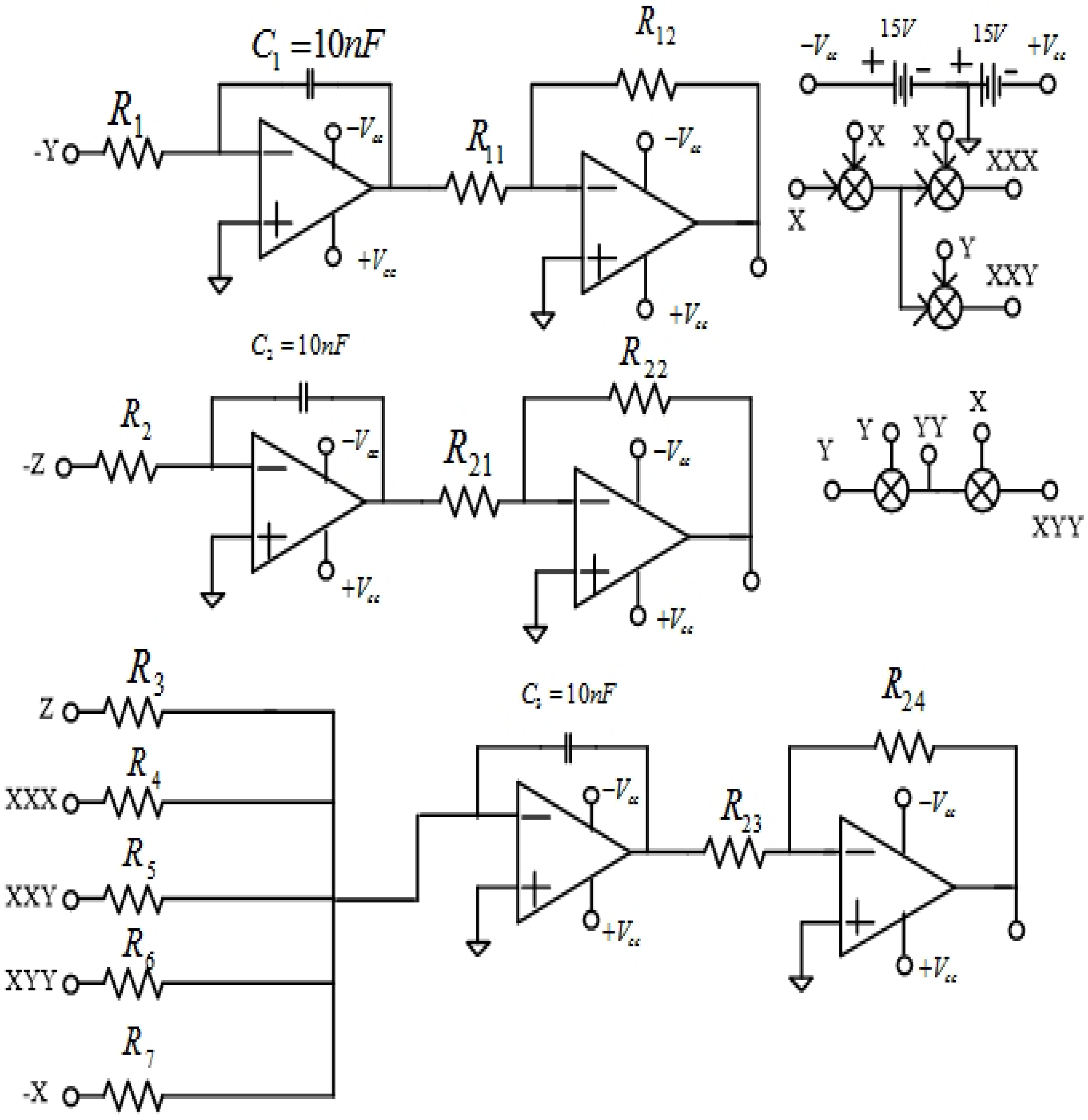
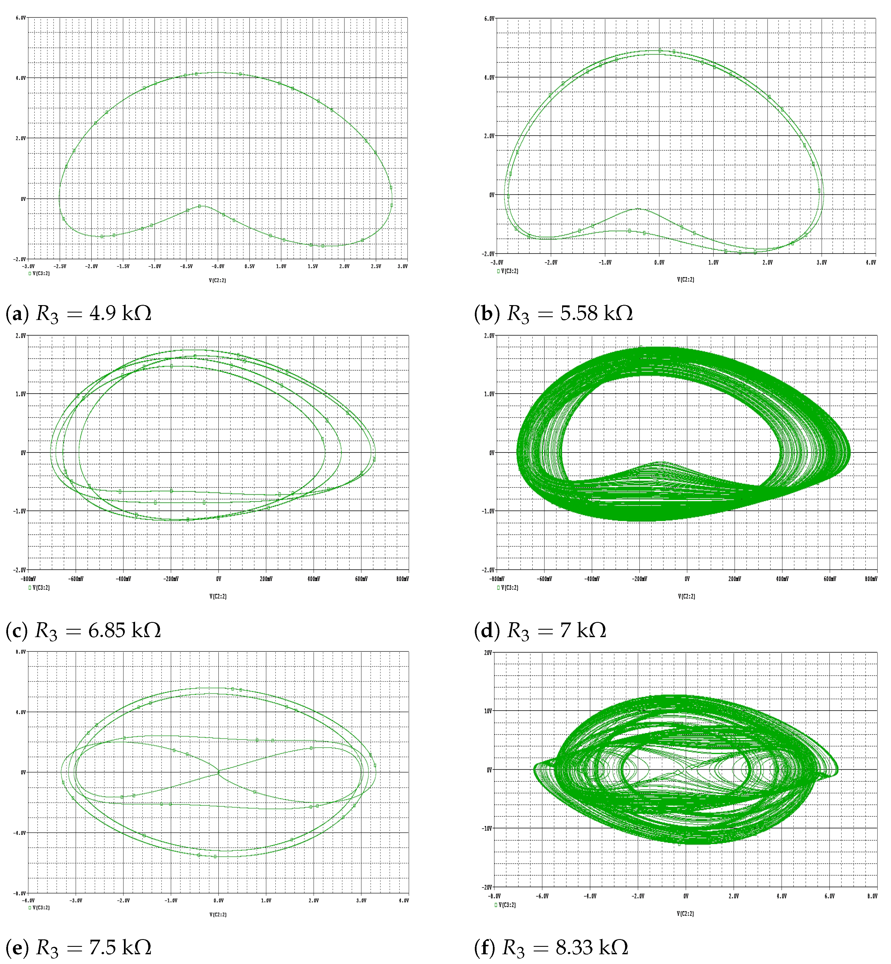
5. Circuit Simulation of the Jerk System

This section details the implementation of an electronic circuit that emulates the jerk system proposed in Equation (4) in PSPICE and performs a series of simulations in order to validate the mathematical model proposed from our circuit. On the other hand, it is interesting to evaluate the effects of the simplifying ideal operational amplifier assumptions adopted during the modeling process on the actual behavior of the oscillator in PSPICE. The circuit of Figure 15 is simulated in PSPICE with the values of the resistances equivalent to the parameters scaled in the numerical study to effectively verify the sensitivity of the model to the control parameter, which for us, will be the resistance from the modeling of the circuit equations.

The following circuit can be used to represent the jerk system (4) for an analogical study.

Using Kirchhoff’s circuit analysis laws for the proposed circuit in Figure 15, we derive the circuit model of the jerk system (4), which is described by the following equations:

$$\left\{\begin{array}{ccc}{V}_{S_1}& =& -\frac{1}{C_1}\int \frac{V_{S_2}}{R_1}dt\hfill \\ V_{S_2}& =& -\frac{1}{C_2}\int \frac{V_{S_3}}{R_2}dt\hfill \\ V_{S_3}& =& -\frac{1}{C_3}\int \left[\frac{V_{S_3}}{R_3}+\frac{V_{S_1}^3}{R_4}+\frac{V_{S_1}^2{V}_{S_2}^2}{R_5}\right.\hfill \\ & & \left.+\frac{V_{S_1}{V}_{S_2}^2}{R_5}+\frac{V_{S_1}{V}_{S_2}^2}{R_6}+\frac{V_{S_1}}{R_7}\right]dt\hfill \end{array}\right.$$

(14)

where $V_{S_i}$ correspond to the voltages.

Let $V_{S_i}=\alpha Z_i$, where $i=1,2,3$. Then, we obtain the following system of equations for the circuit model:

$$\left\{\begin{array}{ccc}\alpha \dot{Z_1}& =& -\frac{R}{R_1{C}_1}\alpha Z_2\hfill \\ \alpha \dot{Z_2}& =& -\frac{R}{R_2{C}_2}\alpha Z_3\hfill \\ \alpha \dot{Z_3}& =& -\frac{\alpha R}{C_3{R}_3}{Z}_3-\frac{{\alpha }^{3}R}{C_3{R}_4}{Z}_1^3-\frac{{\alpha }^{3}R}{C_3{R}_5}{Z}_1^2{Z}_2\hfill \\ & & -\frac{{\alpha }^{3}R}{C_3{R}_6}{Z}_1{Z}_2^2-\frac{\alpha R}{C_3{R}_7}{Z}_1\hfill \end{array}\right.$$

(15)

We can therefore suggest that the circuit model (15) is equivalent to the jerk system (4). The components of the circuit have been chosen to correspond to Equation (4). In particular, the parameter values can be set according to the following relationships.

By letting $\alpha =\sqrt{10}$, we observe that

$$a=\frac{\alpha }{R_3{C}_3},b=\frac{\alpha R}{R_7{C}_3},R={10}^{-4}$$

(16)

The values of the components of the circuit are given as follows:

$$R_1=R_2=10\mathrm{k}\mathsf{\Omega },R_4=R_5=R_6=1\mathrm{k}\mathsf{\Omega },R_7=1.428\mathrm{k}\mathsf{\Omega },$$

(17)

$$C_1=C_2=C_3=10\mathrm{nF}.$$

(18)

We vary the values of $R_3$ to obtain different phase portraits for the circuit model (15).

It is easy to see the good agreement between the MATLAB plots of the jerk system (4) and the simulation results of the circuit (15).

The following Figure 16 shows the various phase portraits of circuit (15) illustrating the route to chaos, where the initial values are taken as $Z\left(0\right)=(0.3,0.2,0.3)$.

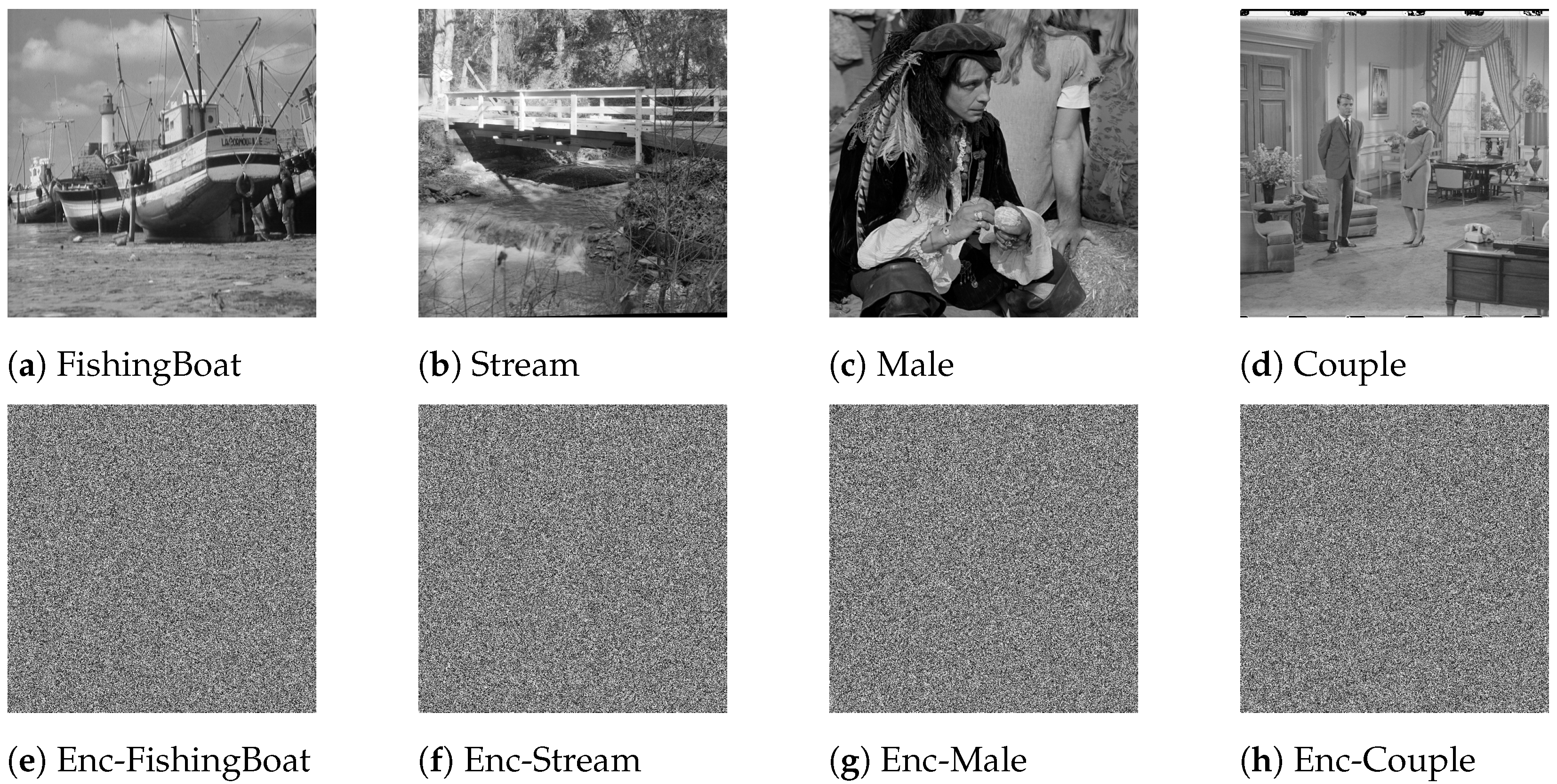
6. Encryption Algorithm and Its Performance

Because of their high sensitivity to primary conditions and their chaotic demeanor, chaotic systems are commonly utilized for developing image cryptosystems. In this section, we present the image encryption approach as a cryptographic application of the presented jerk system as well as the experimental results of this encryption mechanism.

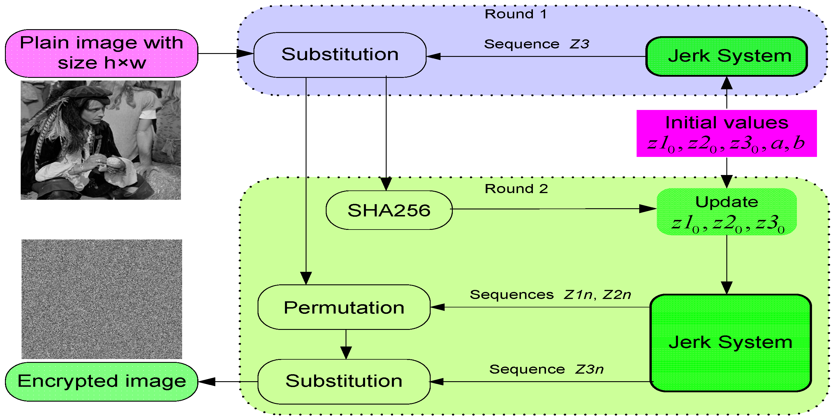
6.1. Proposed Encryption Algorithm

For making the presented cryptosystem applicable in real-time applications, the presented jerk system is required to be accommodated as stated in Equation (19).

$$\left\{\begin{array}{c}{z1}_{i+1}={z2}_i\hfill \\ {z2}_{i+1}={z3}_i\hfill \\ {z3}_{i+1}=\left(-a{z3}_i-{z1}_i({z1}_i^2+{z1}_i{z2}_i+{z2}_i^2-b)\right)mod1\hfill \end{array}\right.$$

(19)

The proposed encryption approach consists of two rounds of encryption. In the first round, the jerk system (19) is iterated $h\times w$ times using the initial conditions (${z1}_0$, ${z2}_0$, and ${z3}_0$) and control parameters (a and b) for generating three chaotic sequences ($\left\{Z1\right\}$, $\left\{Z2\right\}$, and $\left\{Z3\right\}$) in which $h\times w$ is the size of the plain image and sequence $\left\{Z3\right\}$ is utilized in the substitution process. In the second round, some information about the substituted image is gained by using the SHA-256 algorithm for modernizing the prime conditions of the jerk system (${z1}_0$, ${z2}_0$, and ${z3}_0$) and for iterating the jerk system for $h\times w$ times utilizing the updated primary conditions for generating new three chaotic sequences ($\left\{Z1n\right\}$, $\left\{Z2n\right\}$, and $\left\{Z3n\right\}$), in which $\left\{Z1n\right\}$ and $\left\{Z2n\right\}$ are used to construct two permutation boxes for permutating the substituted image. Sequence $\left\{Z3n\right\}$ is utilized to substitute the permutated image for constructing the final encrypted image. The general framework of the encryption process is given in Figure 17, while the steps of encryption are itemized as follows.

Step 1: Choose values for primary conditions (${z1}_0$, ${z2}_0$, and ${z3}_0$) and control parameters (a and b) for iterating our chaotic jerk system (19) $h\times w$ times to construct three chaos sequences $\left\{Z1\right\}$, $\left\{Z2\right\}$, and $\left\{Z3\right\}$. Here, $h\times w$ is the size of the original image OIm.

Step 2: Transform the elements of the sequence $\left\{Z3\right\}$ into integers in the range $[0,255]$, and reshape the output into a matrix $Key1$.

$$K1=floor(Z3\times {10}^{14})mod256$$

(20)

$$Key1=reshape(K1,h,w)$$

(21)

Step 3: Apply the bit XOR operation between the original image OIm and matrix $Key1$ to obtain the substituted image SbIm.

$$SbIm=OIm\oplus Key1$$

(22)

Step 4: Apply the SHA-256 hashing algorithm on the substituted image SbIm to obtain 256 bits (A), then those bits are converted into 32 integers (T), each of 8 bit, and then those integers are converted into three decimals ($M1$, $M2$, and $M3$) to update the initial values for ${z1}_0$, ${z2}_0$, and ${z3}_0$.

$$M1=\frac{t_1\oplus t_2\oplus \cdots \oplus t_{11}}{256}$$

(23)

$$M2=\frac{t_{12}\oplus t_{13}\oplus \cdots \oplus t_{22}}{256}$$

(24)

$$M3=\frac{t_{23}\oplus t_{24}\oplus \cdots \oplus t_{32}}{256}$$

(25)

$$\begin{array}{c}{z1}_{new}=\left(z{1}_0+M1\right)/\phantom{\left(z{1}_0+M1\right)2}2\hfill \\ {z2}_{new}=\left(z{2}_0+M2\right)/\phantom{\left(z{2}_0+M2\right)2}2\hfill \\ {z3}_{new}=\left(z{3}_0+M3\right)/\phantom{\left(z{3}_0+M3\right)2}2\hfill \end{array}$$

(26)

Step 5: Using the modernized initial conditions (${z1}_{new}$, ${z2}_{new}$, and ${z3}_{new}$) and the old control parameters (a and b), iterate our jerk system (19) $h\times w$ times to construct new three chaos sequences $\left\{Z1n\right\}$, $\left\{Z2n\right\}$, and $\left\{Z3n\right\}$.

Step 6: Arrange the first h elements of sequence $\left\{Z1n\right\}$ from the smallest to the largest to obtain vector $\left\{B\right\}$; then, obtain the index of every element of $\left\{Z1n\right(1:h\left)\right\}$ in $\left\{B\right\}$ as a permutation box $\left\{Ph\right\}$.

Step 7: Arrange the first w elements of sequence $\left\{Z2n\right\}$ from the smallest to the largest to obtain vector $\left\{D\right\}$; then, obtain the index of every element of $\left\{Z2n\right(1:w\left)\right\}$ in $\left\{D\right\}$ as a permutation box $\left\{Pw\right\}$.

Step 8: Permutate the substituted image SbIm using the permutation boxes $\left\{Ph\right\}$ and $\left\{Pw\right\}$.

$$\begin{array}{c}PrIm(x,y)=SbIm\left(Ph\right(x),Pw(y\left)\right),\\ forx=1,2,...,h\\ andy=1,2,...,w\end{array}$$

(27)

Step 9: Transform the elements of the sequence $\left\{Z3n\right\}$ into integers in the range $[0,255]$, and reshape the output into a matrix $Key2$.

$$K2=floor(Z3n\times {10}^{14})mod256$$

(28)

$$Key2=reshape(K2,h,w)$$

(29)

Step 10: Apply the bit XOR operation between the permutated image PrIm and matrix $Key2$ to obtain the final encrypted image EcIm.

$$EcIm=PrIm\oplus Key2$$

(30)

6.2. Performance Analysis

To evaluate the proposed encryption mechanism, we used MATLAB R2016b and a PC with an Intel(R) ${Core}^{TM}$2 Duo 3.00 GHz CPU and 4 GB of RAM. In addition, four standard test images with dimensions of $512\times 512$ were used as test images from the SIPI dataset [34] and were labeled as FishingBoat, Stream, Male, and Couple. The initial values of conditions and control parameters for running the jerk system (19) were set as: ${z1}_0=0.3$, ${z2}_0=0.2$, ${z3}_0=0.3$, $a=1.2$, and $b=2.5$. The visual effects of original images and their encrypted ones utilizing the suggested encryption algorithm and the declared key parameters are given in Figure 18, in which the encrypted images are completely noised.

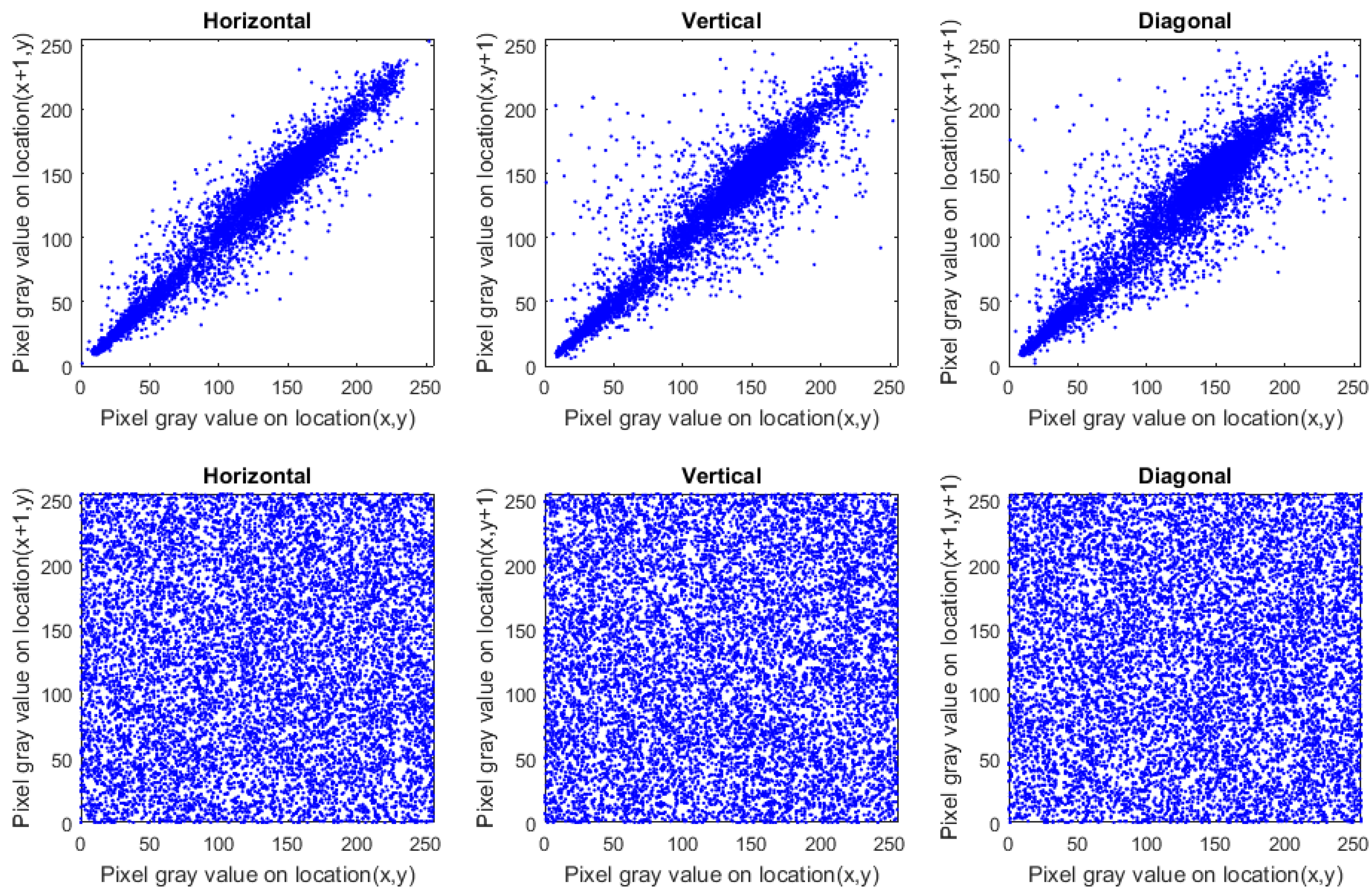
6.2.1. Correlation Analysis

The correlation coefficient, which is employed to determine the relationship between the pixels that exist in the image, is one of the essential tools used to estimate the meaning of the image. Correlation coefficient values of the original images are nearly 1 in each direction, but they should be near 0, with ciphered images using a good encryption mechanism (no relationship between the pixels that exist in the image) [35]. To calculate the correlation coefficients for the suggested encryption mechanism, we randomly selected 10,000 pairs of adjacent pixels in each direction.

Table 1. Outcomes of correlation coefficients.

Image	Direction
	H	V	D
FishingBoat	0.9703	0.9355	0.9143
Enc-FishingBoat	0.0006	−0.0004	0.0001
Stream	0.9265	0.9407	0.8985
Enc-Stream	0.0004	−0.0007	−0.0001
Male	0.9695	0.9615	0.9388
Enc-Male	0.0001	−0.0008	−0.0006
Couple	0.8836	0.9353	0.8542
Enc-Couple	−0.0001	−0.0009	−0.0005

shows the correlation coefficient results, which reveal that correlation values for encrypted images are extremely near to 0. Figure 19 depicts the correlation distribution of neighboring pixels in each direction for FishingBoat images before and after encryption. By analyzing the correlations of neighboring pixels, no significant information about the original image can be gleaned from the results stated in Table 1 and Figure 19.

6.2.2. Differential Analysis

To evaluate the suggested encryption approach against differential attacks, we performed NPCR (number of pixels change rate) and UACI (unified average changing intensity) tests [35], which are both defined as given below.

$$\begin{array}{c}NPCR=\frac{\sum _{i,j}f(x,y)}{T}\times 100\%,\\ f(x,y)=\left\{\begin{array}{c}0whenE1(x,y)=E2(x,y)\\ 1whenE1(x,y)\ne E2(x,y)\end{array}\right.\end{array}$$

(31)

$$UACI=\frac{1}{T}\left(\sum _{x,y}\frac{\left|E1(x,y)-E2(x,y)\right|}{255}\right)\times 100\%$$

(32)

where T points to the number of pixels that exist in the image, and $E1$ and $E2$ are two encrypted images for one original image with slight change in one bit.

Table 2. Results of NPCR and UACI.

Image	NPCR	UACI
FishingBoat	99.61738%	33.40942%
Stream	99.61395%	33.45551%
Male	99.61509%	33.53011%
Couple	99.62539%	33.44076%

displays the outcomes of the NPCR and UACI tests, with the average NPCR value being >99.6%. As a result, the presented encryption method is extremely sensitive to minor pixel changes in the original image.

6.2.3. Histogram Analysis

The frequency of pixel values in an image is shown by the histogram test, which is a crucial statistic for measuring the effectiveness of any encryption scheme. To resist statistical assaults, any effective encryption method must have identical histograms for various encrypted images. Figure 20 depicts the histograms of the original images that differ from one another, but the histograms of analog-encrypted images are similar. As well, the frequency distribution of pixel values in the encrypted image is measured using the chi-square test [35], which is a quantitative tool that is used to verify the regular distribution. The results of the chi-square test are provided in

Table 3. Results of chi-square.

Image	Chi-Square Value	Result
FishingBoat	383,969.6875	Varying
Stream	1,185,618.3476	Varying
Male	158,413.5429	Varying
Couple	298,865.2441	Varying
Enc-FishingBoat	245.4551	Uniform
Enc-Stream	227.9434	Uniform
Enc-Male	279.8770	Uniform
Enc-Couple	246.9727	Uniform

, in which all chi-square values for encrypted images are less than the threshold of 293. As a result, our technique of encryption can survive histogram assaults.

6.2.4. Information Entropy

Information entropy is a statistical measure that evaluates the distribution of bits per level in an image. To calculate the information entropy, the following formula can be used.

$$E\left(X\right)=-\sum _{i=1}^{255}p\left(v_i\right){log}_2\left(p\left(v_i\right)\right)$$

(33)

where $p\left(v_i\right)$ points to the probability of $v_i$. The potential values for pixels existing in a greyscale image are in [0,255], and thus, the perfect entropy value is 8 bit. As a result, to ensure the efficiency of the suggested encryption method, the entropy values should be close to 8. The results of information entropy for the original images and their encrypted counterparts are shown in

Table 4. The outcome of information entropy.

Image	Encrypted	Original
FishingBoat	7.999325	7.191370
Stream	7.999372	5.705560
Male	7.999229	7.534507
Couple	7.999321	7.201008

, where the entropy values for ciphered images are quite near to 8.

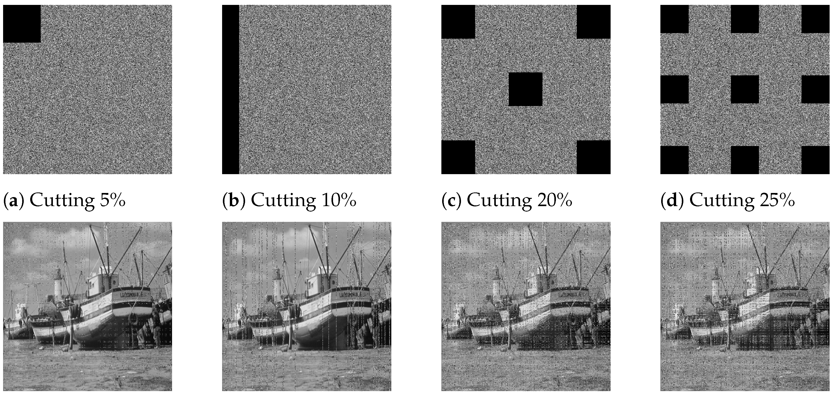
6.2.5. Occlusion Attack

It is possible to lose a portion of the transferred data while transmitting data across noisy carriers. As a result, a robust encryption technique must survive data loss assaults. To test our strategy against data loss threats, we remove some portions of the encrypted image and then attempt to decrypt it. Figure 21 depicts the outcome of the occlusion attack in which the original image is successfully recovered with no wasted information in the cutting portion position.

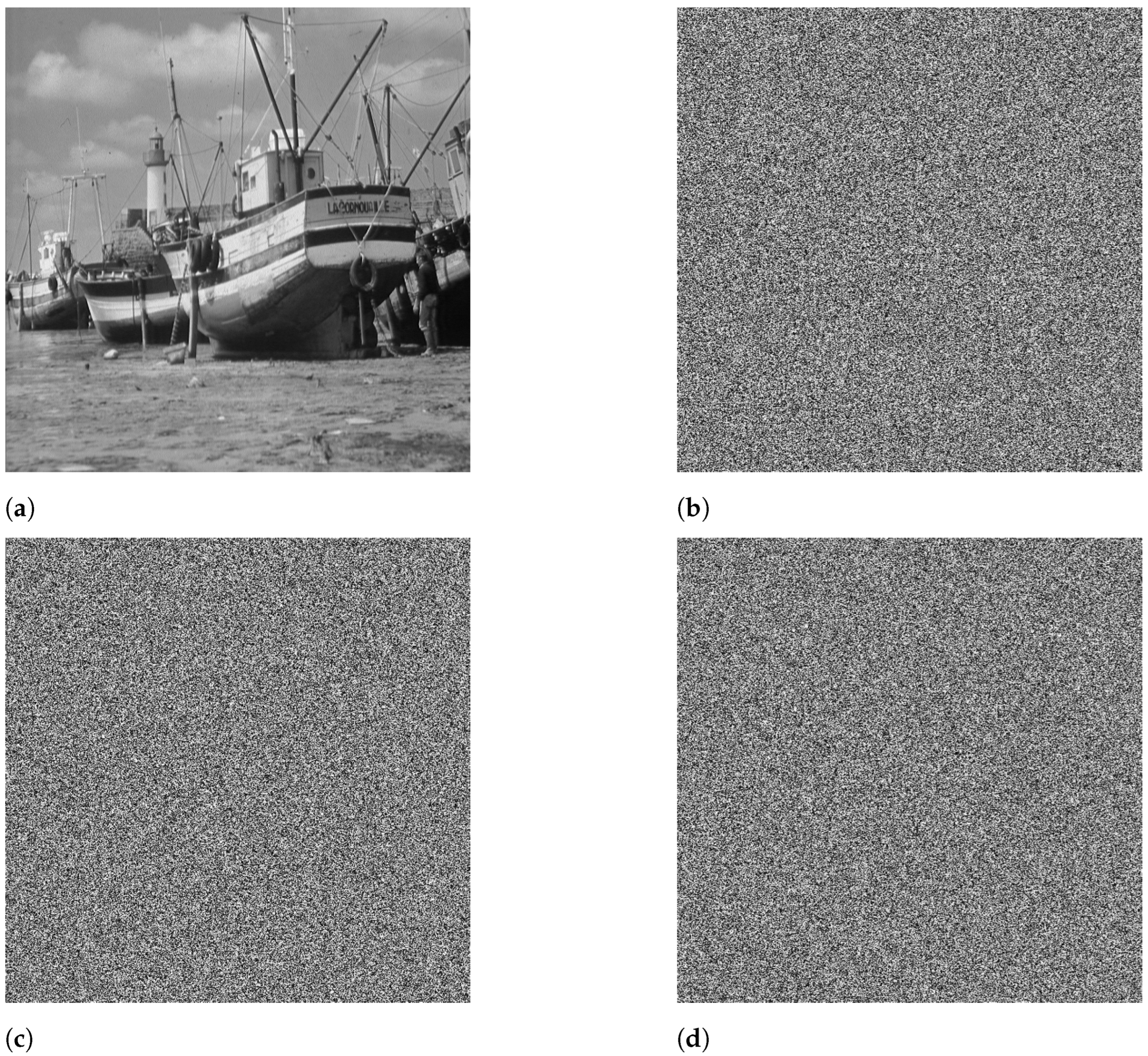
6.2.6. Key Sensitivity

Key sensitivity is an essential criterion for any robust encryption scheme. Any tiny modifications in key parameters lead to significant variations in the decrypted image. To test the key sensitivity of our proposed technique, we performed decryption on the Enc-FishingBoat image with various keys, as shown in Figure 22. From the results stated in Figure 22, any tiny modification in key parameters results in significant variations in the decrypted image.

7. Conclusions

In this paper, we presented a new chaotic jerk system with three cubic nonlinear terms. We conducted a qualitative study of the proposed jerk system and analyzed the stability properties of the three equilibrium points of the jerk system. We showed that the equilibrium points are unstable. Thus, the new chaotic jerk system has a self-excited chaotic attractor. The bifurcation structures of the proposed jerk system were investigated numerically, showing period-doubling, periodic windows and coexisting bifurcations. We used PSpice to carry out an electronic circuit simulation of the proposed jerk system. Circuit simulations of mathematical models using PSpice have their own limitations, as these simulations are based on simplified mathematical models. Finally, a new image-encryption approach was proposed based on the chaotic behavior of the presented jerk system. Experimental outcomes demonstrated that the suggested encryption approach is effective with high plain-image sensitivity and the reliability of the proposed chaotic jerk system for various cryptographic purposes. In the future, we plan to design an experimental realization of the proposed chaotic jerk system using a field-programmable gate array (FPGA).

References

1. Njimah, O.M.; Ramadoss, J.; Telem, A.N.K.; Kengne, J.; Rajagopal, K. Coexisting oscillations and four-scroll chaotic attractors in a pair of coupled memristor-based Duffing oscillators: Theoretical analysis and circuit simulation. Chaos Solitons Fractals 2023, 166, 112983. [Google Scholar] [CrossRef]
2. Aggarwal, B.; Rai, S.K.; Sinha, A. New memristor-less, resistor-less, two-OTA based grounded and floating meminductor emulators and their applications in chaotic oscillators. Integration 2023, 88, 173–184. [Google Scholar] [CrossRef]
3. Fan, W.; Chen, X.; Wu, H.; Li, Z.; Xu, Q. Firing patterns and synchronization of Morris-Lecar neuron model with memristive autapse. AEU—Int. J. Electron. Commun. 2023, 158, 154454. [Google Scholar] [CrossRef]
4. Messadi, M.; Kemih, K.; Moysis, L.; Volos, C. A new 4D Memristor chaotic system: Analysis and implementation. Integration 2023, 88, 91–100. [Google Scholar] [CrossRef]
5. Zhong, D.Z.; Zhao, K.K.; Hu, Y.L.; Zhang, J.B.; Deng, W.A.; Hou, P. Four-channels optical chaos secure communications with the rate of 400 Gb/s using optical reservoir computing based on two quantum dot spin-VCSELs. Opt. Commun. 2023, 529, 129109. [Google Scholar] [CrossRef]
6. Xu, X.; Krisnanda, T.; Liew, T.C.H. Limit cycles and chaos in the hybrid atom-optomechanics system. Sci. Rep. 2022, 12, 15288. [Google Scholar] [CrossRef] [PubMed]
7. Ramamoorthy, R.; Tsafack, N.; Saeed, N.; Kingni, S.T.; Rajagopal, K. Current modulation based vertical cavity surface emitting laser: System-on-chip realization and compressive sensing based image encryption. Opt. Quantum Electron. 2023, 55, 91. [Google Scholar] [CrossRef]
8. Gomes, I.; Korneta, W.; Stavrinides, S.G.; Picos, R.; Chua, L.O. Experimental observation of chaotic hysteresis in Chua’s circuit driven by slow voltage forcing. Chaos Solitons Fractals 2023, 166, 112927. [Google Scholar] [CrossRef]
9. Wang, Z.; Parastesh, F.; Tian, H.; Jafari, S. Symmetric synchronization behavior of multistable chaotic systems and circuits in attractive and repulsive couplings. Integration 2023, 89, 37–46. [Google Scholar] [CrossRef]
10. Shah, N.A.; Ahmed, I.; Asogwa, K.K.; Zafar, A.A.; Weera, W.; Akgül, A. Numerical study of a nonlinear fractional chaotic Chua’s circuit. AIMS Math. 2023, 8, 1636–1655. [Google Scholar] [CrossRef]
11. Ni, Y.; Wang, Z. Intermittent sampled-data control for exponential synchronization of chaotic delayed neural networks via an interval-dependent functional. Expert Syst. Appl. 2023, 223, 119918. [Google Scholar] [CrossRef]
12. Sun, J.; Mao, T.; Wang, Y. Solution of simultaneous higher order equations based on DNA strand displacement circuit. IEEE Trans. NanoBiosci. 2022, 21, 511–519. [Google Scholar] [CrossRef] [PubMed]
13. Gao, S.; Wu, R.; Wang, X.; Liu, J.; Li, Q.; Tang, X. EFR-CSTP: Encryption for face recognition based on the chaos and semi-tensor product theory. Inf. Sci. 2023, 621, 766–781. [Google Scholar] [CrossRef]
14. Rashid, A.A.; Hussein, K.A. Image encryption algorithm based on the density and 6D logistic map. Int. J. Electr. Comput. Eng. 2023, 13, 1903–1913. [Google Scholar] [CrossRef]
15. Alemami, Y.; Mohamed, M.A.; Atiewi, S. Advanced approach for encryption using advanced encryption standard with chaotic map. Int. J. Electr. Comput. Eng. 2023, 13, 1708–1723. [Google Scholar] [CrossRef]
16. Ding, S.; Wang, N.; Bao, H.; Chen, B.; Wu, H.; Xu, Q. Memristor synapse-coupled piecewise-linear simplified Hopfield neural network: Dynamics analysis and circuit implementation. Chaos Solitons Fractals 2023, 166, 112899. [Google Scholar] [CrossRef]
17. Xu, Q.; Chen, X.; Chen, B.; Wu, H.; Li, Z.; Bao, H. Dynamical analysis of an improved FitzHugh-Nagumo neuron model with multiplier-free implementation. Nonlinear Dyn. 2023, 111, 8737–8749. [Google Scholar] [CrossRef]
18. Vaidyanathan, S.; Benkouider, K.; Sambas, A. A new multistable jerk chaotic system, its bifurcation analysis, backstepping control-based synchronization design and circuit simulation. Arch. Control Sci. 2022, 32, 123–152. [Google Scholar]
19. Wang, Q.; Tian, Z.; Wu, X.; Tan, W. Coexistence of Multiple Attractors in a Novel Simple Jerk Chaotic Circuit with CFOAs Implementation. Front. Phys. 2022, 10, 835188. [Google Scholar] [CrossRef]
20. Chase Harrison, R.; Rhea, B.K.; Oldag, A.R.; Dean, R.N.; Perkins, E. Experimental Validation of a Chaotic Jerk Circuit Based True Random Number Generator. Chaos Theory Appl. 2022, 4, 64–70. [Google Scholar] [CrossRef]
21. Kamdem Tchiedjo, S.; Kamdjeu Kengne, L.; Kengne, J.; Djuidje Kenmoe, G. Dynamical behaviors of a chaotic jerk circuit based on a novel memristive diode emulator with a smooth symmetry control. Eur. Phys. J. Plus 2022, 137, 90. [Google Scholar] [CrossRef]
22. Gakam Tegue, G.; Nkapkop, J.; Tsafack, N.; Abdel, M.; Kengne, J.; Ahmad, M.; Jiang, D.; Effa, J.; Tamba, J. A novel image encryption scheme based on compressive sensing, elliptic curves and a new jerk oscillator with multistability. Phys. Scr. 2022, 97, 125215. [Google Scholar] [CrossRef]
23. Ramakrishnan, B.; Welba, C.; Chamgoué, A.C.; Karthikeyan, A.; Kingni, S.T. Autonomous jerk oscillator with sine nonlinearity and logistic map for sEMG encryption. Phys. Scr. 2022, 97, 095211. [Google Scholar] [CrossRef]
24. Sprott, J.C. Some simple chaotic jerk functions. Am. J. Phys. 1997, 65, 537–543. [Google Scholar] [CrossRef]
25. Sun, K.H.; Sprott, J.C. A simple jerk system with piecewise exponential nonlinearity. Int. J. Nonlinear Sci. Numer. Simul. 2000, 10, 1443–1450. [Google Scholar] [CrossRef]
26. Liu, M.; Sang, B.; Wang, N.; Ahmad, I. Chaotic dynamics by some quadratic jerk systems. Axioms 2021, 10, 227. [Google Scholar] [CrossRef]
27. Vaidyanathan, S.; Volos, C.K.; Kyprianidis, I.M.; Stouboulos, I.N.; Pham, V.T. Analysis, adaptive control and anti-synchronization of a six-term novel jerk chaotic system with two exponential nonlinearities and its circuit simulation. J. Eng. Sci. Technol. Rev. 2021, 8, 24–36. [Google Scholar] [CrossRef]
28. Rajagopal, K.; Pham, V.T.; Tahir, F.R.; Akgul, A.; Abdolmohammadi, H.R.; Jafari, S. A chaotic jerk system with non-hyperbolic equilibrium: Dynamics, effect of time delay and circuit realisation. Pramana—J. Phys. 2018, 90, 52. [Google Scholar] [CrossRef]
29. Abd-El-Atty, B. A robust medical image steganography approach based on particle swarm optimization algorithm and quantum walks. Neural Comput. Appl. 2023, 35, 773–785. [Google Scholar] [CrossRef]
30. Kaur, M.; Singh, S.; Kaur, M. Computational Image Encryption Techniques: A Comprehensive Review. Math. Probl. Eng. 2021, 2021, 5012496. [Google Scholar] [CrossRef]
31. Kumari, M.; Gupta, S. Performance comparison between Chaos and quantum-chaos based image encryption techniques. Multimed. Tools Appl. 2021, 80, 33213–33255. [Google Scholar] [CrossRef] [PubMed]
32. Pham, V.T.; Vaidyanathan, S.; Volos, C.; Kapitaniak, T. Nonlinear Dynamical Systems with Self-Excited and Hidden Attractors; Springer: New York, NY, USA, 2018. [Google Scholar]
33. Xu, Q.; Cheng, S.; Ju, Z.; Chen, M.; Wu, H. Asymmetric coexisting bifurcations and multi-stability in an asymmetric memristive diode-bridge-based jerk circuit. Chin. J. Phys. 2021, 70, 69–81. [Google Scholar] [CrossRef]
34. Kumlu, D. USC-SIPI REPORT# 422 2012. Available online: https://sipi.usc.edu/database/database.php?volume=misc (accessed on 5 February 2023).
35. Benkouider, K.; Vaidyanathan, S.; Sambas, A.; Tlelo-Cuautle, E.; El-Latif, A.A.A.; Abd-El-Atty, B.; Bermudez-Marquez, C.F.; Sulaiman, I.M.; Awwal, A.M.; Kumam, P. A New 5-D Multistable Hyperchaotic System With Three Positive Lyapunov Exponents: Bifurcation Analysis, Circuit Design, FPGA Realization and Image Encryption. IEEE Access 2022, 10, 90111–90132. [Google Scholar] [CrossRef]
Figure 1. Lyapunov exponents for the new jerk system (4) calculated using the simulation time T = 1 × 10 5 s for ( a , b ) = ( 1.2 , 2.5 ) and Z ( 0 ) = ( 0.3 , 0.2 , 0.3 ) .
Electronics 12 02818 g001
Figure 2. MATLAB simulations of the jerk system (4) for Z ( 0 ) = ( 0.3 , 0.2 , 0.3 ) and ( a , b ) = ( 1.2 , 2.5 ) : (a) ( z 1 , z 2 ) plane, (b) ( z 2 , z 3 ) plane, (c) ( z 1 , z 3 ) plane and (d) R 3 .
Electronics 12 02818 g002
Figure 3. (a) Bifurcation diagram of the jerk system (4) for z 1 versus b and (b) largest Lyapunov exponent ( λ max ) of the jerk system (4) versus b.
Electronics 12 02818 g003
Figure 4. Standard Lyapunov stability diagram plot for the jerk system (4) where two control parameters a and b vary at the same time. Each color corresponds to a behavior different from the blue color, which symbolizes the periodicities, red symbolizes low chaos, and yellow symbolizes the higher chaos.
Electronics 12 02818 g004
Figure 5. Attractors of the jerk system (4) in the ( z 2 , z 3 ) plane for Z ( 0 ) = ( 0.3 , 0.2 , 0.3 ) , a = 1.4 and various values of b.
Electronics 12 02818 g005
Figure 6. (a) Bifurcation diagram and the corresponding largest Lyapunov exponent for the jerk system (4) with the initial value Z ( 0 ) = ( 0.3 , 0.2 , 0.3 ) and a = 1.4 , and (b) Lyapunov spectrum.
Electronics 12 02818 g006
Figure 7. Coexistence of two different chaotic attractors of the jerk system (4) for the parameters a = 1.4 and b = 8 taking initial values ( 0.3 , 0.2 , 0.3 ) for the: (a) black attractor and (b) ( 0.3 , 0.2 , 0.3 ) for the green attractor.
Electronics 12 02818 g007
Figure 8. Coexistence of two different periodic attractors of the jerk system (4) for the parameters a = 1.4 and b = 14 taking initial values ( 0.1 , 0.1 , 0.3 ) for the black attractor and ( 0.1 , 0.4 , 0.3 ) for the green attractor.
Electronics 12 02818 g008
Figure 9. Basin of attraction of the jerk system (4) corresponding to Figure 8 for z 3 = 0.3 .
Electronics 12 02818 g009
Figure 10. (a) Bifurcation diagram and (b) the corresponding largest Lyapunov exponent for the jerk system (4) with the initial value Z ( 0 ) = ( 0.3 , 0.2 , 0.3 ) and b = 7 for the forward (blue) and backward (red) sweeping of the parameter a.
Electronics 12 02818 g010
Figure 11. Coexistence of two different chaotic attractors of the jerk system (4) for the parameter a = 1.4 and b = 8 taking initial values ( 0.3 , 0.2 , 0.3 ) for the blue attractor and ( 0.3 , 0.2 , 0.3 ) for the red attractor.
Electronics 12 02818 g011
Figure 12. Coexistence of two different periodic attractors of the jerk system (4) for the parameter a = 1.44 and b = 7 taking initial values ( 0.3 , 0.2 , 0.3 ) for the blue attractor and ( 0.2 , 0.2 , 0.3 ) for the red attractor.
Electronics 12 02818 g012
Figure 13. Basin of attraction of the jerk system (4) corresponding to Figure 11 for z 2 = 0.2 .
Electronics 12 02818 g013
Figure 14. Two parameter bifurcation diagram based on the sign of the maximum Lyapunov exponent ( λ max ) for the jerk system (4).
Electronics 12 02818 g014
Figure 15. Circuit diagram designed for the proposed jerk system (4).
Electronics 12 02818 g015
Figure 16. Phase portraits illustrating the route to chaos for the circuit model (15) for various values of R 3 .
Electronics 12 02818 g016
Figure 17. Outline of our encryption mechanism.
Electronics 12 02818 g017
Figure 18. Original images and their encrypted ones using the suggested encryption algorithm and the stated key parameters.
Electronics 12 02818 g018
Figure 19. Correlation distribution for Fishing Boat images before and after encryption, with the first row displaying the original image’s correlation distribution and the second row displaying the encrypted image’s correlation distribution.
Electronics 12 02818 g019
Figure 20. Histograms of plain and cipher images.
Electronics 12 02818 g020
Figure 21. Consequences of occlusion attacks, where the first row represents the defected images, and their decrypted analog images are provided in the last row.
Electronics 12 02818 g021
Figure 22. Key sensitivity for our cryptosystem. The cipher Aeroplane image is deciphered with small variations in the initial keys: (a) true key; (b) true key except z 1 0 = 0.3000000000000001 ; (c) true key except z 2 0 = 0.2000000000000001 ; (d) true key except z 3 0 = 0.3000000000000001 ; (e) true key except a = 1.200000000000001 ; (f) true key except b = 2.500000000000001 .
Electronics 12 02818 g022aElectronics 12 02818 g022b