Complete Bifurcation Analysis of the Vilnius Chaotic Oscillator

Abstract

The paper is dedicated to the numerical and experimental study of nonlinear oscillations exhibited by the Vilnius chaotic generator. The motivation for the work is defined by the need for a comprehensive analysis of the dynamics of the oscillators being embedded into chaotic communication systems. These generators should provide low-power operation while ensuring the robustness of the chaotic oscillations, insusceptible to parameter variations and noise. The work focuses on the investigation of the dependence of nonlinear dynamics of the Vilnius oscillator on the operating voltage and component parameter changes. The paper shows that the application of the Method of Complete Bifurcation Groups reveals the complex smooth and non-smooth bifurcation structures, forming regions of robust chaotic oscillations. The novel tool—mode transition graph—is presented, allowing the comparison of experimental and numerical results. The paper demonstrates the applicability of the Vilnius oscillator for the generation of robust chaos, and highlights the need for further investigation of the inherent trade-off between energy efficiency and robustness of the obtained oscillations.

1. Introduction

The use of chaotic signals generated by various electronic systems has been growing for the last several decades, and it is considered a major candidate for future technologies. Chaotic oscillators have found applications in communications [1,2,3], random number generators [4,5], chaotic computing [6], and other fields. The main requirements for the practical application of a chaotic oscillator are the circuit’s simplicity, the variety of different chaotic modes, and robustness. The chaos generators could be implemented as a digital system based on the discrete-time maps [7] or implementation of differential equations within FPGA or SoC [8]. These generators, while providing versatility and re-programmability, are still not applicable to the majority of low-voltage applications, as their power consumption is unreasonably high. Analogue chaotic oscillators are still the most viable option for the majority of applications [9]. They are simple to implement, do not require any programming, and could provide a wide range of chaotic oscillators, not limited by the AD/DA converters and finite calculation precision inherent to digital systems.

When the chaotic oscillators are implemented as part of the embedded communication system, generating signals for data-security applications [10,11,12], they are susceptible to system parameter changes [13]. DC voltage levels available to power electronic circuits may change during the operation of the sensor nodes in a relatively wide range. The requirement of long autonomous operation also dictates additional restrictions on the quality of the used components that could deteriorate during long-term operation. The “butterfly effect” [14] manifests as a sensitive dependence of the chaotic system’s dynamics on the initial conditions, leading to undesirable transitions from the chaotic to period modes and vice versa. This uncertain behavior could compromise the security of the whole chaos-based data transmission system. Thus, it is crucial to choose the appropriate nonlinear system, capable of ensuring robust chaotic operation and determine its dynamics in a wide parameter range.

The object of the current investigation is one of the analogue chaos generators—the Vilnius oscillator. First presented in 2004 [15], this circuit has been intended to become a tool to demonstrate the complex dynamics of simple electronic systems to students in the lab. Later, studies on the nonlinear dynamics of the oscillator and possible synchronization approaches have been provided [16,17]. However, the pronounced interest to the Vilnius oscillator has been shown since it has been adapted for practical IoT applications [18,19]. It has been demonstrated that the oscillator could be modified for utilization as a source of chaotic oscillations in secure data transmission systems. Several attempts have been made to analyze the effects of circuit parameters on the dynamics of the generator. However, the simple Z1 tests have been utilized, or the main focus was on synchronization aspects, not the generator itself [20]. Thus, all the previous studies provide only fragmentary results, and there is a need to study the nonlinear dynamics of Vilnius oscillators at different voltage levels and consider the possible component variations while ensuring robust chaotic operation. This has been performed numerically and verified experimentally in the current paper.

The numerical study is based on one of the most advanced methodologies for the detailed analysis of the nonlinear dynamics of chaotic systems—The Method of Complete Bifurcation Groups (MCBG), first presented in [21]. The method, based on the concepts of the periodic skeleton, bifurcation groups, and rare attractors [22], allows the numerical detection and continuation of all stable and unstable periodic modes of the dynamical systems. The bifurcation group nT has been defined as a complete set of all interconnected stable and unstable regimes, starting from period n. Introducing the concept of a bifurcation group allows the simplification and structuring of the analysis. The regions of robust chaos are characterized by the appearance of unstable-periodic infinitiums (UPI)—subgroups of only unstable periodic orbits [23]. It has been proved that the MCBG allows the implementation of the most comprehensive analyses of the system’s dynamics, as parameters are varied. The numerical studies are followed by experimental verification of the results based on obtaining the phase portraits and marking the bifurcation points and regimes.

Beyond this introduction, this paper is organized as follows: Section 2 describes the schematic and analytical model of the Vilnius oscillator; Section 3 presents the numerical analysis of the system dynamics as various parameters are varied; Section 4 is devoted to experimental verification of the numerically obtained results; Section 5 provides the conclusions and suggestions on the applicability of this type of chaotic oscillator.

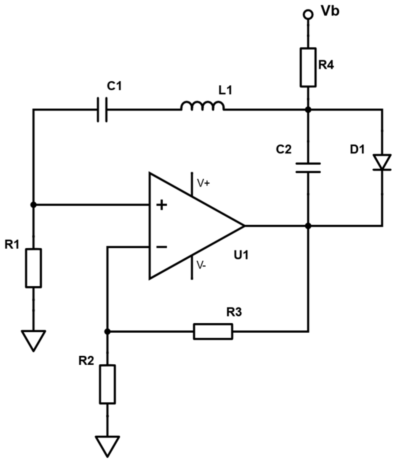
2. Vilnius Oscillator Model

The schematic of the Vilnius chaotic oscillator is depicted in Figure 1. The circuit is easy to implement and modify, as it includes no unique components, just the off-the-shelf operational amplifier, diode, capacitors, inductors, and resistors.

This oscillator exhibits complex behavior under specific component parameters despite being relatively simple. The frequency of the waveforms observed in the circuit is determined by reactive components C₁, L₁, and C₂. Thus, it is possible to adapt the scheme for the frequency range of interest. Diode D₁ is the mandatory nonlinear element needed for the chaotic oscillator. It can be a general-purpose silicon diode such as 1N4148 or Schottky diode. Moreover, no special requirements apply to the operational amplifier. A reader can use, for example, an LTspice computer simulation program to obtain a quick insight into the circuit’s operation and observe typical waveforms. However, even such a brief study reveals that the number of parameters that affect the system’s dynamics is too large to adopt a trial-and-error approach when the robust chaos is of interest. That is why the study of nonlinear dynamics using bifurcation diagrams must be performed to identify the regions of chaotic behavior for further practical implementation of the Vilnius oscillator.

In this study, a system of equations initially developed in [15] is used to describe the dynamics of the oscillator:

$$\frac{dx}{dt}=y,$$

(1)

$$\frac{dy}{dt}=ay-x-z,$$

(2)

$$\epsilon \frac{dz}{dt}=b+y-c(e^z-1),$$

(3)

where the dimensionless variables and parameters suggested for conventional numerical analysis are:

$$x=\frac{V_{C1}·q}{k_B·T};\hspace{1em}y=\frac{I_{L1}·q·\sqrt{\frac{L}{C_1}}}{k_B·T};\hspace{1em}z=\frac{V_{C2}·q}{k_B·T},$$

(4)

$$a=\frac{\left(k-1\right)·R_1}{\sqrt{\frac{L}{C_1}}};\hspace{1em}b=\frac{I_{R4}·q\sqrt{\frac{L}{C_1}}}{k_B·T};\hspace{1em}c=\frac{I_S·q·\sqrt{\frac{L}{C_1}}}{k_B·T};\hspace{1em}\epsilon =\frac{C_2}{C_1}.$$

(5)

To express the current through R₄, it is assumed that R₄ >> R_1, so according to Ohm’s law:

$$I_{R4}=\frac{V_b}{R_4}.$$

(6)

The gain of the non-inverting amplifier is expressed as:

$$k=1+\frac{R_3}{R_2}.$$

(7)

k_B is Boltzmann’s constant; T is the temperature in Kelvins; q is the electron charge.

The system’s parameters of interest are a, b, and ε, which could be adjusted by input voltage, variable capacitor C₂, and variable resistors R₁, R₂, R₃, and R₄.

The study of the nonlinear dynamics of the Vilnius oscillator will be provided based on one and two-parameter bifurcation diagrams that allow estimation of the system’s mode of operation for various combinations of component values. However, this approach requires obtaining the discrete-time model of the original oscillator. The models could be constructed by application of the Poincaré map. In the case of the Vilnius oscillator, y = 0 is selected as the Poincaré plane. Thus, the trajectories crossing this plane from one side will define the sampled model and provide the required information on the periodicity of the regimes under study, see Figure 2.

All the calculations are made utilizing specially prepared MATLAB scripts, including the solution of the equations with the Runge–Kutta (4,5) method, implemented in the ode45 function. As constructing bifurcation maps and complete bifurcation diagrams in the wide range of system parameters is time-consuming, the Parallel Computing Toolbox functionality has been intensively utilized to efficiently distribute the computation tasks between all available physical cores of the computer. The scripts are prepared to be very flexible and reusable, allowing for analysis of any well-defined system by accepting system models as function variables, all analysis parameters can be specified, and additional scripts are provided for result refinement to shorten the feedback loop. Both brute-force and MCBG scripts are applied at various stages of the analysis. While the brute-force scripts iteratively solve for the system’s next points in a given axis to generate bifurcation maps and diagrams, the MCBG scripts compute the fixed points of a system using the Newton–Raphson iteration and define their stability estimating the multipliers of the obtained Jacobian matrixes, along with a host of other algorithms and filters to generate period specific bifurcation branches which are combined to form complete bifurcation diagrams. The results of the numerical calculations and the analysis of the obtained diagrams are provided in the next section.

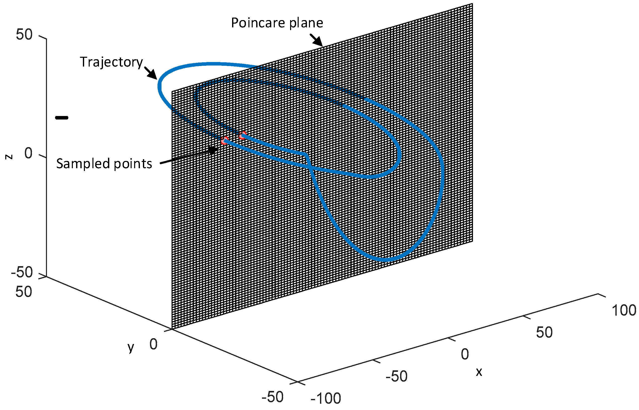
3. Complete Bifurcation Analysis

The main goal of the current research is to study the dynamics of the Vilnius oscillator, operating in the parameter range viable for applications in wireless sensor networks. The parameters under study are b- defined by the voltage V_b, a- related to the amplifier gain k, and ε- defined by C₁ and C₂. The task is to provide the study of complex phenomena observed in the chaotic oscillator at different combinations of selected defined parameters.

In the following subsections, the study of nonlinear dynamics of the oscillator is based on the construction of two-parameter bifurcation diagrams (bifurcation maps) and the complete bifurcation analysis of the corresponding one-parameter diagrams as the cross-sections of the map.

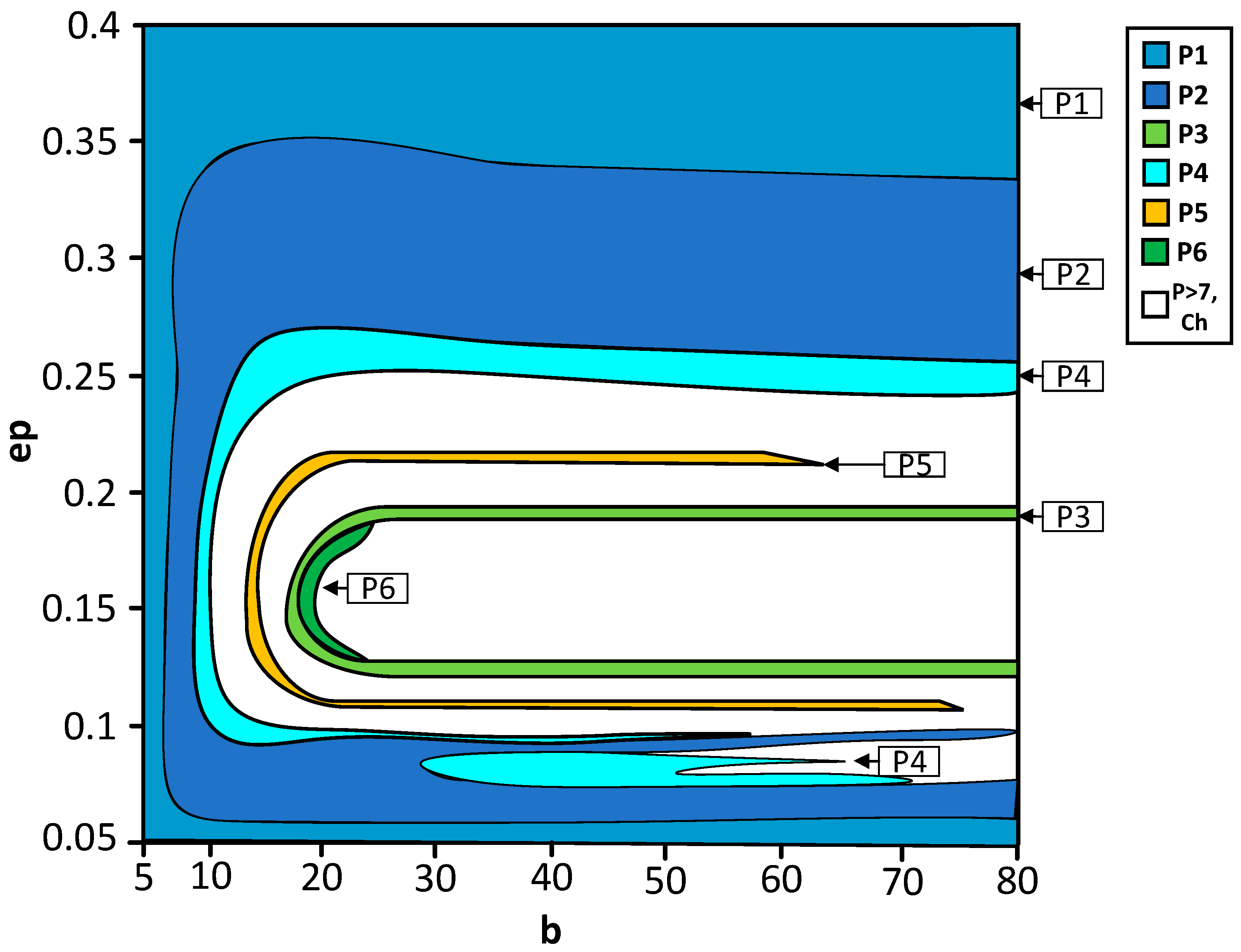
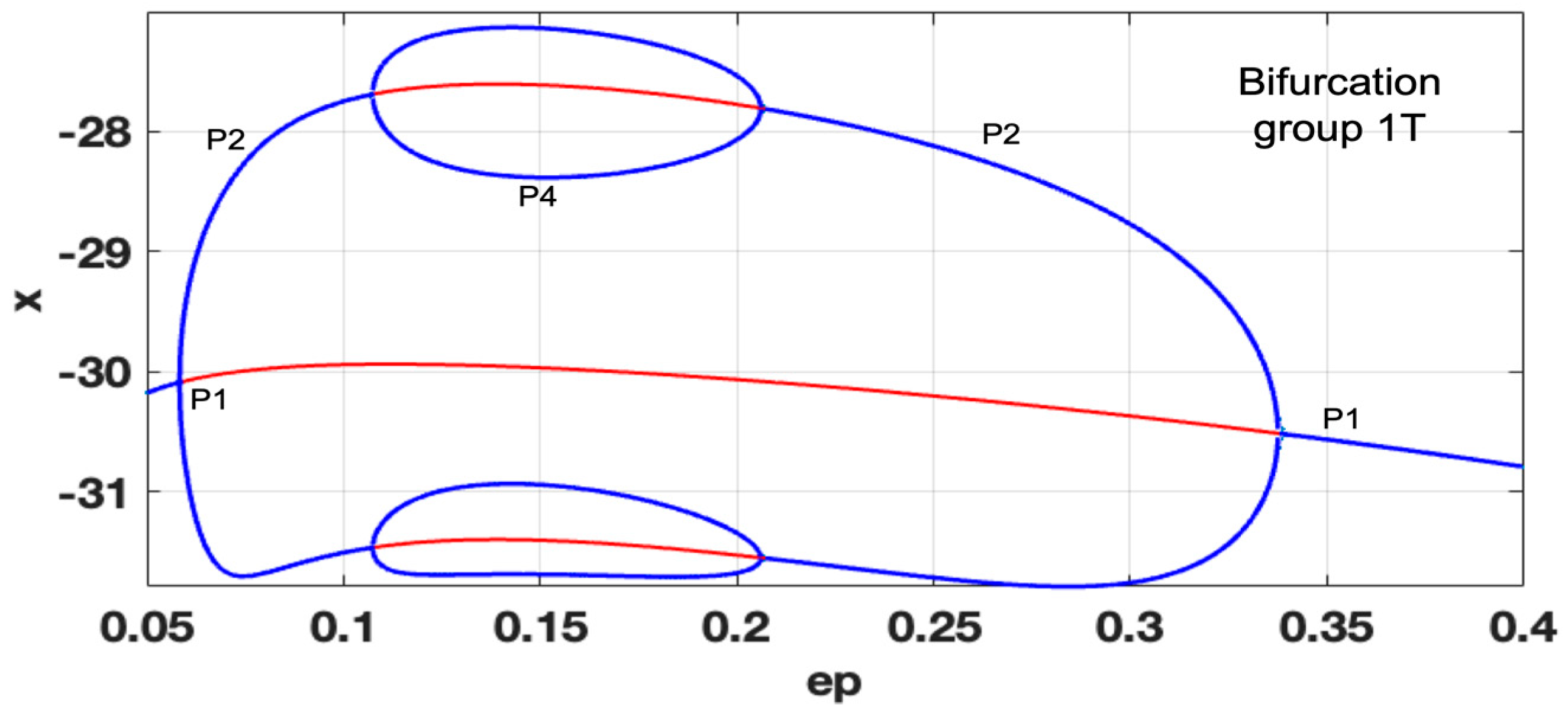
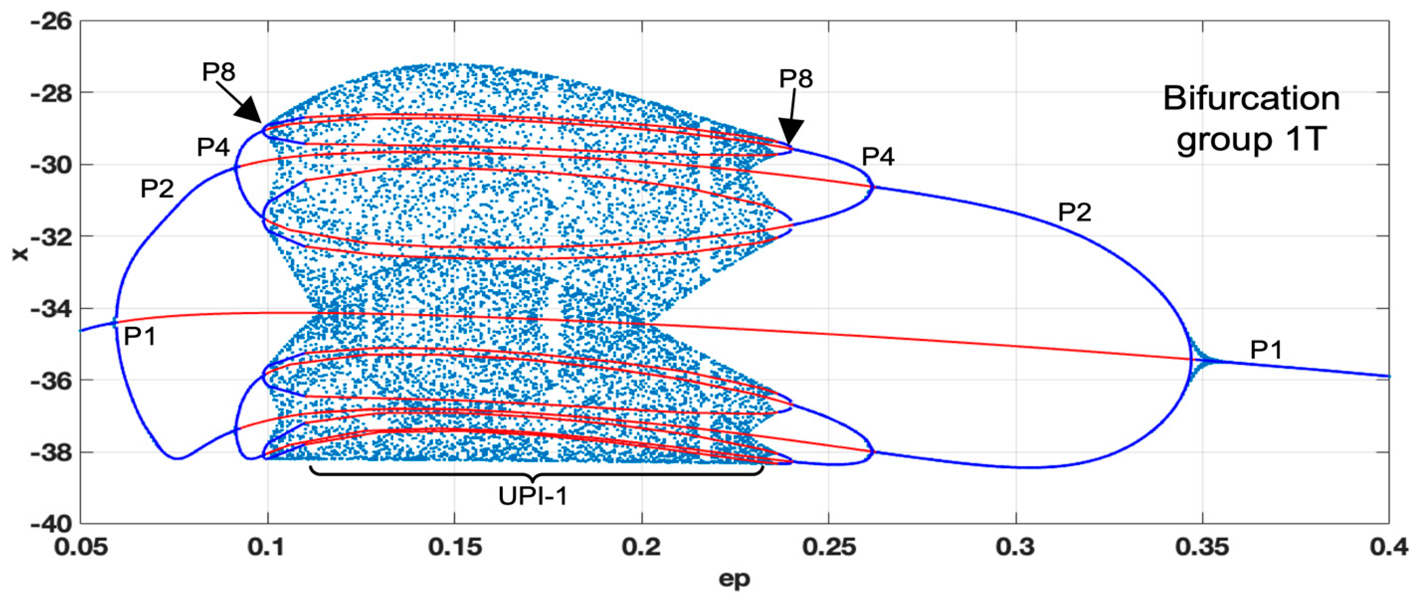
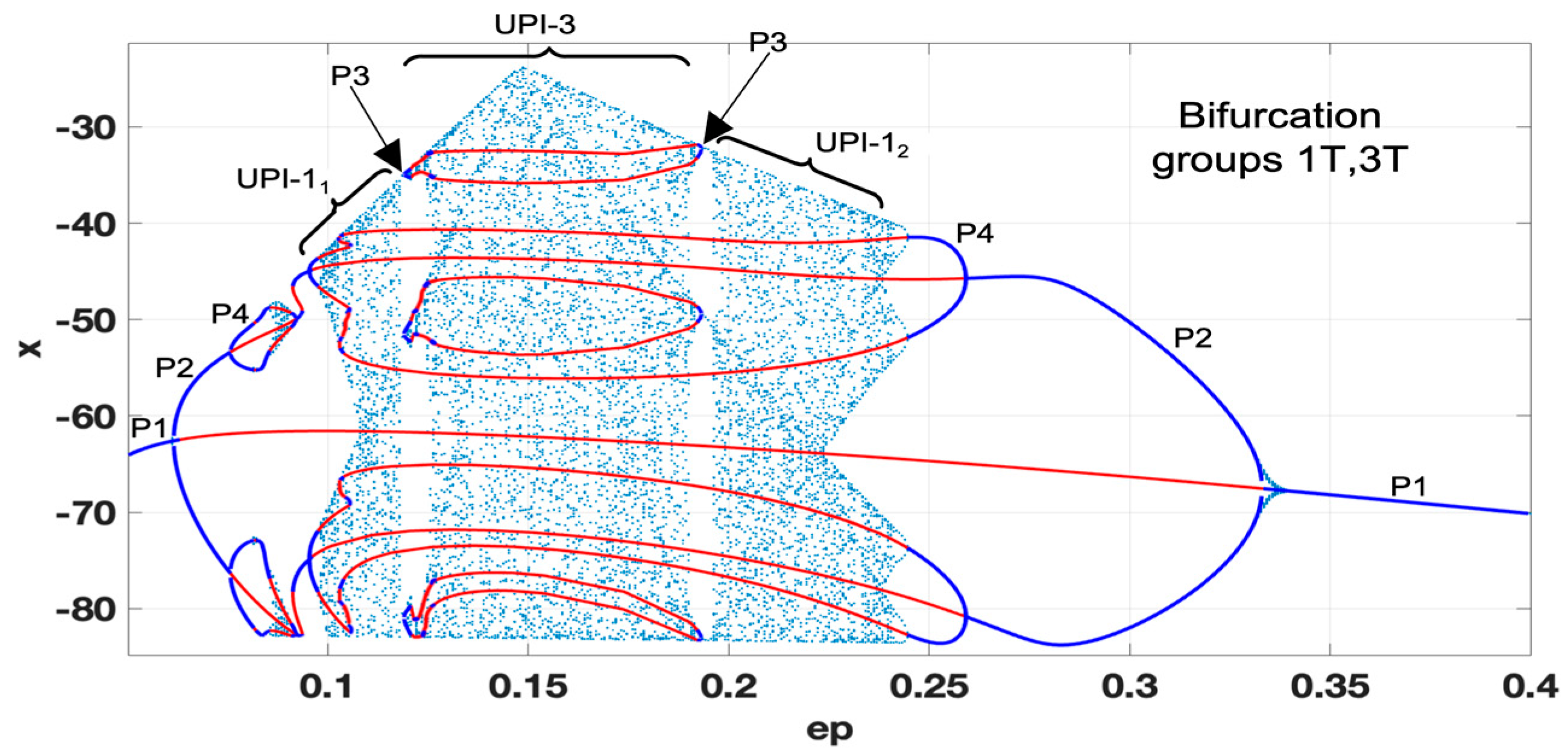
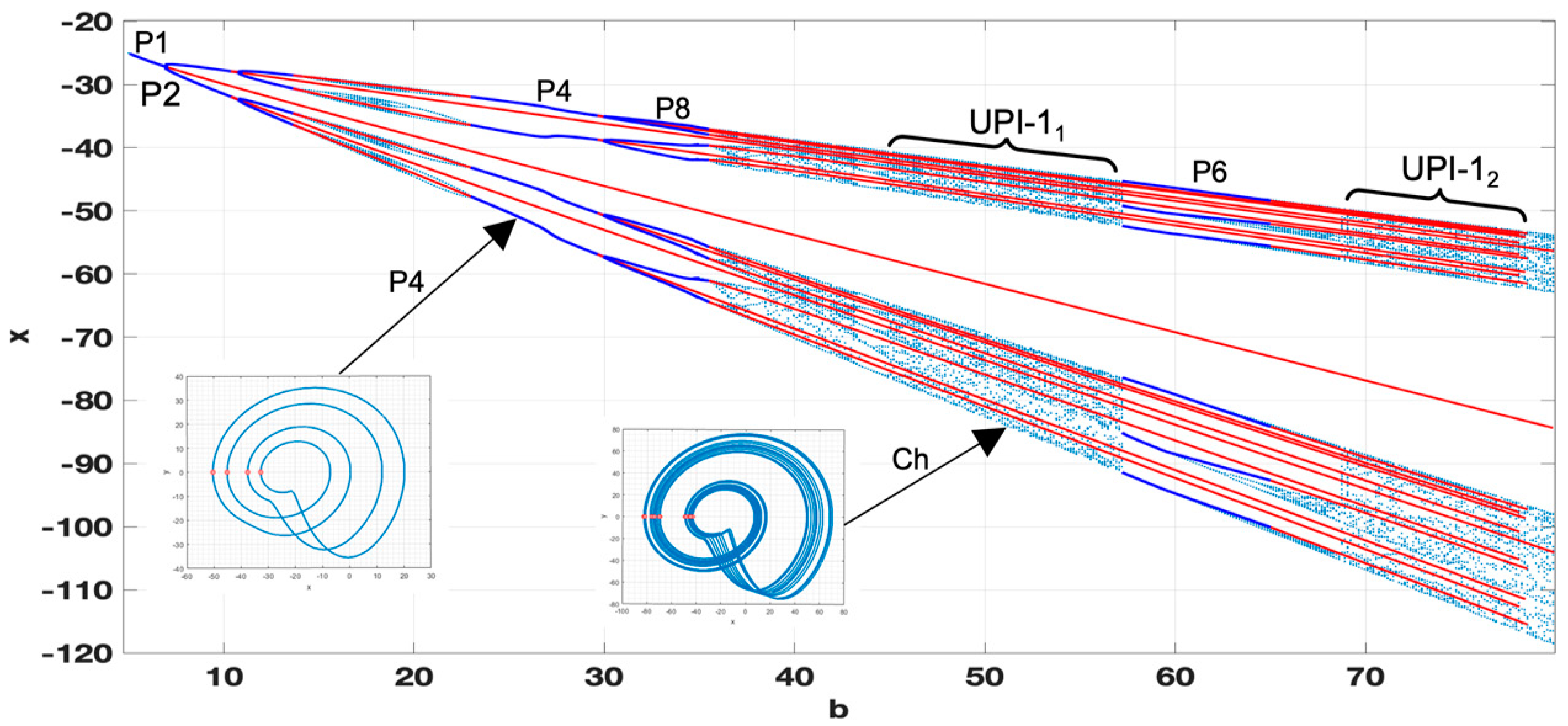
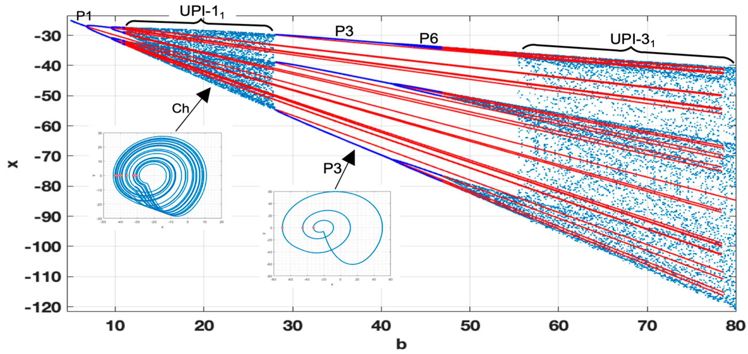
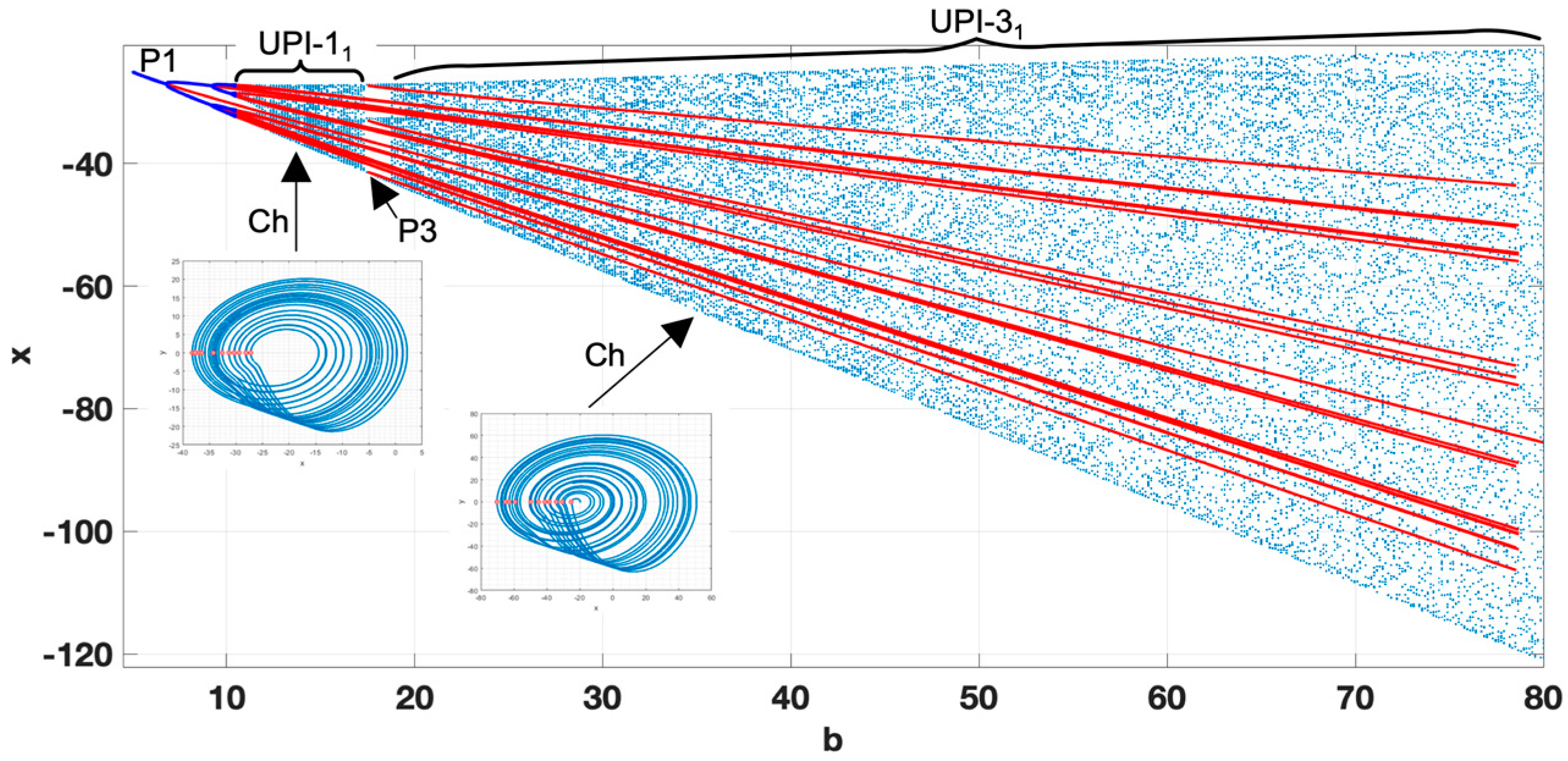
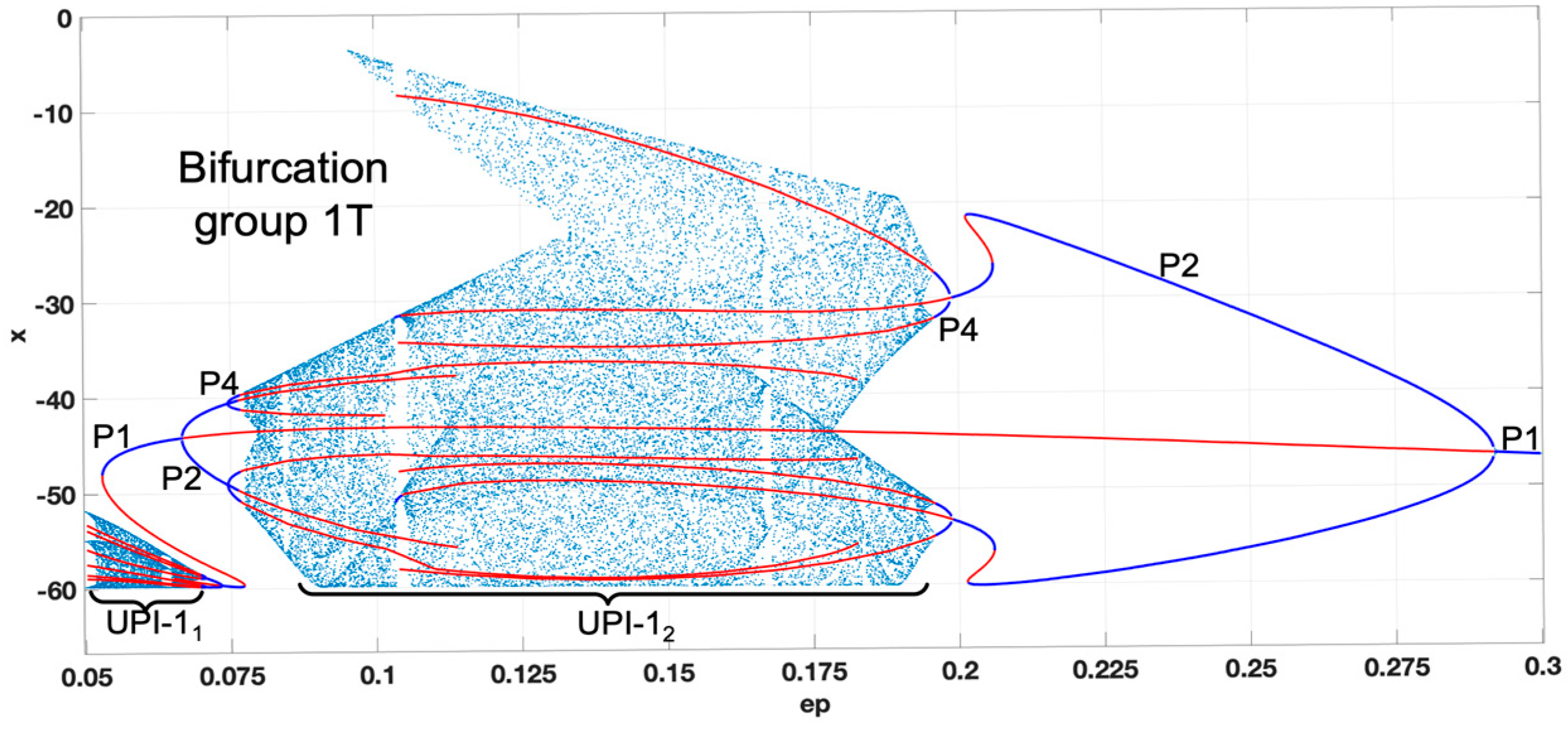
3.1. Dynamics of the Oscillator in the b-ε Plane

First, the parameter a is fixed at the value 0.3, and the system’s dynamics are studied, varying b and ε. The obtained map for ε = 0.05–0.4 and b = 5–80 is shown in Figure 3. Periodic operation modes are depicted with different colors up to period-6, and other high-periodic regimes and chaos are shown as white regions.

The bifurcation map demonstrates that for low values of b (defined by the input voltage), the system’s dynamics are mainly periodic—exhibiting P1 to P4 oscillations for all values of ε. For example, for b = 5, the P1 motion is the only possible operation regime independent of the ε. For b = 7, the system exhibits P1-P2-P1 transition, returning to the stable P1 mode for larger values of ε. From a practical point of view, the system could not be used as the generator of chaotic oscillations for low voltages (defined by b < 12). This is also illustrated in Figure 4, where stable regimes are depicted in blue and unstable ones in red. The complete bifurcation diagram shows the clear transition from P1 to P4 and back to P1 through subsequent forward and reverse period doublings without any signs of UPIs, defining the chaotic oscillations. The construction of the unstable branches allows the verification that all the regimes represent a single bifurcation group 1T. No coexisting chaotic attractors are detected either. Thus, operating the Vilnius oscillator in a very low-voltage mode, giving the benefits of high energy efficiency, would not provide the required chaotic signals.

However, there is a definite border (b > 12), where the system becomes chaotic for a relatively wide range of ε values. There could be intermittent chaotic dynamics (with various periodic windows) or robust chaos without interrupting periodic modes. Figure 5 shows a classical period-doubling route to chaos enclosing the interval with UPI₁, where only unstable regimes are observed, and the chaotic oscillations could be assumed robust. It can be inferred that setting system parameters within the range ε = 0.1–0.23 should guarantee stable chaotic oscillations without the issue of transitioning to some periodic mode due to external noise or fluctuations in the component’s values. At the same time, the bifurcations map shows that minor variations of b could lead to the transition to P5 mode on the right or P4 operating regime on the left.

The system’s behavior remains similar for higher values of b, as shown in Figure 6. However, the amplitude of x (related to V_C1) increases. Compared to the previous diagram, the system exhibits a non-smooth transition to chaos from the left side. This phenomenon could be explained by a diode in the circuit, defining the non-smooth switchings as the voltage rises and a certain threshold is reached. It has been noticed that the systems with non-smooth bifurcations could exhibit robust chaotic oscillations. However, in this case, we observe the appearance of the separate UPI-1₁, UPI-3, and UPI-1₂, corresponding to the robust chaotic regions. Periodic windows in the chaotic regions appear, forming narrow regions of the P3 modes. The transition to stable periodic regimes is observed as ε > 0.24. In practice, the utilization of UPI-3 and UPI-1₂ modes is more advisable, providing a wider range of ε values that ensure robust chaos. Figure 3 also shows that for these modes, the fluctuations of the b would not cause the transitions to any periodic windows.

The second part of the investigation in the b-ε plane is dedicated to constructing the complete bifurcation diagrams for fixed values of ε and varying the parameter b. For ε < 0.12, a wide diversity of dynamical patterns could be observed, as b is varied. Figure 7 shows period doublings, intermittent chaos and wide periodic windows. These regimes could not be relevant for practical applications, as any slight supply voltage variations could cause unpredicted transitions between different modes, compromising the whole system’s security. Chaotic attractors observed in the corresponding regions, as the Ch attractor in Figure 7, are not dense enough, indicating insufficient diversity required by practical communication systems.

However, the further increase in parameter ε leads to the formation of several robust chaotic regions, such as UPI-1₁ and UPI-3₁ shown in Figure 8, with acceptable characteristics and durability to parameter changes. All large periodic windows converge to a single wide P3-P6 window, as seen in Figure 8. In practice, we are interested in the low-voltage operation of the system, so the region of b = 12–28, corresponding to the UPI-1₁, formed as a result of the period-doubling cascade within the 1T bifurcation group, is the most appropriate for the generation of robust chaotic oscillations.

Setting the ε = 0.15 in the middle of the predicted chaotic region in the bifurcation map, as seen in Figure 3, it is possible to obtain the diagram where all periodic windows shrink to a negligible stable P3 mode, and the continuous robust chaotic area (UPI-3₁) is formed. This is demonstrated in Figure 9. The advisable region to operate the oscillator would be in the range of b = 20–80.

As it can be deduced from Figure 3, the further increase in ε leads to the deterioration of chaotic dynamics and diagrams, such as those shown in Figure 7 and Figure 8, could be obtained.

In the following subsection, we choose the lowest possible value of b (directly connected to the input voltage), which ensures robust chaotic oscillations and provide the complete bifurcation analysis, as ε and a are varied.

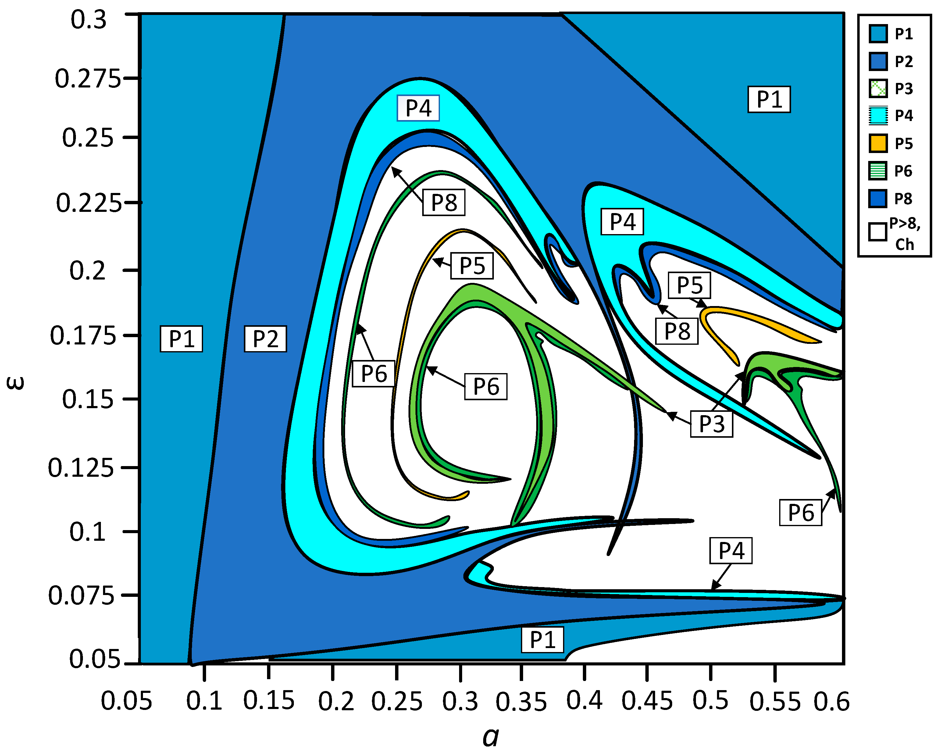
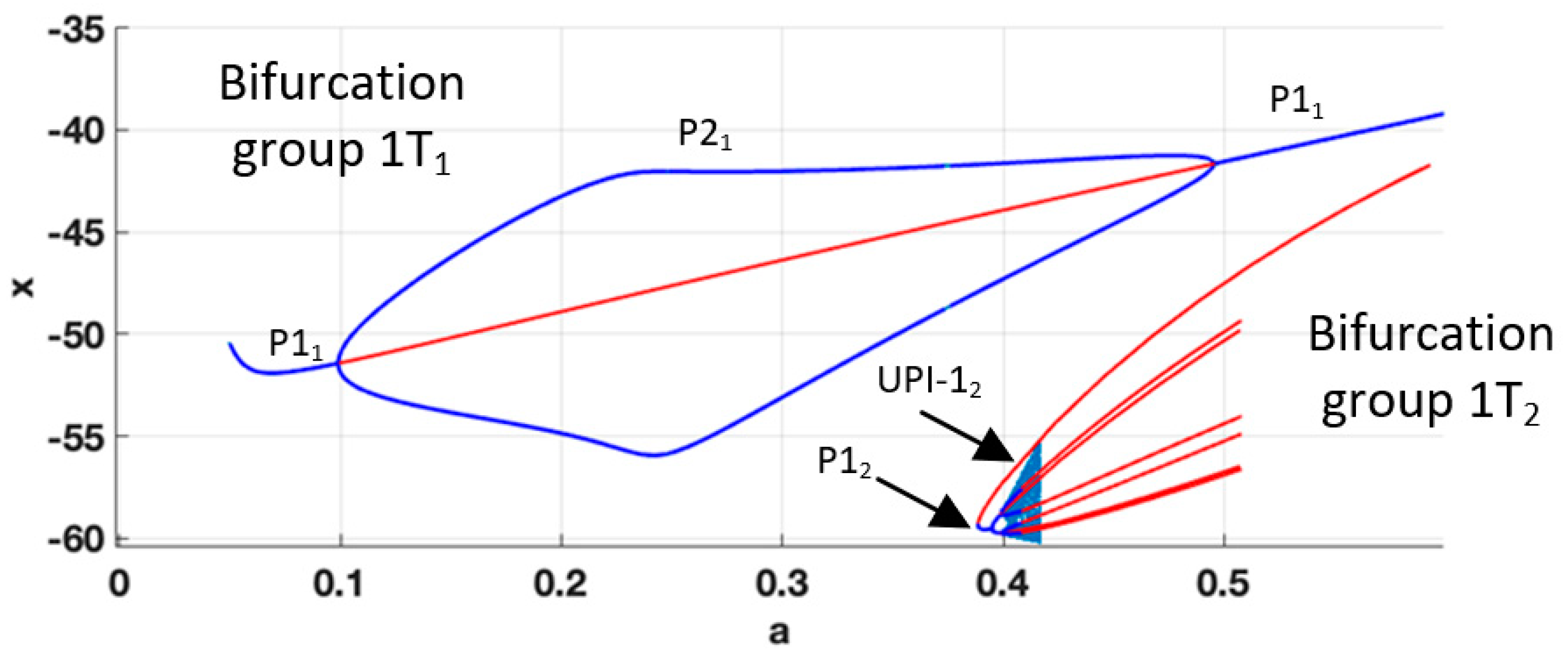
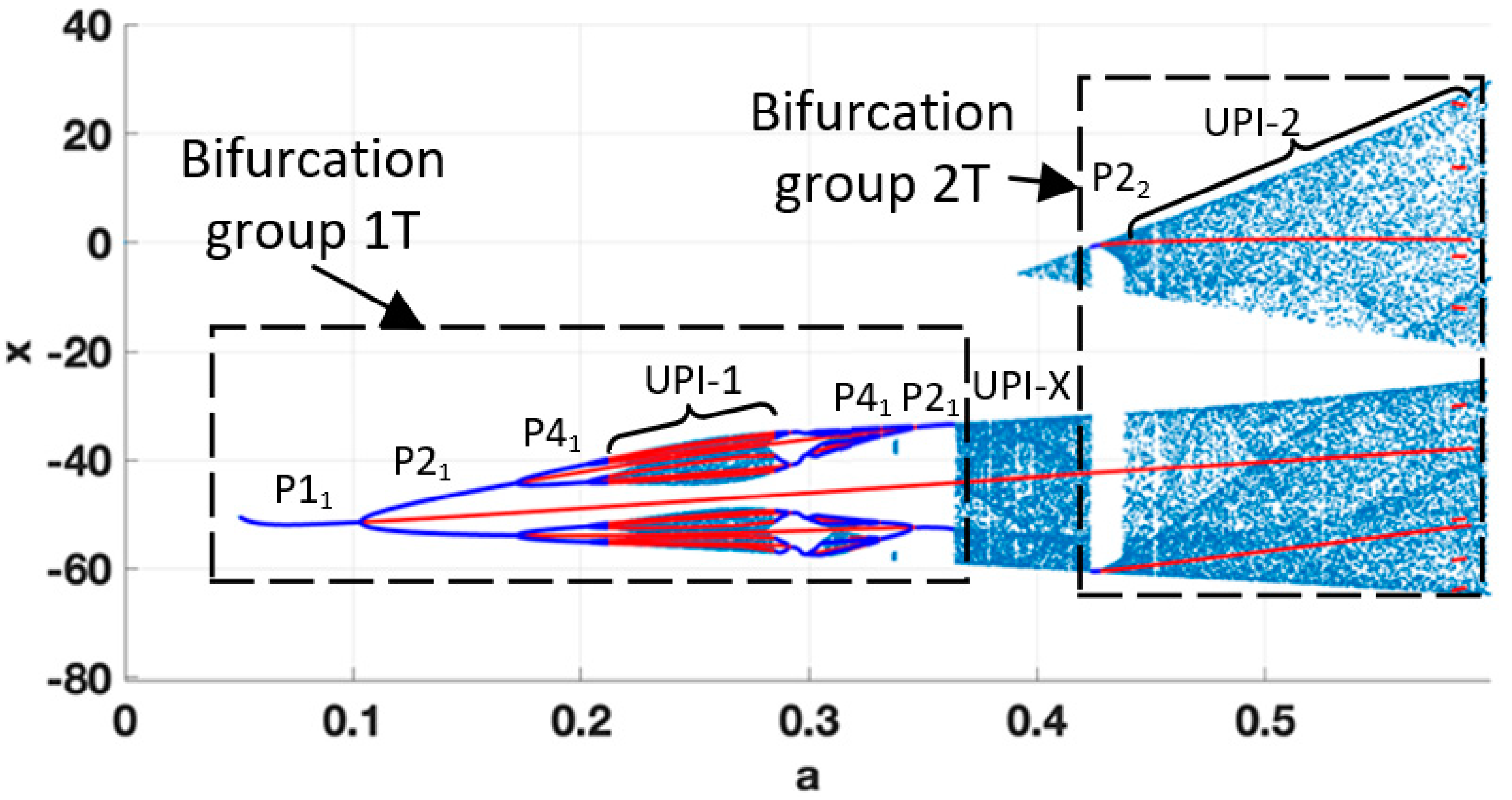
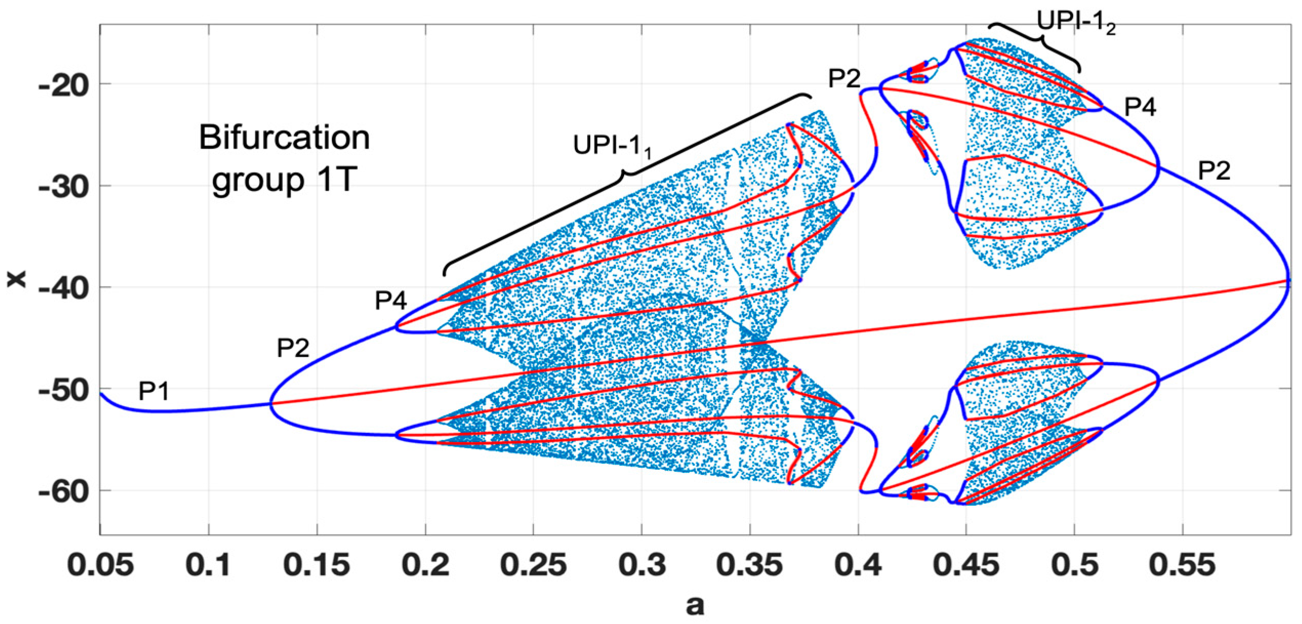
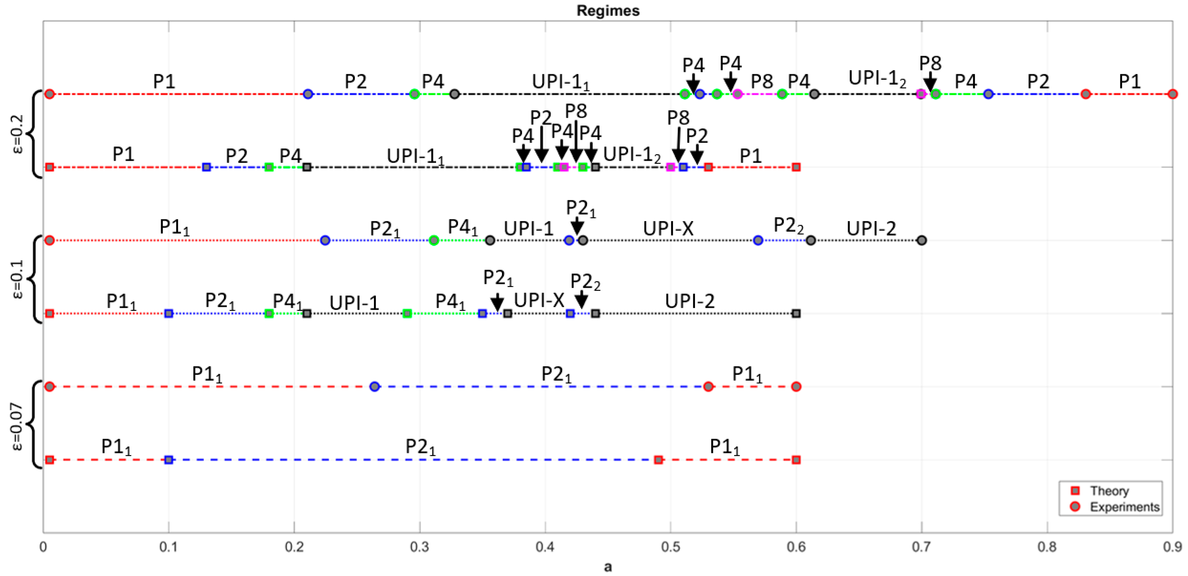
3.2. Dynamics of the Oscillator in the a-ε Plane

The first step is the construction of the bifurcation map, selecting ε and a as primary and secondary bifurcation parameters. The obtained two-parameter bifurcation map, depicting periodic regimes up to P8 and chaos (white regions), is shown in Figure 10.

The diagram shows the complex distribution of periodic and chaotic regions in the selected parameter space, including some unusual “spiking patterns” previously observed in other systems and described by Jason Gallas, e.g., in [24]. The map allows for preliminary conclusions on the regions of possible practical interest. For a < 0.21, only P1-P8 regimes are observed without any transitions to chaos in the whole range of ε values. As a increases, more complex transitions between periodic modes and chaos could be observed for different values of ε. It should be noticed that the bifurcation map is obtained employing brute-force iterations and, thus, sometimes, does not reveal the actual structure of the bifurcation patterns. Therefore, it is necessary to construct the complete bifurcation diagrams as the “cross-sections” of the obtained map. Construction of the periodic skeletons and branch continuation techniques allow the detection of all stable and unstable regimes in the parameter range of interest.

First, we obtain the complete bifurcation diagram for ε = 0.07. The map in Figure 10 shows that the transition P1-P2-P1 should be observed. However, the complete bifurcation diagram in Figure 11 shows two coexisting bifurcation groups—1T₁ and 1T₂. 1T₁ is formed by the predicted P1₁-P2₁-P2₁ cascade. However, 1T₂ coexists with 1T₁, becoming stable for a = 0.385 and experiencing the full period-doubling cascade with the formation of UPI-1₂, indicating chaotic dynamics. The chaotic attractor collides with the unstable branch of P1₂ at a = 0.415 and is no longer observed. The appearance of two coexisting bifurcation groups with stable regimes could lead to unpredicted “jumps” from stable P2 to chaotic motion due to the inevitable presence of noises in the real circuit. Thus, the use of the detected chaotic regime is not a viable option.

As the value of ε = 0.1, the complete bifurcation diagram reveals the appearance of non-smooth phenomena, manifesting as abrupt changes in the system’s dynamics shown in Figure 12. The diagram is formed by bifurcation groups 1T and 2T. The first group shows the transition to UPI-1 through the period-doubling cascade and further reverse transition up to P2₁. However, for a = 0.36, the non-smooth transition to UPI-X is observed, and the system exhibits robust chaos. The bifurcation group 2T is composed of a narrow region of P2₂ regime with further rapid chaotization (see UPI-2). For the observed parameters, the recommended values of a, ensuring robust chaotic oscillations, not affected by small perturbations, could be a = 0.25, 0.4, 0.5, pointing to the middle parts of the UPIs.

Figure 13 is the next diagram obtained for ε = 0.2, and it shows a single bifurcation group 1T with a complex structure of transitions from P1 to UPI-1₁, then to P2 with double-sided period-doubling cascade, finally leading to the formation of another UPI-1₂, and reverse transition to P2 mode of operation. The observed transitions are smooth; the UPI regions do not include significant periodic windows and could be used as regions of robust chaos.

The last bifurcation diagram is obtained by fixing the value of a = 0.4 and selecting ε as the bifurcation parameter, as shown in Figure 14. If we start from ε = 0.3 and decrease the value, we observe the period-doubling route to robust chaos (UPI-1₂). The manifestation of the non-smooth nature of the systems leads to the sudden transitions and disappearance of chaotic attractor for ε = 0.06. The UPI-1₁, observed for the values of ε = 0.01–0.06, coexists with the stable P1 regimes and could not be used as a reliable source of chaotic oscillations, leaving the UPI-1₂ as the only viable option.

4. Experimental Verification

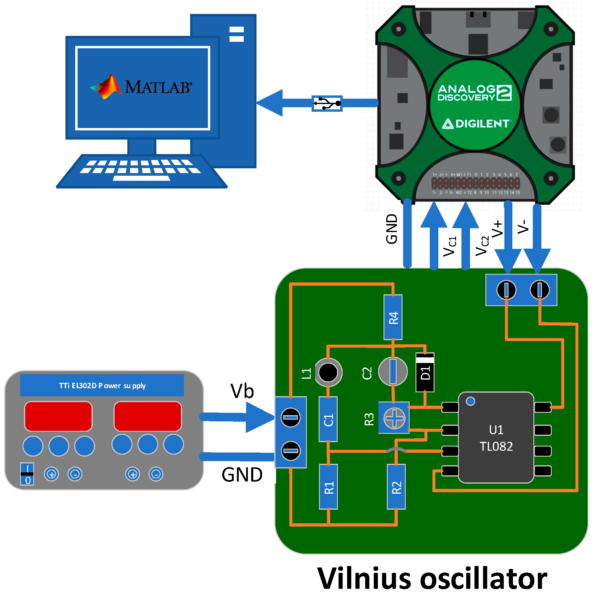
This section includes a description of the experimentally obtained results. The most complex diagrams were verified, obtaining the phase portraits and allowing the regime’s periodicity detection. First, we provide a short description of a simple experimental setup. Further, the analysis and compilation of the obtained results are provided.

4.1. Test Setup

The experimental setup is shown in Figure 15. The Vilnius oscillator is designed from off-the-shelf components, including: operational amplifier U₁—TL082, diode D₁—1N4148, R₁ = 1 kΩ, R₂ = 10 kΩ, R₄ = 20 kΩ, R₃ = 10 kΩ (variable), L₁ = 1 mH, C₁ = 1 nF, C₂ = 1 nF (variable). The TTi EL302D power supply provides the input voltage V_b.

Analog Discovery 2 is used as a universal tool to power the U₁ with ±5 V and capture the voltages on C₁ and C₂. Further, the data are transferred to the Digilent WaveForms application and saved for processing in Matlab R2023a. The experimental setup allows variations of R₃, C₂, and V_b, that are directly connected to the a, ε, and b parameters of the Vilnius oscillator (see Equations (4)–(7)). To reduce the confusion and compare experimental results to the numerically obtained diagrams, the values of a, ε, and b will be used in all the graphs.

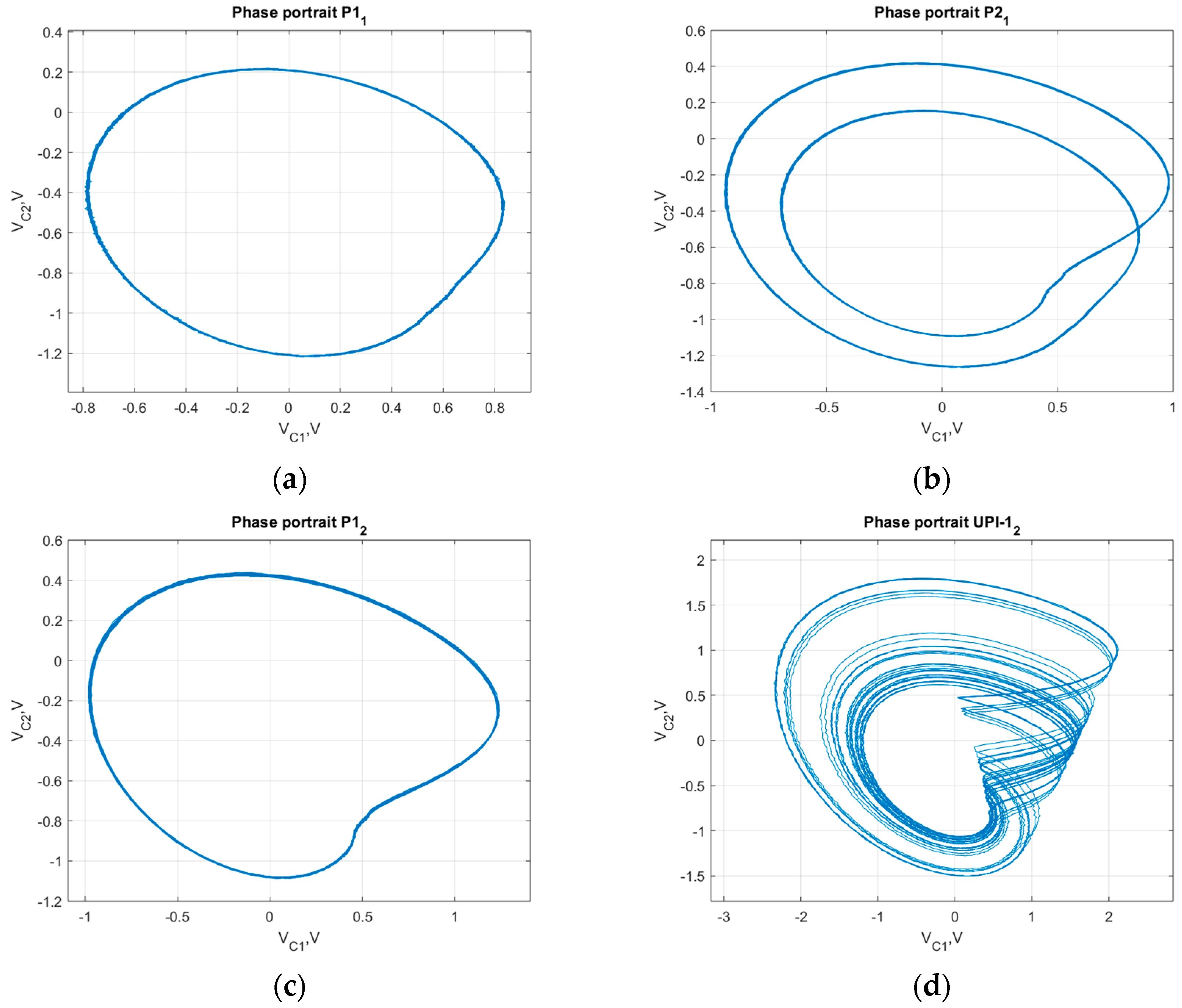
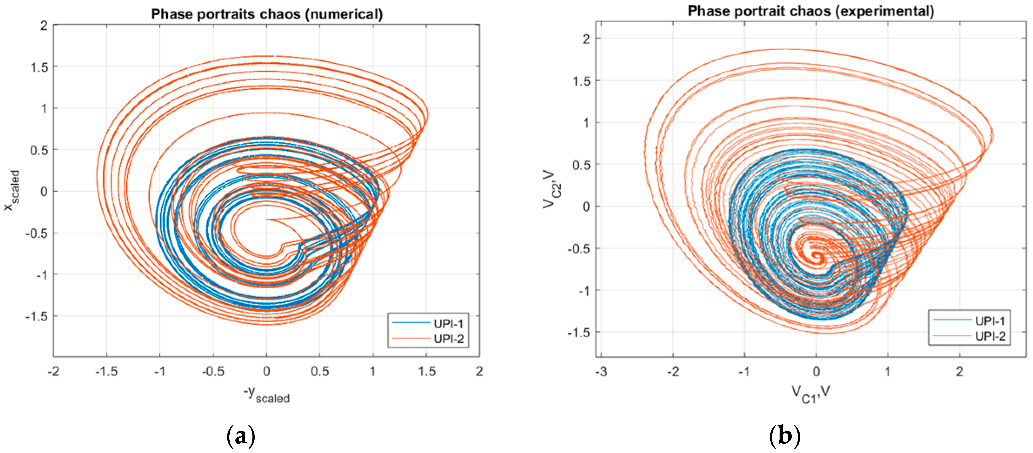
4.2. Experimental Results and Analysis

We start with the verification of selected diagrams obtained in Section 3.2 where b = 30 is fixed, and parameters ε and a are varied (adjusting C₂ and R₃), as the proposed diagrams provide the most complicated structures that would allow us to evaluate the degree of accuracy of the obtained numerical results. The simplest way to verify the validity of theoretical results is to obtain the waveforms and appropriate phase portraits for selected points in the parameter space, also marking the bifurcation points. Taking the complete bifurcation diagram from Figure 11 as the basis, we capture the phase portraits for different modes, as b = 30, ε = 0.07, and a varied from 0.05 to 0.6—see Figure 16.

As in Figure 11, the phase portraits show the transition P1-P2-P1 as the value a is increased through the range. The appearance of coexisting chaotic mode was also identified experimentally. Practically, the P1₂ was not “stable” as transient jumps to chaotic mode were observed—the corresponding chaotic attractor is shown in Figure 16d. The jumps were caused by the noise present in the circuit, and even movement of the connecting wires could cause the system to go to/from chaotic mode.

These observations allow us to conclude that the MCBG gives reliable information about the predicted modes of operation of the circuit. However, it is impractical to provide phase portraits for every single regime. Still, it would be more beneficial to aggregate the information for experimentally observed modes and points of transitions in a single graph. For that purpose, we propose using a mode-transition graph—providing data on the ranges for all regimes and depicting transition points. This analogue of the bifurcation diagram also allows the comparison of experimentally and numerically obtained results. The graph presented in Figure 17 summarizes the data from the bifurcation diagrams, shown in Figure 11, Figure 12 and Figure 13, and experimental results.

The obtained mode-transition graphs clearly show that it was possible to verify theoretically obtained results successfully. For each ε value, the pair or graphs show that the sequences of transitions between periodic and chaotic modes of operation remain the same. This is true for relatively simple cases—e.g., for ε = 0.07, where the P1-P2-P1 transition is observed, and also for highly complex mode transition structures with multiple forward and reverse period-doubling cascades and chaotization scenarios—e.g., for ε = 0.1 and ε = 0.2. It should be mentioned that despite the direct correspondence of the mode transition sequences, the practically obtained ranges of parameter values for each mode differ. One commonly observed pattern is that in experiments, P1 mode loses its stability for higher values of a, leading to the general shift of the mode transition graph and corresponding transition (bifurcation) points. The observed mismatches could be explained by experimental component tolerances, parasitic elements, and unavoidable noises in the practically implemented circuit.

It should be noted that the phase portraits could still be used to identify some specific features of the regimes under interest. For example, for ε = 0.1, both UPI-1 and UPI-2 define the appearance of the chaotic modes of operation shown in Figure 17. However, the strange attractors of these regimes differ in the density of orbits and amplitude, which could be of particular interest when applying the obtained signals to actual data security circuitry. Figure 18 compares two chaotic attractors for a = 0.25 (UPI-1) and a = 0.5 (UPI-2), obtained numerically (scaled for the comparison) and experimentally.

The similarity of theoretical and experimental attractors highlights the validity of numerically obtained results and the applicability of the MCBG for the prediction, analysis, and characterization of complex dynamics of nonlinear systems.

5. Conclusions

The growing number of applications of chaotic systems requires the more complete analysis of the nonlinear dynamics of chaos generators. The paper demonstrated the numerical study and experimental results on possible chaotization scenarios and various nonlinear phenomena observed in the Vilnius chaotic oscillator as system parameters vary. It has been shown that constructing the bifurcation maps allows for the convenient identification of the most appropriate parameter ranges for obtaining robust chaotic modes of operation. The consequent construction of complete bifurcation diagrams and application of the MCBG allows for in-depth analysis of transitions between different modes of operation. It identifies the non-smooth phenomena and coexisting attractors that could not be detected by the bifurcation maps. It has been shown that the robust chaotic modes could be obtained, but only for higher values of operating voltages. Thus, low-power operation of the Vilnius oscillator is not feasible. The ability to generate chaotic attractors with different amplitudes and orbit densities highlights the trade-off between energy efficiency and increased level of security.

Nevertheless, the experimental verification allowed the conclusion that numerical results qualitatively match the experimental ones, providing the same sequence of bifurcations and periodic or chaotic regimes, the presence of parasitic elements, limited tolerances of the components, and noises lead to the mismatch in the parameter values, where the transitions between the modes occur. Future work will focus on modifying the existing models, including the parasitic parameters of the oscillators, to find the causes of the mismatch of the bifurcation points. The laboratory experiments will be provided to obtain the relevant data on the tradeoff between the energy efficiency of Vilnius oscillators, robustness of generated chaos, and potential security levels ensured, defining the guidelines for selecting the chaotic modes according to the requirements determined by specific applications.

References

1. Litvinenko, A.; Aboltins, A. Chaos Based Linear Precoding for OFDM. In Proceedings of the 2015 Advances in Wireless and Optical Communications (RTUWO), Riga, Latvia, 5–6 November 2015; pp. 13–17. [Google Scholar]
2. Litvinenko, A.; Bekeris, E. Probability Distribution of Multiple-Access Interference in Chaotic Spreading Codes Based on DS-CDMA Communication System. Elektronika ir Elektrotechnika 2012, 123, 87–90. [Google Scholar] [CrossRef] [Green Version]
3. Babajans, R.; Cirjulina, D.; Grizans, J.; Aboltins, A.; Pikulins, D.; Zeltins, M.; Litvinenko, A. Impact of the Chaotic Synchronization’s Stability on the Performance of QCPSK Communication System. Electronics 2021, 10, 640. [Google Scholar] [CrossRef]
4. Dantas, W.G.; Rodrigues, L.R.; Ujevic, S.; Gusso, A. Using Nanoresonators with Robust Chaos as Hardware Random Number Generators. Chaos 2020, 30, 043126. [Google Scholar] [CrossRef] [PubMed]
5. Yu, F.; Li, L.; Tang, Q.; Cai, S.; Song, Y.; Xu, Q. A Survey on True Random Number Generators Based on Chaos. Discret. Dyn. Nat. Soc. 2019, 2019, 2545123. [Google Scholar] [CrossRef]
6. Majumder, B.; Hasan, S.; Uddin, M.; Rose, G.S. Chaos Computing for Mitigating Side Channel Attack. In Proceedings of the 2018 IEEE International Symposium on Hardware Oriented Security and Trust (HOST), Washington, DC, USA, 30 April 2018–4 May 2018; pp. 143–146. [Google Scholar]
7. García-Grimaldo, C.; Bermudez-Marquez, C.F.; Tlelo-Cuautle, E.; Campos-Cantón, E. FPGA Implementation of a Chaotic Map with No Fixed Point. Electronics 2023, 12, 444. [Google Scholar] [CrossRef]
8. Capligins, F.; Litvinenko, A.; Kolosovs, D.; Terauds, M.; Zeltins, M.; Pikulins, D. FPGA-Based Antipodal Chaotic Shift Keying Communication System. Electronics 2022, 11, 1870. [Google Scholar] [CrossRef]
9. Petrzela, J. Chaos in Analog Electronic Circuits: Comprehensive Review, Solved Problems, Open Topics and Small Example. Mathematics 2022, 10, 4108. [Google Scholar] [CrossRef]
10. Chen, H.; Chen, P.; Wang, S.; Lai, S.; Chen, R. Reference-Modulated PI-DCSK. A New Efficient Chaotic Permutation Index Modulation Scheme. IEEE Trans. Veh. Technol. 2022, 71, 9663–9673. [Google Scholar] [CrossRef]
11. Paul, P.S.; Dhungel, A.; Sadia, M.; Hossain, R.; Hasan, S. Self-Parameterized Chaotic Map for Low-Cost Robust Chaos. J. Low Power Electron. Appl. 2023, 13, 18. [Google Scholar] [CrossRef]
12. Aboltins, A.; Tihomorskis, N. Software-Defined Radio Implementation and Performance Evaluation of Frequency-Modulated Antipodal Chaos Shift Keying Communication System. Electronics 2023, 12, 1240. [Google Scholar] [CrossRef]
13. Karimov, T.I.; Druzhina, O.S.; Ostrovskii, V.Y.; Karimov, A.I.; Butusov, D.N. The Study on Multiparametric Sensitivity of Chaotic Oscillators. In Proceedings of the 2020 IEEE Conference of Russian Young Researchers in Electrical and Electronic Engineering (EIConRus), St. Petersburg/Moscow, Russia, 27–30 January 2020; pp. 134–137. [Google Scholar]
14. Azar, A.T.; Serranot, F.E.; Vaidyanathan, S. Chapter 10—Sliding Mode Stabilization and Synchronization of Fractional Order Complex Chaotic and Hyperchaotic Systems. In Mathematical Techniques of Fractional Order Systems; Azar, A.T., Radwan, A.G., Vaidyanathan, S., Eds.; Advances in Nonlinear Dynamics and Chaos (ANDC); Elsevier: Amsterdam, The Netherlands, 2018; pp. 283–317. ISBN 9780128135921. [Google Scholar]
15. Tamaševičius, A.; Mykolaitis, G.; Pyragas, V.; Pyragas, K. A Simple Chaotic Oscillator for Educational Purposes. Eur. J. Phys. 2005, 26, 61–63. [Google Scholar] [CrossRef] [Green Version]
16. Emiroğlu, S.; Uyaroğlu, Y. Dynamical analysis and control of chaos in Vilnius chaotic oscillator circuit. In Scientifc Computing in Electrical Engineering; SCEE2012: Zurich, Switzerland, 2012; pp. 151–152. [Google Scholar]
17. Kocamaz, U.E.; Uyaroğlu, Y. Synchronization of Vilnius chaotic oscillators with active and passive control. J. Circuits, Syst. Comput. 2014, 23, 1450103. [Google Scholar] [CrossRef]
18. Babajans, R.; Cirjulina, D.; Capligins, F.; Kolosovs, D.; Grizans, J.; Litvinenko, A. Performance Analysis of Vilnius Chaos Oscillator-Based Digital Data Transmission Systems for IoT. Electronics 2023, 12, 709. [Google Scholar] [CrossRef]
19. Babajans, R.; Cirjulina, D.; Kolosovs, D.; Litvinenko, A. Quadrature Chaos Phase Shift Keying Communication System Based on Vilnius Chaos Oscillator. In Proceedings of the 2022 Workshop on Microwave Theory and Techniques in Wireless Communications (MTTW), Riga, Latvia, 5–7 October 2022; pp. 5–8. [Google Scholar] [CrossRef]
20. Čirjuļina, D.; Pikulins, D.; Babajans, R.; Anstrangs, D.D.; Chukwuma Victor, I.; Litvinenko, A. Experimental Study of the Impact of Component Nominal Deviations on the Stability of Vilnius Chaotic Oscillator. In Proceedings of the 2020 IEEE Microwave Theory and Techniques in Wireless Communications (MTTW), Riga, Latvia, 1–2 October 2020; Volume 1, pp. 231–236. [Google Scholar]
21. Zakrzhevsky, M. New Concepts of Nonlinear Dynamics: Complete Bifurcation Groups, Protuberances, Unstable Periodic Infinitiums and Rare Attractors. J. Vibroeng. 2008, 10, 421–441. [Google Scholar]
22. Zakrzhevsky, M.V. Global Nonlinear Dynamics Based on the Method of Complete Bifurcation Groups and Rare Attractors. In Proceedings of the Volume 4: 7th International Conference on Multibody Systems, Nonlinear Dynamics, and Control, Parts A, B and C, San Diego, CA, USA, 30 August–2 September 2009; pp. 1411–1418. [Google Scholar]
23. Klokov, A.V.; Zakrzhevsky, M.V. Parametrically Excited Pendulum Systems with Several Equilibrium Positions: Bifurcation Analysis and Rare Attractors. Int. J. Bifurc. Chaos 2011, 21, 2825–2836. [Google Scholar] [CrossRef]
24. Gallas, J.A.C. The Structure of Infinite Periodic And Chaotic Hub Cascades In Phase Diagrams Of Simple Autonomous Flows. Int. J. Bifurc. Chaos 2010, 20, 197–211. [Google Scholar] [CrossRef]
Figure 1. The schematic diagram of the Vilnius oscillator.
Electronics 12 02861 g001
Figure 2. The introduced Poincaré plane for obtaining a sampled model of the Vilnius oscillator.
Electronics 12 02861 g002
Figure 3. Two-parameter bifurcation diagram for a = 0.3; b = 5–80; ε = 0.05–0.4.
Electronics 12 02861 g003
Figure 4. Complete bifurcation diagram for b = 10; a = 0.3; ε = 0.05–0.4.
Electronics 12 02861 g004
Figure 5. Complete bifurcation diagram for b = 15; a = 0.3; ε = 0.05–0.4.
Electronics 12 02861 g005
Figure 6. Complete bifurcation diagram for b = 50; a = 0.3; ε = 0.05–0.4.
Electronics 12 02861 g006
Figure 7. Complete bifurcation diagram for a = 0.3; ε = 0.1; b = 5–80.
Electronics 12 02861 g007
Figure 8. Complete bifurcation diagram for a = 0.3; ε = 0.12; b = 5–80.
Electronics 12 02861 g008
Figure 9. Complete bifurcation diagram for a = 0.3; ε = 0.15; b = 5–80.
Electronics 12 02861 g009
Figure 10. Two-parameter bifurcation diagram for b = 30; a = 0.05–0.6; ε = 0.05–0.3.
Electronics 12 02861 g010
Figure 11. Complete bifurcation diagram for b = 30; ε = 0.07; a = 0.05–0.6.
Electronics 12 02861 g011
Figure 12. Complete bifurcation diagram for b = 30; ε = 0.1; a = 0.05–0.6.
Electronics 12 02861 g012
Figure 13. Complete bifurcation diagram for b = 30; ε = 0.2; a = 0.05–0.6.
Electronics 12 02861 g013
Figure 14. Complete bifurcation diagram for b = 30; ε = 0.05–0.3; a = 0.4.
Electronics 12 02861 g014
Figure 15. The diagram of the test setup.
Electronics 12 02861 g015
Figure 16. Phase portraits for b = 30, ε = 0.07 (a) a = 0.21; (b) a = 0.31; (c) a = 0.53; (d) a = 0.67.
Electronics 12 02861 g016
Figure 17. Mode transition graphs for b = 30; a = 0.05–0.9, ε = 0.07, 0.1, 0.2.
Electronics 12 02861 g017
Figure 18. Chaotic attractors obtained for b = 30, ε = 0.1, a = 0.25 (UPI-1) and a = 0.5 (UPI-2), (a) numerical attractor; (b) experimental attractor.
Electronics 12 02861 g018
Disclaimer/Publisher’s Note: The statements, opinions and data contained in all publications are solely those of the individual author(s) and contributor(s) and not of MDPI and/or the editor(s). MDPI and/or the editor(s) disclaim responsibility for any injury to people or property resulting from any ideas, methods, instructions or products referred to in the content.