Deep-Forest-Based Encrypted Malicious Traffic Detection

Abstract

The SSL/TLS protocol is widely used in data encryption transmission. Aiming at the problem of detecting SSL/TLS-encrypted malicious traffic with small-scale and unbalanced training data, a deep-forest-based detection method called DF-IDS is proposed in this paper. According to the characteristics of SSL/TSL protocol, the network traffic was split into sessions according to the 5-tuple information. Each session was then transformed into a two-dimensional traffic image as the input of a deep-learning classifier. In order to avoid information loss and improve the detection efficiency, the multi-grained cascade forest (gcForest) framework was simplified with only cascade structure, which was named cascade forest (CaForest). By integrating random forest and extra trees in the CaForest framework, an end-to-end high-precision detector for small-scale and unbalanced SSL/TSL encrypted malicious traffic was realized. Compared with other deep-learning-based methods, the experimental results showed that the detection rate of DF-IDS was 6.87% to 29.5% higher than that of other methods on a small-scale and unbalanced dataset. The advantage of DF-IDS was more obvious in the multi-classification case.

1. Introduction

With the improvement in people’s network security awareness, more and more websites and applications choose to encrypt their network traffic. Nowadays, the Secure Socket Layer/Transport Layer Security (SSL/TLS) protocol is the most frequently used encryption protocol. The intention of traffic encryption is to protect users’ information from leakage, but an attacker can also encrypt their malicious data to carry out an attack secretly. Traditional intrusion-detection technologies have difficulty dealing with encrypted traffic, which means the attack activity can bypass the detection engine.

Traditional traffic classification methods are mainly port-based, payload-based, or statistic-based [1,2]. The port-based and payload-based methods are unable to detect encrypted malicious traffic [3]. As for the statistic-based method, its detection accuracy depends heavily on the design of its statistical features, so improper features will limit the detection accuracy [4].

In recent years, deep neural network (DNN)-based model such as the convolutional neural network (CNN) and recurrent neural network (RNN) have achieved great success in the fields of image classification and natural language processing [5,6], and have been applied in the field of cryptanalysis. By automatically extracting features from traffic, these methods can avoid the problem of selecting artificial features, and achieve good detection performance. However, a DNN relies on large-scale and high-quality training data to achieve good performance. When training samples are insufficient, it is difficult to build an effective detection model. So, when a new type of attack appears, since the number of labeled samples is small at that time, it is difficult to train a detection model with good performance. In addition, for the multiclassification case, since the number of training samples of each class will be less, a detection model based on a deep-learning method will face the same problem. Deep forest is a multilayer model based on a decision tree ensemble that has been used in the field of image classification, and has proved suitable for small-scale and unbalanced data detection [7,8]. Therefore, aiming at the high-precision detection of SSL/TLS-encrypted malicious traffic, we proposed a DF-IDS method based on deep forest for small-scale and unbalanced data.

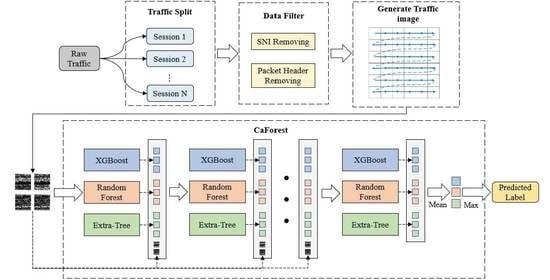
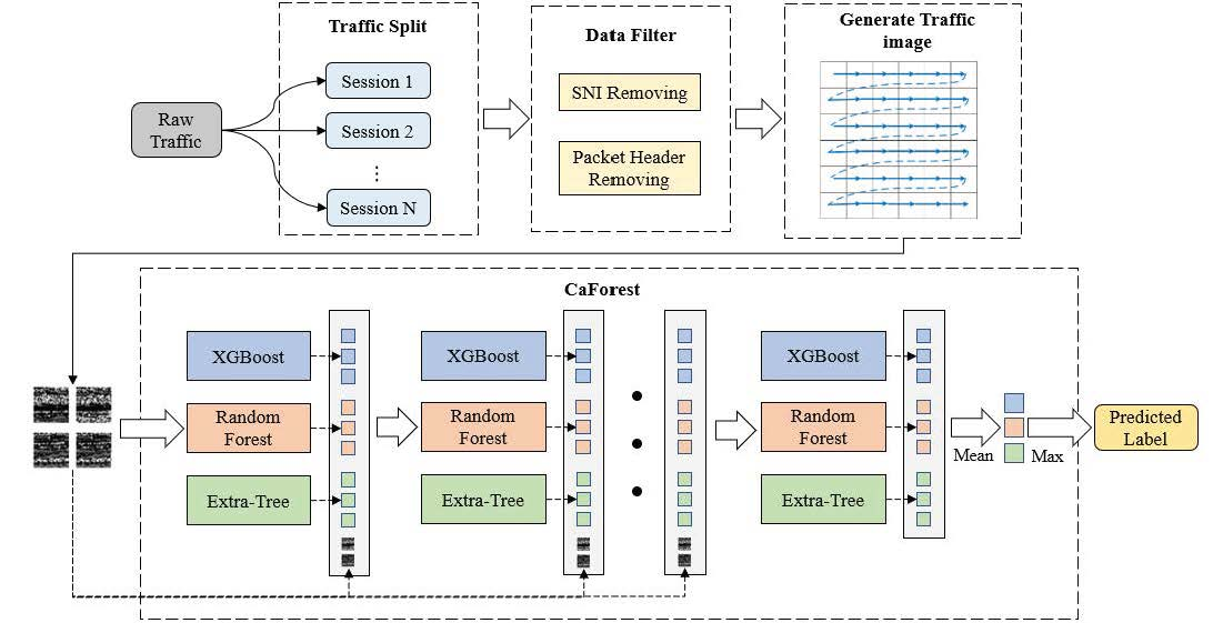
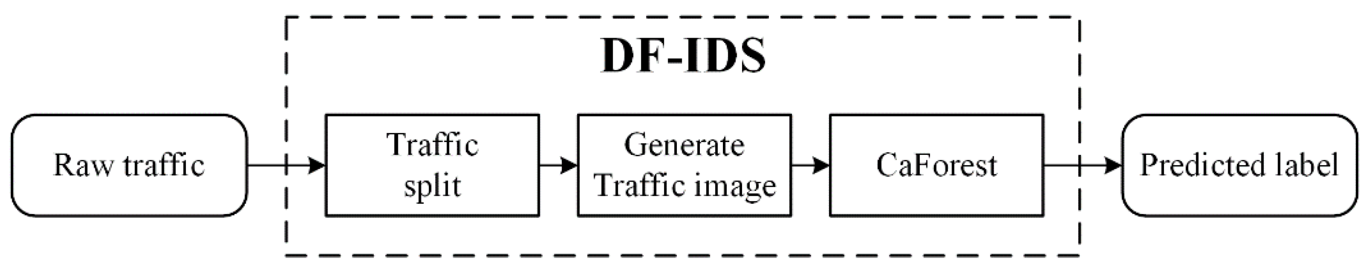
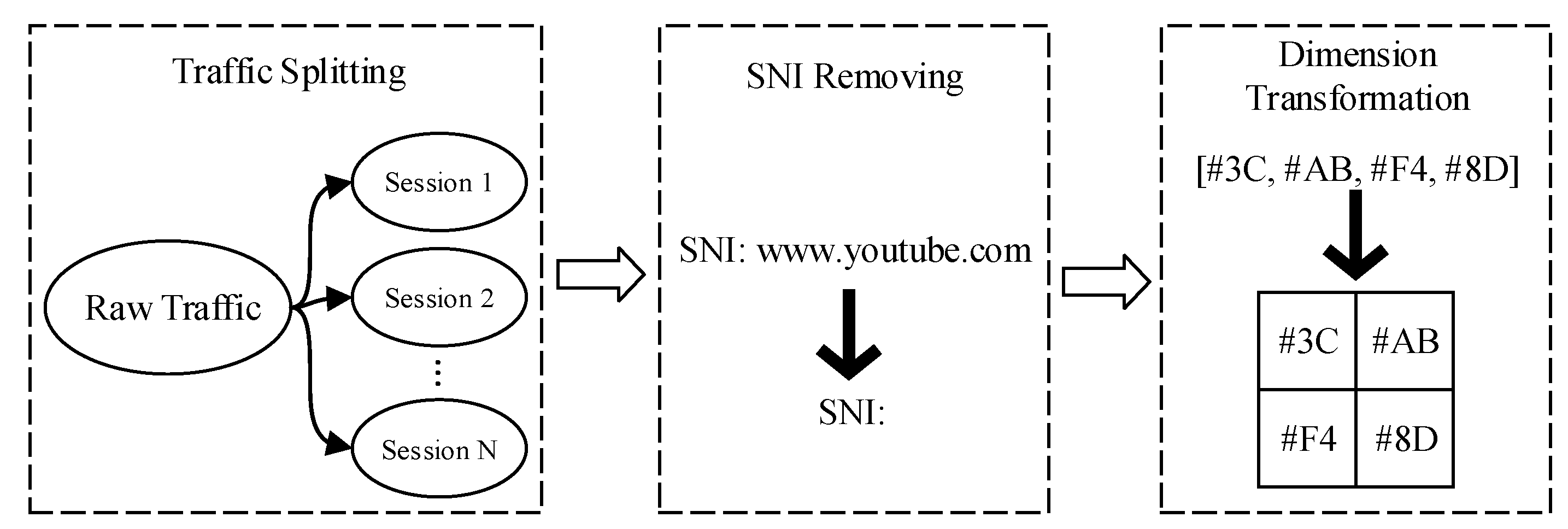
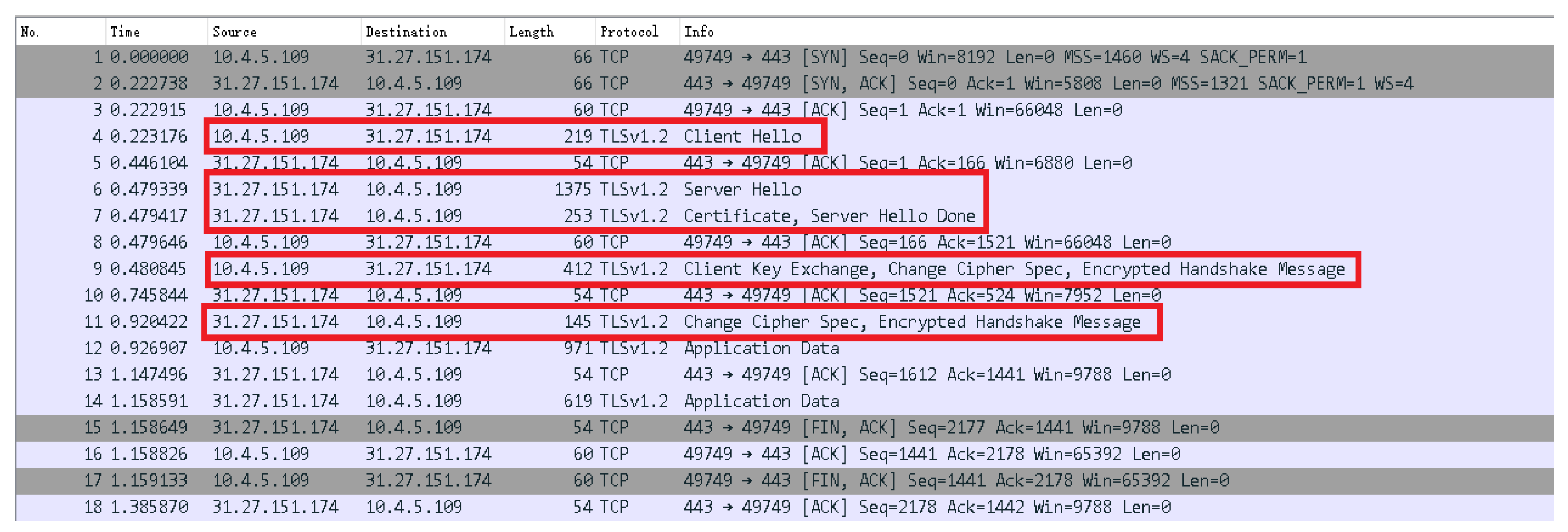
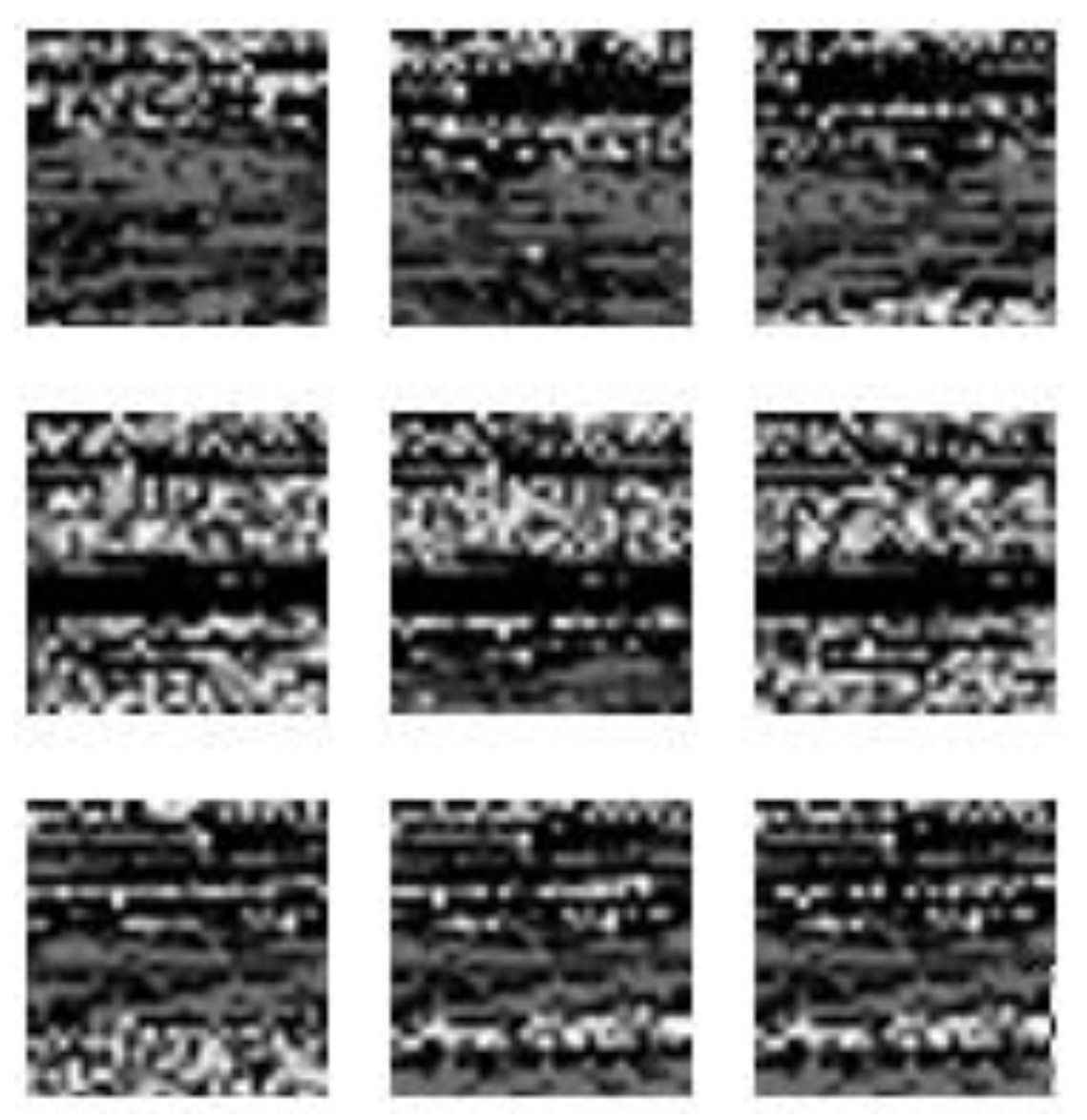
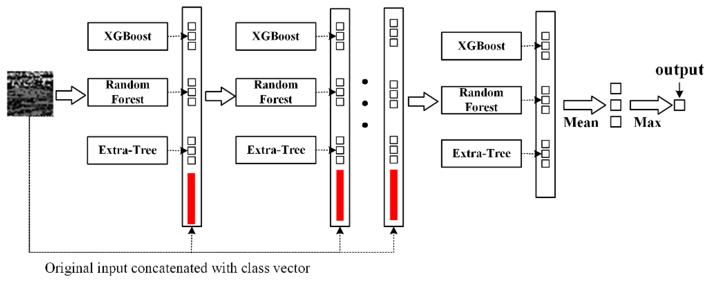
The scope of this paper is detection of network intrusion. The purpose of the proposed work was to solve the existing deep-learning models’ problem due to a lack of data. The main contribution of this paper was to propose a deep-forest-based anomaly-intrusion detection framework named DF-IDS for small-scale and unbalanced SSL/TLS encrypted malicious traffic. In this framework, firstly, according to the characteristics of SSL/TLS-encrypted malicious traffic, the original traffic was split into sessions and converted to a traffic image as the input of the detector. Then, based on deep-forest technology, and considering both the detection accuracy and efficiency, an improved gcForest framework named CaForest was designed. This framework could integrate various type of base classifiers, and the depth of model could automatically adjust according to the data. DF-IDS realized high-precision encrypted malicious traffic detection on small-scale and unbalanced data.

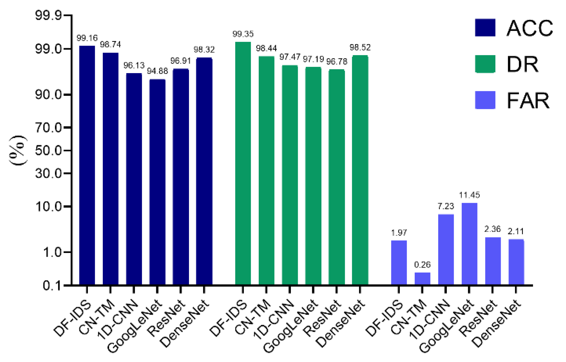
The remainder of this paper is organized as follows. Section 2 introduces work related to encrypted traffic detection. Section 3 presents our DF-IDS method, including the data-preprocessing method and the design of the detection model. Section 4 presents the experiments and results to evaluate our method, and we compare our method with other works. Section 5 closes with our conclusions and plans for future work.

Table 1. Summary of acronyms in this paper.

Acronym	Definition
SSL	Secure Socket Layer
TLS	Transport Layer Security
CNN	Convolutional neural network
SAE	Stacked autoencoder
LSTM	Long short-term memory
1D	One-dimensional
DNS	Domain name system
HTTP	HyperText Transfer Protocol
CART	Classification and regression tree
K-NN	K-nearest neighbors
IDS	Intrusion detection system
SNI	Server name indication
SVM	Support vector machine
RF	Random forest

shows all acronyms used in this paper.

2. Related Work

With the development of deep-learning technology, many researchers have applied it to encrypted traffic classification. Most studies currently available were focused on the classification of benign network traffic, such as video flow, chat flow, file flow, and so on. Lotfollahi et al. [9] used a stacked autoencoder (SAE) and a 1D convolutional neural network (1D-CNN) to detect encrypted benign traffic. They extracted the first 1500 bytes starting from the IP header of each packet, masked the IP address and port number, then applied SAE or 1D-CNN to train the classifiers. In this work, a single packet was used as the input sample, so the sequential correlation of the entire flow was not well utilized. Vu et al. [10] extracted the head of a packet starting from the IP layer and the first n bytes of payload, and utilized long short-term memory (LSTM) as the classification model; this method achieved a high F1 score of 0.98. However, since different types of encrypted traffic have specific IP addresses and port numbers in the head of network packets, the classification results may have been affected by these factors [9]. Wang et al. [11] proposed an end-to-end encrypted traffic-classification method based on 1D-CNN. They extracted the first 784 bytes of each flow or session as the input, and achieved a precision of 85.8% and a recall of 85.9% in a 12-classification experiment. Zou et al. [12] proposed a cascade model of CNN and LSTM. They used any three consecutive packets in a session and extracted the first 784 bytes of each packet starting from the IP layer, then reshaped these data into a 2D image as the input. Here, CNN was used to extract spatial features, and LSTM was adopted to find the temporal relevancies of the spatial features. Using the same dataset as a reference [11], the average precision and recall were increased by 5%. Lopez-Martin et al. proposed a classification model named gaNet-C [13] by using hyperbolic tangent (tanh) layers as the final layer of each “building block”, adding a sigmoid fully connected (FC) layer prior to any network output, and applying a log loss instead of a quadratic loss as the cost function. Experiments on an unbalanced dataset showed that the accuracy of gaNet-C could achieve 94%, the recall was 60%, and the precision was 85% in binary classification. Zeng et al. [14] proposed a framework called deep-full-range (DFR), in which 1D-CNN, LSTM, and SAE were employed. They extracted the first 900 bytes of each data file as the input. The experiments on the ISCX VPN-non VPN traffic dataset showed that the model’s performances based on 1D-CNN and LSTM were better than that of SAE.

At present, the features used for encrypted malicious traffic detection are mainly based on statistical characteristics. Prasse et al. [15] combined byte-related features, time-related features, and domain name features to train an LSTM-based classifier. Their experiments showed that the performance of the detector with combined features was better than that of the detectors using a single type of feature. In their method, the domain name was used; however, since the domain name is easier to be modified or forged by attackers, a detector trained with this information may be easily fooled. Anderson et al. [16] considered that different software had different preference when using protocols such as TLS, domain name system (DNS) and Hypertext Transfer Protocol (HTTP), so they used not only statistical features, but also TLS handshake metadata, DNS contextual flow linked to the encrypted flow, and the HTTP headers of the HTTP contextual flow. The experiments showed that their work effectively reduced the false-alarm rate. This work proved that the SSL/TLS handshake metadata was useful in detecting SSL/TLS-encrypted malicious traffic. In addition, Anderson et al. [17] extracted 22 standard features for TLS-encrypted session traffic based on Williams’ work [18], and enhanced them to obtained 319 enhanced features. Six common machine-learning algorithms, such as support vector machine (SVM), random forest (RF), and decision tree, were used to build models. The experiments on two large-scale datasets showed that, with the enhanced features, the performance of the classifiers were improved, and models based on a decision tree or RF had better classification accuracies. Shekhawat et al. [19] proposed to use byte-related features, time-related features and SSL/TLS-protocol-related features. They conducted classification with SVM, RF, and XGBoost, and achieved accuracies of 91.22%, 99.8%, and 99.88%, respectively, in binary classification. Their experiments showed that the decision tree ensemble model performed better than SVM. This work also proved that SSL/TLS protocol information is useful for classification. Stergiopoulos et al. [20] selected the size of packet, the size of payload, the size ratio of payload to packet, the size ratio of current packet to previous packet, and the interarrival time as features. They used a classification and regression tree (CART) decision tree and the K-NN (k-nearest neighbors) algorithm as classifiers, and achieved an accuracy of 94.5% in a binary-classification experiment. However, in the case of small-scale data, the accuracy dropped to 88.8%.

A summary of related works and ours are shown in

Table 2. Summary of related work.

Paper	Concerns	Methodology	Inference Task	Deep-Learning or Machine-Learning Family	Input Unit	Feature	Dataset Size
Lotfollahi et al. [7]	TC	End-to-End	MCC	SAE and 1D-CNN	Packet	-	M
Vu et al. [8]	TC	End-to-End	MCC	LSTM	Packet	-	S
Wang et al. [9]	TC	End-to-End	MCC	1D-CNN	Flow/Session	-	L
Zou et al. [10]	TC	End-to-End	MCC	CNN + LSTM	Session	-	L
Zeng et al. [13]	TC and MTD	End-to-End	MCC	CNN + LSTM + SAE	Flow	-	M
Prasse et al. [14]	MTD	Feature-based	BC	LSTM	-	BR, TR, and O	L
Anderson et al. [15]	MTD	Feature-based	BC	L1-LR	-	BR, TR, and PR	L
Anderson et al. [16]	MTD	Feature-based	BC	SVM, RF, DT, and O	-	BR, TR, and PR	L
Shekhawat et al. [18]	MTD	Feature-based	BC	SVM, RF, and XGB	-	BR, TR, and PR	L
Stergiopoulos et al. [19]	MTD	Feature-based	BC	CART and K-NN	-	BR and TR	L
Ours	TC and MTD	End-to-End	MCC	DF	Session	-	S

Abbreviations: TC, traffic classification; MTD, malicious traffic detection; BC, binary classification; MCC, multiclass classification; CNN, convolutional neural network; 1D-CNN, one-dimensional CNN; SAE, stacked autoencoder; LSTM, long short-term memory; CART, classification and regression tree; K-NN, k-nearest neighbors; SVM, support vector machine; RF, random forest; XGB, XGBoost; L1-LR, L1-logistic regression; DT, decision tree; O, others; BR, byte-related; TR, time-related; PR, protocol-related. For the dataset size (the number of samples in the minimum category): S, less than 1000; M, 1000–10,000; L, more than 10,000.

. It can be seen that most studies were focused on the classification of benign application traffic in end-to-end mode, or benign and malicious binary classification in feature-based methodology. Only a few studies aimed at malicious multiclassification in end-to-end mode. At the same time, although many studies realized classification of encrypted traffic based on a deep-learning method, which proved the effectiveness of the deep-learning method in the task of encrypted traffic classification, these works were all based on a large number of samples. Since the main characteristic of a deep-learning-based classifier is its reliance on a large number of training samples, when the number of training samples is insufficient, such as 1000 samples or less, a model based on deep learning can easily fall into overfitting, making it difficult to obtain a high detection accuracy. In view of this problem, we designed a novel deep-forest-based algorithm for encrypted malicious traffic with small-scale and imbalanced data.

3. Proposed Method

Aiming at the problem of detecting SSL/TLS encrypted malicious traffic with small-scale and unbalanced training data, a deep-forest-based detection method named DF-IDS was designed in this study. The workflow of DF-IDS is shown in Figure 1.

At first, the raw traffic was split according to the characteristics of the SSL/TSL protocol, then the traffic image was generated as the input of the detector. Based on the deep-forest framework, an improved classifier named CaForest was constructed to detect encrypted malicious traffic.

3.1. Preprocess of Network Traffic

Figure 2 shows the flow of processing of traffic.

3.1.1. SSL/TLS-Encrypted Traffic Splitting

SSL/TLS is a protocol that is widely used for encrypted transmission. SSL/TLS uses a mixture of symmetric encryption and asymmetric encryption technology. When using the SSL/TLS protocol, the client side and server side must first finish the handshake process, and then transmit encrypted application data to each other. In the handshake stage, the traffic contains unencrypted data such as the protocol version, authentication information, and key exchange information. Some studies showed that this information could help to identify encrypted malicious traffic effectively [16,19,21].

Usually, the captured raw traffic can be split into basic units in terms of packet, flow, or session for detection. Considering that the session contains all of the useful information [11,12], the session was adopted as the basic traffic unit in this study. The raw traffic was split according to session using 5-tuple information: source IP, source port, destination IP, destination port, and transport layer protocol.

An example of part of a session is shown in Figure 3; the red boxes denote handshake information.

3.1.2. Traffic Processing

After the traffic was split according to the 5-tuple information, in order to avoid some special information interfering with the classification, further processing was needed. Firstly, the packet header was removed, and only the traffic payload was kept in order to avoid the effects caused by the IP address, port number, etc. This information may cause overfitting of the model. Then, considering that some Hypertext Transfer Protocol Secure (HTTPS) sessions contain an unencrypted server name indication (SNI) field in the handshake data, which states the domain name to be visited, and might interfere with the classification result, this field was removed as well. Finally, since some researchers have shown that they are sufficient for a deep-learning-based classifier [9,11,12], the first n bytes in a session also were extracted.

3.1.3. Traffic Image

Deep-learning classifiers usually use a two-dimensional image as input, and automatically extract the nonlinear features hidden in the image through a deep neural network to achieve end-to-end classification. A deep-forest model can use both two-dimensional and one-dimensional input data. Considering the need for comparison experiments, here, the traffic was converted to a two-dimensional image called the traffic image.

The raw traffic captured by tools such as Wireshark is essentially a sequence of bytes. A byte is a binary hexadecimal number, and its corresponding decimal value range is 0–255, which are just the intervals of a pixel’s gray value. Therefore, each byte in traffic can be converted into a pixel in a grayscale image. According to the route (from top to bottom and from left to right) in Figure 4, the traffic is converted to a two-dimensional image as shown in Figure 5, and is then used as the input for the deep-learning classifier. In this process, there is no loss of information in the original data.

3.2. Detection Model

3.2.1. CaForest-Based Classifier

Deep forest (DF) was proposed by Zhou in 2017 [22]. It is unlike the traditional deep-learning method, which stacks neural networks, while DF stacks forest models. In contrast to most DNNs whose model complexity is fixed, gcForest adaptively decides its own model complexity by terminating training when adequate. This enables its applicability at different scales of training data, so it is not limited to large scales. The implementation framework of DF proposed by Zhou is called gcForest, which has proved suitable in the classification of small-scale and unbalanced data [23]. Compared with a model based on a DNN, gcForest has fewer hyperparameters and better robustness [24].

There are two main parts in the gcForest framework: multi-grained scanning and cascade forest [22]. The first part is similar to the convolutional layer in CNN. It uses a sliding window to scan the input image and extract the texture feature. The cascade forest utilizes a stacking algorithm. As is shown in Figure 5, the traffic image has no typical image texture, since the entropy of the encrypted data is very high [25]. In addition, unlike the usual image, the traffic image does not contain much redundant information, and each pixel in the image represents a certain byte in the traffic [16]. Extracting texture features might cause information loss. Meanwhile, considering that multigrained scanning will greatly increase the time and memory costs in the training period, only the part of cascade forest in the gcForest framework was kept when building the detection model in this study. This simplified framework was named CaForest. The structure of CaForest is shown in Figure 6.

The gcForest framework can integrate various type of base classifiers, and allows user to freely design the types and numbers of base classifiers. The depth of cascade forest can automatically adjust during the training process. In CaForest, each layer of cascade forest realizes an ensemble of base classifiers. Some researchers have proved that the combination of tree ensemble models, such as gcForest, random forest, Extra Trees and XGBoost, is effective [16,24]. This can overcome overfitting by bootstrapping, pruning and feature-sampling strategies.

The output of each base classifier is called the class vector, which is a probability vector. The dimensions of the class vector are equal to the number of classes, and the value of each dimension is the probability that the sample belongs to the corresponding class. In the process of forward propagation, the class vectors generated by the base classifiers are concatenated with the original input and are the input of the next layer. In the last layer, a mean class vector of all the class vectors generated by base classifiers is calculated, and then the model chooses the class with the highest probability as the predicted label of the input sample.

3.2.2. Random Forest (RF)

Random forest is a bagging model that contains many decision-tree models. In random forest, each tree is trained and makes prediction independently. The final decision is determined by a voting mechanism. In random forest, two random subsets—a random subset of the original training set and random subset of the original feature set—are introduced to guarantee the diversity of the base classifier and avoid overfitting.

Assuming that a random forest contains N decision trees, the original training set is $D$, and the feature set is $V$. Through a bootstrapping algorithm, random forest constructs N subsets of $D$:$\left\{{\mathrm{D}}_1, {\mathrm{D}}_2,{\mathrm{D}}_3\dots {\mathrm{D}}_N\right\}$. N decision trees are generated independently with the N subsets. Node splitting is an important part in the growing of a decision tree. In random forest, instead of searching the whole feature set $V$ for node splitting, each decision tree randomly selects a subset V_sub of $V$ to search for the best splitting feature. When each tree is trained, random forest obtains a final prediction by voting. Let $T_k$ denote the prediction result of tree k, and the final prediction of sample $x_i$ is obtained through Equation (1):

$${\widehat{y}}_i=\underset{y}{\arg \max }{\displaystyle \sum _{k=1}^N\mathrm{I}(T_k(x_i)=y)}$$

(1)

where:

$$\mathrm{I}(T_k(x_i)=y)=\{\begin{array}{l}1, if T_k(x_i)=y\\ 0, if T_k(x_i)\ne y\end{array}$$

(2)

Random forest usually uses a classification and regression tree (CART) decision tree as the base classifier. The CART algorithm adopts the Gini index to evaluate the information gain of a splitting feature and its value. Assuming that there are K classes, and the probability of the k-th class is $p_k$, the Gini index then is calculated as follows:

$$\mathrm{Gini}(p)={\displaystyle \sum _{k=1}^K{p}_k(1-p_k)}=1-{\displaystyle \sum _{k=1}^K{p}_k{}^2}$$

(3)

If the sample set $D$ is split into $D_1$ and $D_2$, the value of feature A is equal to a, and the Gini index of set $D$ is defined as:

$$\mathrm{Gini}(D,A=a)=\frac{\left|D_1\right|}{\left|D\right|}\mathrm{Gini}(D_1)+\frac{\left|D_2\right|}{\left|D\right|}\mathrm{Gini}(D_2)$$

(4)

3.2.3. Extra Trees

Extra Trees is also a bagging model. Unlike random forest, it uses a complete training set $D$ to train each tree. In the process of node splitting, it uses a random subset of the feature set, and selects the splitting-feature value randomly.

Extra Trees also adopts a CART decision tree as the base classifier. In random forest, for any feature $A$, the model traverses every possible value $a_i$ of $A$, and calculates $\mathrm{Gini}\left(D,A=a_i\right)$, then chooses $a_i^{*}$, which minimizes the $\mathrm{Gini}\left(D,A=a_i\right)$ as the best splitting value of feature $A$. However, in Extra Trees, the best splitting value $a_i^{*}$ of feature $A$ is not obtained only by calculating, but also by randomly selecting.

3.2.4. XGBoost

XGBoost takes advantage of a boosting algorithm to reduce bias to improve the performance of the model. The XGBoost model also consists of a CART decision tree, and can be described by Equation (5):

$${\widehat{y}}_i={\displaystyle \sum _{k=1}^K{f}_k(x_i)}$$

(5)

where $f_k$ represents the k-th tree. Trees in XGBoost are generated iteratively. Each tree fits the residual of previous model; that is:

$$f_K=y_i^{}-{\displaystyle \sum _{k=1}^{K-1}{f}_k(x_i)}$$

(6)

where $y_i$ is the actual value of sample $x_i$. When XGBoost generates a new tree $f_t$ in the t-th round, the objective function of XGBoost is given as Equation (7):

$$obj(\theta )={\displaystyle \sum _i^{n}l(y_i,{\widehat{y}}_i{}^{(t-1)}+f_t(x_i))+\gamma T+\frac{1}{2}\lambda {\displaystyle \sum _{j=1}^T{w}_j^2}}+C$$

(7)

where T is the number of leaf nodes, $w_j$ is the output value of the j-th leaf node, and $\gamma$ and $\lambda$ are weights. The first term of the objective function is the loss function of the model, and the second and third terms are the regularization terms, which are used to restrict the complexity of the tree and prevent overfitting. XGBoost generates a new tree by minimizing the objective function. A second-order Taylor’s expansion is performed on Equation (7) when $f_t(x_i)=0$. After simplification, the calculation of output value $w_j$ of leaf node and the final objective function $Obj*$ are obtained:

$$\begin{array}{l}{w}_j^{*}=-\frac{G_j}{H_j+\lambda }\\ Ob{j}^{*}=-\frac{1}{2}{\displaystyle \sum _{j=1}^T{w}_j^{*}}+\gamma T\end{array}$$

(8)

XGBoost grows new trees iteratively based on Equation (8).

3.3. Training Process of CaForest

The initial number of layers in CaForest was 0. At the beginning of the training process, the first layer was trained with the original training data. Then, the output of the first layer was concatenated with the original input, which was used to train the second layer. When the training of one layer was completed, the algorithm automatically determined whether to add the next layer according to the improvement in the classification accuracy. If the accuracy of the model had no obvious improvement, the training ended. The model training process was shown in Algorithm 1.

Algorithm 1: Training process of CaForest model

Input: training set $D^0=\left\{x_1,x_2,x_3\dots \dots x_{\left|D\right|}\right\}$;

Output: model $\mathrm{M}={{\displaystyle \sum }}_{i=1}^{\left|M\right|}{M}_i$; where ${\displaystyle \sum }$ represents cascading;

Parameters: $\left|D\right|$ is the number of sample; N is the number of classes; K is number of base classifiers in each layer; $\left|M\right|$ is the depth of model; $M_i$ is the i-th layer of the model; $\oplus$ represents cascading;

do:

$\mathrm{M}\ne \varnothing$; $\left|M\right|$ = 0; i = 0;//Initialization

while(1)

if $\mathrm{M}\ne \varnothing$: //Output Model

calculate the accuracy of M through cross-alidation.

if the accuracy of the model has no obvious improvement in the q–th round (q = 3)

output M;

break;

else: //Training

$\left|M\right|$ + 1; i + 1; training $M_i$ with $D^{i-1}$; $M=M\oplus M_i$;

for $x_d$ in $D^{i-1}$:

$M_i$ outputs K N-dimention class vectors of $x_d$, concatenates them with $x_d$, obtains vector $x_d^i$;

obtains new training set $D^i=\left\{x_1^i,x_2^i,x_3^i\dots \dots x_{\left|D\right|}^i\right\}$;

4. Experiments and Results

4.1. Dataset, Evaluation Metrics, and Experimental Environment

4.1.1. Dataset Description

Three real-life datasets were used in this paper:

Dataset 1: In this dataset, the encrypted traffic was collected from the MCFP dataset [26]. Referring to the research of other scholars [20,27], and considering the proportion of SSL/TLS sessions to all the sessions and the integrity of the captured sessions, eight types of malicious traffic (Nos. 1, 8, 25, 46, 50, 83, 110, and 140) were selected from the MCFP dataset. Since the dataset did not provide the name of the attack, they were named M1 to M8 here. The normal traffic was undersampled from the ISCX VPN-nonVPN [28] dataset, which contained 14 types of nonmalicious encrypted traffic. The number of sessions of each class is shown in

Table 3. Sample numbers of Dataset 1.

	M1	M2	M3	M4	M5	M6	M7	M8	Normal
#N	500	2000	1900	72	800	800	900	1000	3368
#P	4.41%	17.6%	16.8%	0.62%	7.05%	7.05%	7.94%	8.81%	29.7%

.

Dataset 2: In this dataset, the encrypted ransomware traffic was collected from the following three websites: http://www.malware-traffic-analysis.net (accessed on 15 March 2021), https://packettotal.com (accessed on 15 March 2021), and https://app.any.run (accessed on 15 March 2021). Three types of ransomware were selected: cerber, cryptowall, and gandcrab. The normal traffic came from the Monday subset of the CICIDS2017 dataset [29]. The number of sessions of each class is shown in

Table 4. Sample numbers of Dataset 2.

	Cerber	Cryptowall	Gandcrab	Normal
#N	569	1161	4172	20,000
#P	2.2%	4.48%	16.1%	77.21%

.

Dataset 3: In this dataset, three types of malicious traffic, named 2020 Emotet, 2020 TA551, and 2019 Ursnif, were collected from https://malware-traffic-analysis.net/index.html (accessed on 15 March 2021). Compared with Datasets 1 and 2, the types of attack were newer. The normal traffic was from the 2017 CTU-Normal-32 dataset [30]. The number of sessions of each class (#N) is shown in in

Table 5. Sample numbers of Dataset 3.

	Emotet	TA551	Ursnif	Normal
#N	191	325	790	4499
#P	3.29%	5.59%	13.6%	77.5%

. Here, #P represents the proportion of the number of sessions of each class in the total number of sessions.

It can be seen that the amounts of some samples in these datasets were small, such as M4, Cerber, and Emotet. The distribution of samples in these datasets was unbalanced.

4.1.2. Evaluation Metrics

The accuracy (ACC), detection rate (DR), and false-alarm rate (FAR) were used as the evaluation metrics:

$$\begin{array}{c}\mathrm{ACC}=\frac{TP+TN}{TP+FP+TF+FN}\times 100\%\\ \mathrm{DR}=\frac{TP}{TP+FN}\times 100\%\\ \mathrm{FAR}=\frac{FP}{FP+TN}\times 100\%\end{array}$$

(9)

where TP is the number of instances correctly classified as positive, TN is the number of instances correctly classified as negative, FP is the number of instances incorrectly classified as positive, and FN is the number of instances incorrectly classified as negative.

4.1.3. Experimental Environment

The experiments were conducted on a Dell T630 server with an Ubuntu 18.04 64-bit OS and 32 GB of RAM. An NVIDIA GTX 1080Ti GPU with 11 GB of VRAM was used for acceleration.

4.2. Experimental Results

4.2.1. Experiment on Input Size

The purpose of this experiment was to verify the impact of the first n bytes extracted from a session (i.e., the size of traffic image) on the detection result. This experiment was executed on Dataset 1; the dataset was divided into a training set, validation set, and test set at proportions of 60%, 15%, and 25%, respectively, and each tree ensemble model (XGBoost, random forest, and Extra Trees) in CaForest consisted of 10 decision trees.

Table 6. Results of binary classification with different input sizes.

Input Size	ACC	DR	FAR
16 × 16	97.46%	98.00%	3.94%
28 × 28	98.41%	98.95%	3.02%
32 × 32	97.97%	99.15%	5.13%
48 × 48	97.72%	98.45%	4.21%
64 × 64	96.96%	97.95%	5.65%
96 × 96	96.56%	97.65%	6.32%
128 × 128	96.45%	97.35%	5.92%

and

Table 7. Results of nine-class classification with different input sizes.

Input Size	ACC	M-DR	M-FAR
16 × 16	92.07%	83.71%	1.11%
28 × 28	93.30%	92.14%	0.91%
32 × 32	93.81%	92.53%	0.85%
48 × 48	93.66%	92.28%	0.87%
64 × 64	93.19%	92.17%	0.93%
96 × 96	92.83%	92.30%	0.98%
128 × 128	92.14%	90.43%	1.09%

show the experimental results of the binary classification and nine-class classification, respectively. In the tables, M-DR and M-FAR are the mean values of DR and FAR, respectively.

As can be seen in Table 6 and Table 7, in the binary-classification experiment, when the input size was 28 × 28, the ACC was the highest, at 98.41%, and the FAR was the lowest, at 3.02%. When the input size was 32 × 32, the DR was the highest, at 99.15%. In the nine-class classification experiment, when the input size was 32 × 32, the ACC, M-DR, and M-FAR were all the best (93.81%, 92.53%, and 0.85%, respectively). When the image size was larger than 32 × 32, the ACC and DR/M-DR in both the binary and nine-class classification experiments decreased, while the M-FAR in the nine-classification experiment increased. Therefore, 32 × 32 (i.e.,1024 bytes) was selected as the size of the input image for the detection model in subsequent experiments.

Moreover, from this experiment, it could be seen that the detection performance of the model decreased with an increase in the input size. This showed that the handshake information in SSL/TLS plays a more important role in encrypted traffic detection.

4.2.2. Experiment on CaForest Structure

The type of base classifiers in each layer of CaForest are the main factors that influence the performance of the detector. The purpose of this experiment was to choose the base classifiers, and to seek the optimal number of decision trees. This experiment was executed on Dataset 1.The results of the binary classification and nine-class classification experiments are shown in

Table 8. Results of binary classification with different CaForest structures.

	q = 5			q = 10			q = 15			q = 20
	ACC	DR	FAR	ACC	DR	FAR	ACC	DR	FAR	ACC	DR	FAR
X	97.4%	97.7%	3.55%	97.7%	98.6%	4.47%	98.0%	98.7%	3.55%	98.2%	99.1%	4.08%
R	98.8%	99.3%	2.5%	98.9%	99.3%	2.11%	98.8%	99.3%	2.37%	99.0%	99.3%	1.84%
E	98.5%	99.1%	2.89%	98.8%	99.5%	3.16%	98.3%	99.3%	4.34%	98.6%	99.5%	3.68%
X + R	97.9%	98.8%	4.47%	98.0%	98.9%	4.47%	98.4%	99.3%	3.95%	98.4%	99.4%	4.08%
X + E	97.8%	98.3%	3.68%	98.3%	98.7%	2.89%	97.9%	98.9%	4.87%	98.0%	98.8%	4.34%
R + E	98.6%	99.2%	3.03%	98.8%	99.4%	2.5%	99.0%	99.4%	1.97%	99.1%	99.5%	1.97%
X + R + E	97.6%	98.6%	5.00%	98.0%	99.2%	5.13%	98.2%	98.7%	3.16%	98.5%	99.3%	3.55%

and

Table 9. Results of nine-class classification with different CaForest structures.

	q = 5			q = 10			q = 15			q = 20
	ACC	M-DR	M-FAR	ACC	M-DR	M-FAR	ACC	M-DR	M-FAR	ACC	M-DR	M-FAR
X	93.4%	92.5%	0.92%	93.6%	91.9%	0.90%	94.3%	92.9%	0.80%	94.2%	92.8%	0.82%
R	93.1%	89.5%	0.97%	93.8%	90.9%	0.85%	94.3%	93.4%	0.77%	94.5%	93.6%	0.75%
E	88.0%	79.6%	1.80%	89.9%	82.7%	1.47%	89.6%	83.7%	1.52%	90.0%	84.9%	1.45%
X + R	93.3%	92.5%	0.94%	93.4%	92.1%	0.90%	94.5%	93.4%	0.76%	94.4%	93.3%	0.77%
X + E	93.4%	92.8%	0.90%	93.7%	92.4%	0.87%	94.5%	93.2%	0.75%	94.5%	93.3%	0.76%
R + E	93.1%	90.7%	0.97%	94.3%	94.2%	0.77%	94.2%	93.8%	0.80%	94.9%	94.4%	0.70%
X + R + E	93.6%	92.4%	0.88%	93.8%	92.5%	0.85%	94.3%	93.3%	0.77%	94.3%	93.3%	0.78%

, respectively. In the tables, X, R, and E represent the XGBoost, random forest, and Extra Trees classifiers, respectively; q represents the number of decision trees in each base classifier; and M-DR and M-FAR represent the mean values of DR and FAR, respectively, in the multiclass classification experiments.

It can be seen in Table 8 that the ACC and DR of R + E were the highest when q = 20, at 99.1% and 99.5%, respectively. When q = 10 and q = 20, the DR of E was the highest, at 99.5%. When q = 20, the FAR = 1.84% of R was the lowest. In addition, it can be seen in Table 9 that in the nine-class classification experiment, the combination of random forest and Extreme Trees, which consisted of 20 decision trees, achieved the best detection result, and the three indices of ACC, M-DR, and M-FAR were all the best, at 94.9%, 94.4%, and 0.70%, respectively. Therefore, random forest and Extreme Random Trees, which consisted of 20 decision trees, were selected as the base classifiers in each layer of the CaForest model in the following experiments. So, in the hyperparameters of our model, the number for random forest was 1, the number for Extreme Random Tree was 1, and the number of forests was 20.

4.2.3. Comparison Experiments of Binary Classification

To validate the effectiveness of the proposed model in the binary-classification case, a 1D-CNN proposed in [9], a CNN + LSTM (later called CN-TM) proposed in [10], GoogLeNet, ResNet [31], and DenseNet [32] models were compared with our DF-IDS detector. The experiment results of the binary classification of Dataset 1 are shown in Figure 7 and Figure 8.

As can be seen in Figure 7, the ACC and DR of DF-IDS were the highest, and its FAR was only higher than CN-TM. In addition, it can be seen in the ROC curve in Figure 8 that DF-IDS had the best performance.

The amounts of RAM occupied by these models were also compared, and the results are shown in Figure 9.

It can be seen that the amount of RAM occupied by the DF-IDS model was larger than that of DenseNet and GoogLeNet, but was smaller than other models.

In this experiment, the training time of DF-IDS was 19.39 s, and the testing time was 3.67 s.

4.2.4. Comparison Experiments of Multiclass Classification

To further validate the effectiveness of the proposed model in the multiclassification case, 1D-CNN, CNN + LSTM, GoogLeNet, ResNet, and DenseNet models were compared with DF-IDS using three datasets. The experiment results of multiclassification using Datasets 1, 2, and 3 are shown in

Table 10. Performance of multiclassification model using Dataset 1.

(a) DR Results
Model	M1	M2	M3	M4	M5	M6	M7	M8	Normal	M-DR
DF-IDS	92.9%	84.1%	93.5%	100%	97.5%	94.4%	97.6%	90.6%	98.9%	94.4%
CN-TM	38.9%	100%	96.2%	5.26%	95.5%	95.0%	91.6%	90.4%	100%	79.2%
1D-CNN	11.9%	79.2%	80.9%	15.8%	96.0%	74.6%	71.7%	77.7%	94.5%	66.9%
GoogLeNet	8.7%	55.7%	52.5%	10.5%	95.0%	72.1%	75.7%	74.5%	88.0%	59.2%
ResNet	33.3%	84.5%	71.1%	89.4%	96.5%	76.0%	96.4%	77.6%	96.1%	80.1%
DenseNet	56.1%	87.3%	79.5%	92.6%	97.3%	77.7%	74.4%	82.7%	94.2%	82.4%
(b) FAR Results
Model	M1	M2	M3	M4	M5	M6	M7	M8	Normal	M-FAR
DF-IDS	0.67%	0.65%	0.65%	0.00%	0.00%	0.96%	1.75%	0.96%	1.11%	0.70%
CN-TM	0.59%	0.29%	3.49%	0.12%	0.75%	0.79%	0.79%	0.71%	0.05%	0.84%
1D-CNN	0.27%	8.99%	6.14%	0.00%	0.73%	1.52%	1.81%	2.88%	5.78%	3.13%
GoogLeNet	1.92%	14.42%	13.75%	0.00%	1.44%	1.51%	5.30%	4.50%	3.96%	5.20%
ResNet	0.77%	1.85%	1.27%	0.00%	0.13%	0.69%	9.16%	0.81%	5.46%	2.24%
DenseNet	2.60%	6.41%	1.14%	0.03%	0.22%	1.10%	1.91%	3.24%	3.17%	2.21%

,

Table 11. Performance of multiclassification model using Dataset 2.

(a) DR Results
Model	Cerber	Cryptowall	Gandcrab	Normal	M-DR
DF-IDS	92.1%	92.9%	98.6%	99.9%	95.9%
CN-TM	77.1%	84.9%	98.8%	99.9%	90.1%
1D-CNN	56.1%	83.9%	96.4%	99.9%	84.1%
GoogLeNet	73.6%	92.4%	97.6%	99.7%	90.8%
ResNet	81.5%	88.2%	97.3%	99.7%	91.6%
DenseNet	85.1%	93.3%	97.9%	100%	94.0%
(b) FAR Results
Model	Cerber	Cryptowall	Gandcrab	Normal	M-FAR
DF-IDS	0.13%	0.04%	0.48%	0.53%	0.29%
CN-TM	0.07%	0.26%	1.15%	0.18%	0.42%
1D-CNN	0.08%	0.57%	1.07%	3.59%	1.33%
GoogLeNet	0.07%	0.61%	0.88%	0.36%	0.48%
ResNet	0.33%	0.40%	0.74%	0.81%	0.57%
DenseNet	0.07%	0.32%	0.39%	0.97%	0.44%

and

Table 12. Performance of multiclassification model using Dataset 3.

(a) DR Results
Model	Emotet	TA551	Ursnif	Normal	M-DR
DF-IDS	91.6%	95.1%	100%	100%	96.7%
CN-TM	0%	0%	27.6%	95.2%	30.7%
1D-CNN	97.6%	38.7%	99.5%	100%	83.95%
GoogLeNet	77.08%	93.9%	99.49%	100%	92.62%
ResNet	0%	0%	0%	100%	25%
DenseNet	97.9%	95.1%	100%	100%	98.25%
(b) FAR Results
Model	Emotet	TA551	Ursnif	Normal	M-FAR
DF-IDS	0.28%	0.21%	0.08%	0%	0.14%
CN-TM	0%	0%	5.7%	82.5%	22.05%
1D-CNN	3.48%	0.07%	0%	0.75%	1.07%
GoogLeNet	0.43%	0.73%	0%	0.3%	0.37%
ResNet	0%	0%	0%	100%	25%
DenseNet	0%	0%	0%	1.5%	0.37%

.

It can be seen that DF-IDS had the highest M-DR and the lowest M-FAR when using Datasets 1 and 2. When using Dataset 3, the M-DR of DF-IDS was only 1.55% lower than that of DenseNet, and the M-FAR was still the smallest. As can be seen in Table 10, the DR of DF-IDS was higher than 90% in most classes, while the DRs of other models were lower than 50% in some classes.

Compared with the experimental results for binary classification, in the multiclassification case, due to the number of training samples for each class being further reduced, the distribution of samples became more imbalanced, which led to a significant decline in the performance of the deep-learning base models, since they rely on a large amount of balanced training data. However, DF-IDS still maintained a good performance. In Table 11, it can be seen that the DR of DF-IDS in each class was higher than 92%. Although the average DR of DenseNet was the highest, its DR for the Cerber class was only 85.1%. As shown in Table 12, the DR of DF-IDS in each class was higher than 91%. Although the M-DR of DenseNet was the highest, the M-FAR of DF-IDS was the lowest. In summary, in the case of multiclassification, DF-IDS performed much better than the other methods.

4.2.5. Comparison Experiments with Smaller-Scale Dataset

To test the robustness of DF-IDS, in this experiment, the samples of each subset in Dataset 1 were divided into a training set, validation set, and test set at proportions of 30%, 15%, and 55%, respectively. So, the number of training samples was very small in some subclasses in the multiclassification experiment: there were only 150 training samples for M1, and only 22 training samples for M4. Figure 10 and Figure 11 show the results for the binary classification, while

Table 13. Performance of multiclassification model with smaller-scale dataset.

(a) DR Results
Model	M1	M2	M3	M4	M5	M6	M7	M8	Normal	M-DR
DF-IDS	87.8%	94.8%	81.5%	92.6%	96.7%	90.6%	75.3%	90.7%	96.9%	89.69%
CN-TM	98.2%	99.6%	99.7%	0.0%	96.7%	84.4%	89.7%	88.3%	88.8%	82.82%
1D-CNN	6.9%	55.8%	47.8%	12.1%	96.5%	80.3%	71.5%	96.5%	94.7%	60.19%
GoogLeNet	39.7%	59.8%	88.2%	12.1%	94.7%	72.4%	62.7%	86.9%	90.3%	67.42%
ResNet	28.9%	65.3%	83.0%	31.7%	96.5%	69.4%	69.1%	70.3%	91.9%	67.34%
DenseNet	6.6%	99.2%	65.6%	73.1%	98.0%	59.8%	59.4%	81.1%	94.5%	70.81%
(b) FAR Results
Model	M1	M2	M3	M4	M5	M6	M7	M8	Normal	M-FAR
DF-IDS	1.76%	3.12%	0.86%	0.00%	0.02%	1.08%	0.70%	2.09%	2.23%	1.32%
CN-TM	0.05%	0.48%	0.14%	0.01%	0.82%	1.14%	1.19%	2.21%	2.79%	0.98%
1D-CNN	0.60%	15.7%	13.3%	0.00%	1.01%	1.85%	2.23%	3.11%	5.94%	4.87%
GoogLeNet	2.63%	3.50%	10.77%	0.16%	1.01%	2.04%	0.84%	7.19%	2.52%	3.41%
ResNet	4.59%	6.33%	6.51%	0.02%	1.16%	1.38%	2.72%	3.35%	7.28%	3.70%
DenseNet	0.13%	15.6%	0.16%	0.00%	0.49%	0.70%	0.73%	3.80%	7.06%	3.19%

shows the DR and FAR results for the multiclass classification.

It can be seen in Figure 10 that in the binary-classification experiment, the FAR of all models increased significantly due to the reduction in the training samples. However, the FAR of DF-IDS was still the lowest, and the ACC and DR were still the highest. The ROC curves in Figure 10 also show that DF-IDS had the best performance.

Table 13, part (a) shows the comparison results for DR. It can be seen that the M-DR of all models decreased due to the reduction in samples. However, the DR of DF-IDS still reached 89.69%, which was the highest among all the methods. In particular, the DR of other models in some classes was less than 30% or even 10%. As can be seen in Table 13, part (b), the M-FAR of DF-IDS was only 0.34% higher than that of CN-TM, and was much lower than that of other methods.

This experiment further demonstrated that DF-IDS had a strong robustness to small-scale and unbalanced data.

5. Conclusions

To solve the problem of the detection of SSL/TLS-encrypted malicious traffic, a DF-IDS detection method was proposed in this paper. This method avoided the problem of feature design and extraction by splitting raw traffic according to session and converting it into an image to achieve end-to-end detection. Focusing on the small-scale and unbalanced data, a CaForest model was built based on a deep forest and gcForest framework. By integrating various basis classifiers, such as random forest, Extra Trees, etc., the model could detect encrypted malicious traffic with high accuracy and a low false-alarm rate. It achieved a fine-grained multiclassification of malicious traffic, and realized the early detection of encrypted malicious traffic.

One of the main problems of CaForest is that the speed is sometimes too slow, so a new parallel framework, such as Ray, should be considered. In addition, more types of base classifiers can be applied to achieve a better performance. While this paper focused on SSL/TLS-encrypted traffic, in future work, we will perform more research on other encrypted traffic.

References

1. Zhang, Q.; Ma, Y.; Wang, J.; Li, X. UDP traffic classification using most distinguished port. In Proceedings of the 16th Asia-Pacific Network Operations and Management Symposium, Hsinchu, Taiwan, 17–19 September 2014; pp. 1–4. [Google Scholar] [CrossRef]
2. Lee, S.-H.; Park, J.-S.; Yoon, S.-H.; Kim, M.-S. High performance payload signature-based Internet traffic classification system. In Proceedings of the 17th Asia-Pacific Network Operations and Management Symposium, APNOMS 2015, Busan, Korea, 19–21 August 2015; pp. 491–494. [Google Scholar] [CrossRef]
3. Rezaei, S.; Liu, X. Deep learning for encrypted Traffic classification: An overview. IEEE Commun. Mag. 2019, 57, 76–81. [Google Scholar] [CrossRef] [Green Version]
4. Sommer, R.; Paxson, V. Outside the closed world: On using machine learning for network intrusion detection. In Proceedings of the 2010 IEEE Symposium on Security and Privacy, Oakland, CA, USA, 16–19 May 2010; pp. 305–316. [Google Scholar] [CrossRef] [Green Version]
5. Szegedy, C.; Liu, W.; Jia, Y.; Sermanet, P.; Reed, S.; Anguelov, D.; Erhan, D.; Vanhoucke, V.; Rabinovich, A. Going deeper with convolutions. In Proceedings of the 2015 IEEE Conference on Computer Vision and Pattern Recognition (CVPR), Boston, MA, USA, 7–12 June 2015; pp. 1–9. [Google Scholar]
6. Palangi, H.; Deng, L.; Shen, Y.; Gao, J.; He, X.; Chen, J.; Song, X.; Ward, R. Deep Sentence Embedding Using Long Short-Term Memory Networks: Analysis and Application to Information Retrieval. IEEE ACM Trans. Audio Speech Lang. Process. 2016, 24, 694–707. [Google Scholar] [CrossRef] [Green Version]
7. Yin, X.; Wang, R.; Liu, X.; Cai, Y. Deep Forest-Based Classification of Hyperspectral Images. In Proceedings of the 2018 37th Chinese Control Conference (CCC 2018), Wuhan, China, 25–27 July 2018; pp. 10367–10372. [Google Scholar] [CrossRef]
8. Xin, K.; Duan, B.; Qu, X. Classification for Multiple Power Quality Disturbances Based on Deep Forest. In Proceedings of the IECON 2019-45th Annual Conference of the IEEE Industrial Electronics Society, Lisbon, Portugal, 14–17 October 2019; pp. 3387–3392. [Google Scholar] [CrossRef]
9. Lotfollahi, M.; Siavoshani, M.J.; Zade, R.S.H.; Saberian, M. Deep packet: A novel approach for encrypted traffic classification using deep learning. Soft Comput. 2019, 24, 1999–2012. [Google Scholar] [CrossRef] [Green Version]
10. Vu, L.; Thuy, H.V.; Nguyen, Q.U.; Ngoc, T.N.; Nguyen, D.N.; Hoang, D.T.; Dutkiewicz, E. Time Series Analysis for Encrypted Traffic Classification: A Deep Learning Approach. In Proceedings of the 2018 18th International Symposium on Communica-tions and Information Technologies (ISCIT), Bangkok, Thailand, 26–29 September 2018; pp. 121–126. [Google Scholar] [CrossRef]
11. Wang, W.; Zhu, M.; Wang, J.; Zeng, X.; Yang, Z. End-to-end encrypted traffic classification with one-dimensional convolution neural networks. In Proceedings of the IEEE International Conference on Intelligence and Security Informatics (ISI), Beijing, China, 22–24 July 2017; pp. 43–48. [Google Scholar] [CrossRef]
12. Zou, Z.; Ge, J.; Zheng, H.; Wu, Y.; Han, C.; Yao, Z. Encrypted Traffic Classification with a Convolutional Long Short-Term Memory Neural Network. In Proceedings of the 2018 IEEE 20th International Conference on High Performance Computing and Communications; IEEE 16th International Conference on Smart City; IEEE 4th International Conference on Data Science and Systems (HPCC/SmartCity/DSS), Exeter, UK, 28–30 June 2018; pp. 329–334. [Google Scholar] [CrossRef]
13. Lopez-Martin, M.; Carro, B.; Sanchez-Esguevillas, A. IoT type-of-traffic forecasting method based on gradient boosting neural networks. Future Gener. Comput. Syst. 2019, 105, 331–345. [Google Scholar] [CrossRef]
14. Zeng, Y.; Gu, H.; Wei, W.; Guo, Y. Deep-Full-Range: A Deep Learning Based Network Encrypted Traffic Classification and Intrusion Detection Framework. IEEE Access 2019, 7, 45182–45190. [Google Scholar] [CrossRef]
15. Prasse, P.; Machlica, L.; Pevný, T.; Havelka, J.; Scheffer, T. Malware Detection by Analysing Encrypted Network Traffic with Neural Networks. In Proceedings of the ECML PKDD 2017: Machine Learning and Knowledge Discovery in Databases, Skopje, Macedonia, 18–22 September 2017; Volume 10535, pp. 73–88. [Google Scholar] [CrossRef]
16. Anderson, B.; McGrew, D. Identifying Encrypted Malware Traffic with Contextual Flow Data. In Proceedings of the 2016 ACM Workshop on Artificial Intelligence and Security (AISec’16), Vienna, Austria, 24–28 October 2016; pp. 35–46. [Google Scholar] [CrossRef]
17. Anderson, B.; McGrew, D. Machine Learning for Encrypted Malware Traffic Classification: Accounting for Noisy Labels and Non-Stationarity. In Proceedings of the 23rd ACM SIGKDD International Conference on Knowledge Discovery and Data Mining, Halifax, NS, Canada, 13–17 August 2017; pp. 1723–1732. [Google Scholar] [CrossRef]
18. Williams, N.; Zander, S.; Armitage, G.J. A preliminary performance comparison of five machine learning algorithms for prac-tical IP traffic flow classification. ACM SIGCOMM Comput. Commun. Rev. 2006, 36, 5–16. [Google Scholar] [CrossRef]
19. Shekhawat, A.S.; Di Troia, F.; Stamp, M. Feature analysis of encrypted malicious traffic. Expert Syst. Appl. 2019, 125, 130–141. [Google Scholar] [CrossRef]
20. Stergiopoulos, G.; Talavari, A.; Bitsikas, E.; Gritzalis, D. Automatic Detection of Various Malicious Traffic Using Side Channel Features on TCP Packets. In Proceedings of the Computer Security: ESORICS 2018 International Workshops, CyberICPS 2018 and SECPRE, Barcelona, Spain, 3–7 September 2018; Volume 11098, pp. 346–362. [Google Scholar] [CrossRef]
21. Anderson, B.; Paul, S.; McGrew, D. Deciphering malware’s use of TLS (without decryption). J. Comput. Virol. Hacking Tech. 2017, 14, 195–211. [Google Scholar] [CrossRef] [Green Version]
22. Zhou, Z.H.; Feng, J. Deep forest: Towards an alternative to deep neural networks. arXiv 2018, arXiv:1702.08835. [Google Scholar]
23. Zhang, X.; Chen, J.; Zhou, Y.; Han, L.; Lin, J. A Multiple-Layer Representation Learning Model for Network-Based Attack Detection. IEEE Access 2019, 7, 91992–92008. [Google Scholar] [CrossRef]
24. Liu, X.; Wang, R.; Cai, Z.; Cai, Y.; Yin, X. Deep Multigrained Cascade Forest for Hyperspectral Image Classification. IEEE Trans. Geosci. Remote Sens. 2019, 57, 8169–8183. [Google Scholar] [CrossRef]
25. Casino, F.; Choo, K.-K.R.; Patsakis, C. HEDGE: Efficient Traffic Classification of Encrypted and Compressed Packets. IEEE Trans. Inf. Forensics Secur. 2019, 14, 2916–2926. [Google Scholar] [CrossRef] [Green Version]
26. Maria, J.E. MCFP Dataset. Available online: https://mcfp.felk.cvut.cz/publicDatasets/ (accessed on 15 March 2021).
27. Střasák, F. Detection of HTTPS Malware Traffic. Bachelor’s Thesis, Czech Technical University, Prague, Czech Republic, May 2017. Available online: https://dspace.cvut.cz/bitstream/handle/10467/68528/F3-BP-2017-Strasak-Frantisek-strasak_thesis_2017.pdf (accessed on 15 March 2021).
28. ISCX. Vpn-nonVpn Dataset. Available online: https://www.unb.ca/cic/datasets/vpn.html (accessed on 15 March 2021).
29. Sharafaldin, I.; Lashkari, A.H.; Ghorbani, A.A. Toward generating a new intrusion detection dataset and intrusion traffic characterization. In Proceedings of the 4th International Conference on Information Systems Security and Privacy (ICISSP), Funchal, Portugal, 22–24 January 2018; pp. 108–116. [Google Scholar] [CrossRef]
30. Datset: 2017 CTU-Normal-32. Available online: https://mcfp.weebly.com/the-ctu-13-dataset-a-labeled-dataset-with-botnet-normal-and-background-traffic.html (accessed on 15 March 2021).
31. He, K.; Zhang, X.; Ren, S.; Sun, J. Deep residual learning for image recognition. In Proceedings of the 2016 IEEE Conference on Computer Vision and Pattern Recognition (CVPR), Las Vegas, NV, USA, 27–30 June 2016. [Google Scholar]
32. Huang, G.; Liu, Z.; van der Maaten, L.; Weinberger, K.Q. Densely Connected Convolutional Networks. arXiv 2016, arXiv:1608.06993. [Google Scholar]
Figure 1. Flow of DF-IDS.
Electronics 11 00977 g001
Figure 2. Flow of data preprocessing.
Electronics 11 00977 g002
Figure 3. Example of part of a session.
Electronics 11 00977 g003
Figure 4. Route of byte rearrangement.
Electronics 11 00977 g004
Figure 5. Example of traffic image.
Electronics 11 00977 g005
Figure 6. The structure of CaForest.
Electronics 11 00977 g006
Figure 7. Comparison of binary classifications.
Electronics 11 00977 g007
Figure 8. Comparison of ROC curves.
Electronics 11 00977 g008
Figure 9. Comparison of RAM occupied by models.
Electronics 11 00977 g009
Figure 10. Comparison of binary classifications with smaller-scale dataset.
Electronics 11 00977 g010
Figure 11. ROC curves of binary-classification model with smaller-scale dataset.
Electronics 11 00977 g011