Power Forecasting of Regional Wind Farms via Variational Auto-Encoder and Deep Hybrid Transfer Learning

Abstract

Wind power is a sustainable green energy source. Power forecasting via deep learning is essential due to diverse wind behavior and uncertainty in geological and climatic conditions. However, the volatile, nonlinear and intermittent behavior of wind makes it difficult to design reliable forecasting models. This paper introduces a new approach using variational auto-encoding and hybrid transfer learning to forecast wind power for large-scale regional windfarms. Transfer learning is applied to windfarm data collections to boost model training. However, multiregional windfarms consist of different wind and weather conditions, which makes it difficult to apply transfer learning. Therefore, we propose a hybrid transfer learning method consisting of two feature spaces; the first was obtained from an already trained model, while the second, small feature set was obtained from a current windfarm for retraining. Finally, the hybrid transferred neural networks were fine-tuned for different windfarms to achieve precise power forecasting. A comparison with other state-of-the-art approaches revealed that the proposed method outperforms previous techniques, achieving a lower mean absolute error (MAE), i.e., between 0.010 to 0.044, and a lowest root mean square error (RMSE), i.e., between 0.085 to 0.159. The normalized MAE and RMSE was 0.020, and the accuracy losses were less than 5%. The overall performance showed that the proposed hybrid model offers maximum wind power forecasting accuracy with minimal error.

1. Introduction

Renewable energy is one of the fastest-growing energy sectors, accounting for 29% of global power output in 2020; however, global energy consumption will increase by 56% between 2010 to 2040 [1]. The increase in electricity generation has been attributed to significant economic progress in recent years, which has also contributed to the negative impact on the climate, especially in developing countries [2]. Therefore, many people are opposed to energy derived from fossil fuels because it causes pollution, ozone layer depletion, and climate change [3]. For the majority of greenhouse gas emission reductions, renewable energy can fulfil two-thirds of global energy demand by 2050 and maintain global average surface temperatures below 2 degrees Celsius [4]. Wind power has developed progressively in comparison to other renewables, because it is highly efficient, economical, and environmentally sustainable [5]. Furthermore, wind energy plays a prominent role in the renewable energy sector for the generation of electricity, and wind power forecasting is a useful strategy for improving wind turbine accuracy [6]. As a result, wind energy has experienced a boom in recent years compared to alternative energy sources [7].

China is the leading country in the wind energy sector, producing more than a third of the world’s total output, with a total installed capacity of 221 gigawatts (GW). The largest onshore wind farm in the world, with a capacity of 7965 megawatts (MW), is located in Gansu province. The United Kingdom’s overall renewable energy production was 119 TWh in 2019, up by 8.5% from the previous year; a huge share of this growth was associated with wind energy, which comprised about 64 TWh (53.7%). With this increased efficiency, the United Kingdom has surpassed China, United States, Germany, India, and Spain to become the world’s sixth-largest renewable energy generator. In particular, notwithstanding the lowest average wind speeds since 2012, in 2019, offshore wind generated 31.9 TWh, up by approximately 20% from the previous year, contributing to an increase in installed capacity in some regions such as Beatrice, and the steady deployment of Hornsea One [8]. Brazil ranks fourth in the world for wind energy production, which contributes around 8% of the country’s total output of 162.5 GW. In Canada, 566 MW of additional renewable capacity was installed in 2018, with a total capacity of 12.8 GW for renewable energy. A total of 6596 wind turbines installed on 299 wind farms are used to generate this power. The Rivière-du-Moulin wind farm in Quebec is the country’s largest wind farm, with a maximum capacity of 300 MW. The ten leading wind energy producers in Italy produced more than 10 GW in 2018, and onshore wind energy was the only source of wind energy in the country. All of Energy Resource Group (ERG)’s onshore wind energy infrastructure is located south of Rome, with Apulia (248.5 MW) and Campania being the strongest markets (246.9 MW) [9,10].

Wind energy is currently the most widely used power production resource in Europe and many other countries. Since 50% of the wind energy has been added to the world’s total energy production in the last five years, it is important to investigate performance-dependent variables to boost efficiency [11,12]. Changes in the climate have the potential to affect the atmospheric dynamics and alter wind directions, representing a possible threat to wind energy generation [10,13]. As a result, it is important to evaluate the impact of meteorological changes affecting wind speed, as well as other elements that may affect wind energy production, as these components comprise significant risks for shareholders [14,15].

In the last decade, extensive work has been done on long-term wind predictions in the context of a changing climate. The majority of these studies have been conducted in advanced nations, such as China and the United States [16]. Wind energy has recently captured the attention of a range of emerging countries [17]. According to certain studies, average wind speeds and energy density fluctuate on an annual basis [18]. Additionally, the inconsistent nature of wind energy has resulted in complex integration processes and dependability factors, leading to the development of advanced technologies and expensive alternatives [19]. Furthermore, the availability of wind energy is influenced by weather conditions and locality [20]. Artificial Intelligence (AI) has been used in many domains to solve forecasting and security problems [21,22]. Transfer learning is an extension of the AI technique that applies previous information obtained during the training of a neural network to data to solve complex tasks without additional training. Alternatively, transfer learning is an exchange of trained resources from one model to another deep learning model to optimize prediction accuracy and reduce computation cost. As stated earlier, our proposed forecasting model is partly focused on transfer learning, having significant advantages over traditional forecasting models. The contributions of the proposed study are given below:

-

A feature extraction approach is proposed based on MLP auto-encoding to extract useful and high-dimensional features from different large-scale windfarms.

-

The deep learning-based forecasting model is designed and fine-tuned for all windfarms to perform wind power forecasts by separating data into training and testing sets.

-

The transfer learning is applied to three windfarms to reduce the computational cost of retraining. The already trained features are transferred from one model to another to optimize forecasting accuracy.

-

An empirical evaluation of previous forecasting approaches demonstrated that the proposed transfer learning-based wind power forecasting technique is quite effective, producing better accuracy with minimal retraining.

The rest of this paper is organized as follows: Section 2 examines the most recent research on wind power forecasting utilizing various methodologies. Section 3 introduces the research framework for wind power forecasting. Section 4 presents the findings and provides an explanation of the proposed methods. Lastly, Section 5 summarizes this study and outlines potential future work.

2. Literature Review

Wind power is a major renewable energy resource in many parts of the world. Wind forecasting techniques have been widely studied to maximize power output, financial scheduling, dispatching, and unit commitment planning. Wind power forecasting can be categorized according to time frames or adopted strategy [23]. Sharma et al. [24] presented a comparison of the artificial neural networks (ANNs) and hybrid techniques used for forecasting wind speed and power, as well as variations in temperature, gravity, wind speed, and direction. Jung et al. [25] devised traditional wind speed and wind power forecasting approaches based on variable factors to enhance forecasting accuracy. Chang et al. [26] summarized different challenges faced by power grid stations due to inconsistencies and fluctuations in wind speed at different time intervals. Precise wind speed and forecasting models can assist power grid stations to overcome risks associated with irregular wind power supply.

Physical models extensively utilize the physical characteristics of wind turbines to simulate wind power generation. Mathematical modelling simulations may require a site specification such as hardness, obstructions and meteorological data including temperature, pressure, and other factors. In order to estimate actual generated power, the projected wind speed is compared to the associated wind turbine power curve which is provided by the turbine builder. Such techniques do not require the evaluation of previous data. Nonetheless, such models rely on physical data [25]. Focken et al. [27] stated that spatial smoothing effects can reduce the overall regional power output variability compared to single-site power forecasting. In such scenarios, precise forecasting of each turbine is not required, and linear upscaling from a limited number of turbines is achievable. To estimate wind power, Felice et al. [28] utilized a conventional model using hourly temperatures from a meteorological dataset covering a period of 14 months from Italy. The outcomes of their comparative study revealed that NWP models can enhance prediction performance, particularly in hot areas.

Statistical approaches are mainly focused on nonlinear and linear associations among different NWP data variables such as wind direction, speed and temperature, along with generated power as historical data. The model is then used to forecast wind power for several hours using NWP predictions and meteorological readings; such approaches are simple to implement and low-cost [29]. Chang et al. [30] used a statistical model for short-term power forecasting. Those authors suggested that the prediction accuracy decreases as the estimation duration increases. Zhao et al. [7] proposed a method for ultrashort term power forecasting based on timeseries wind data using extreme learning machine (ELM) over a 1–6 h horizon. A detailed analysis of the generated errors was performed. The study outcomes revealed that a bidirectional model can improve forecasting accuracy.

In recent years, ANN models have been widely studied to identify nonlinear connections between input data and actual wind power forecasting [31]. An ANN model usually consists of input, output and hidden layers, all of which are trained and tested using historical data/features [32]. Some hybrid techniques integrate several wind power forecasting methods such as ANN and fuzzy logic models to boost overall accuracy and preserve the benefits of each approach [33]. Zhang et al. [6] utilized the LSTM algorithm to estimate power and uncertainty based on three power turbines in a wind farm. The findings revealed that LSTM can increase forecasting accuracy significantly, whereas the Gaussian mixture model outperformed other methods in wind power forecasting. Lin et al. [34] used a deep learning strategy to forecast wind power on a Supervisory Control and Data Acquisition (SCADA) dataset to maintain maximum forecasting accuracy with lower computational cost. Wang et al. [35] further proposed a deep learning neural network for a high-frequency SCADA database for predicting wind power from offshore wind farms. The deep learning model was fine-tuned by removing outlier values without any density measures. Therefore, it is high likely that the proposed model may be poorly suited for numerous offshore wind turbines. Devi AS et al. [36] used a hybrid forecasting LSTM-EFG model optimized using the cuckoo search optimization method for wind power forecasting to enhance accuracy. Niu et al. [37] used an Attention-based GRU (AGRU) neural network and a sequence-to-sequence deep learning strategy to anticipate wind power and boost train model processing time.

Hybrid approaches have become more popular as a means of overcoming forecasting limitations. For instance, Jiang et al. [38] proposed a combined approach consisting of submodel selection, a multiobjective optimization algorithm, distribution fitting and a forecasting evaluation. The forecasting achieved absolute percentage errors of between 2.92% to 4.83% on two sites. Neshat et al. [39] designed an evolutionary forecasting model for short-term forecasting based on a generalized normal distribution optimization (GNDO) algorithm and a deep neural network. An empirical study using the Lillgrund offshore windfarm showed that their model improved RMSE by between 4.13% and 31.03%. In a further study, Neshat et al. [40] used a hybrid neuro-evolutionary approach on SCADA data based on greedy nelder-mead and a random local search algorithm. Their model outperformed other neural networks in terms of MSE, MAE and RMSE. Li et al. [41] used a multistep-ahead approach via ensemble patch transformation (EPT) and a temporal convolutional network (TCN) to forecast wind power. An empirical evaluation on three Chinese windfarms showed the high effectiveness of the proposed decomposition model in terms of accuracy and stability. Emeksiz and Tan [42] also used multistep forecasting via ensemble mode adaptive noise and local mode decomposition. The MAPE values of the hybrid model were reduced by between 41.16% and 78.80%.

The training of ANN models is usually carried out at the beginning in wind power forecasting, and is a time-intensive task. Another drawback of the previously used regression-based forecasting methods is that one predictor propagates forecasting accuracy while the other enhances the error rate. Many studies have chosen transfer learning to overcome the time problem, which can facilitate the training of large-scale wind power forecasting. In particular, we integrate variational auto-encoders and transfer for effective feature extraction and reduced computational time for wind power forecasting.

3. Research Framework for Wind Power Forecasting

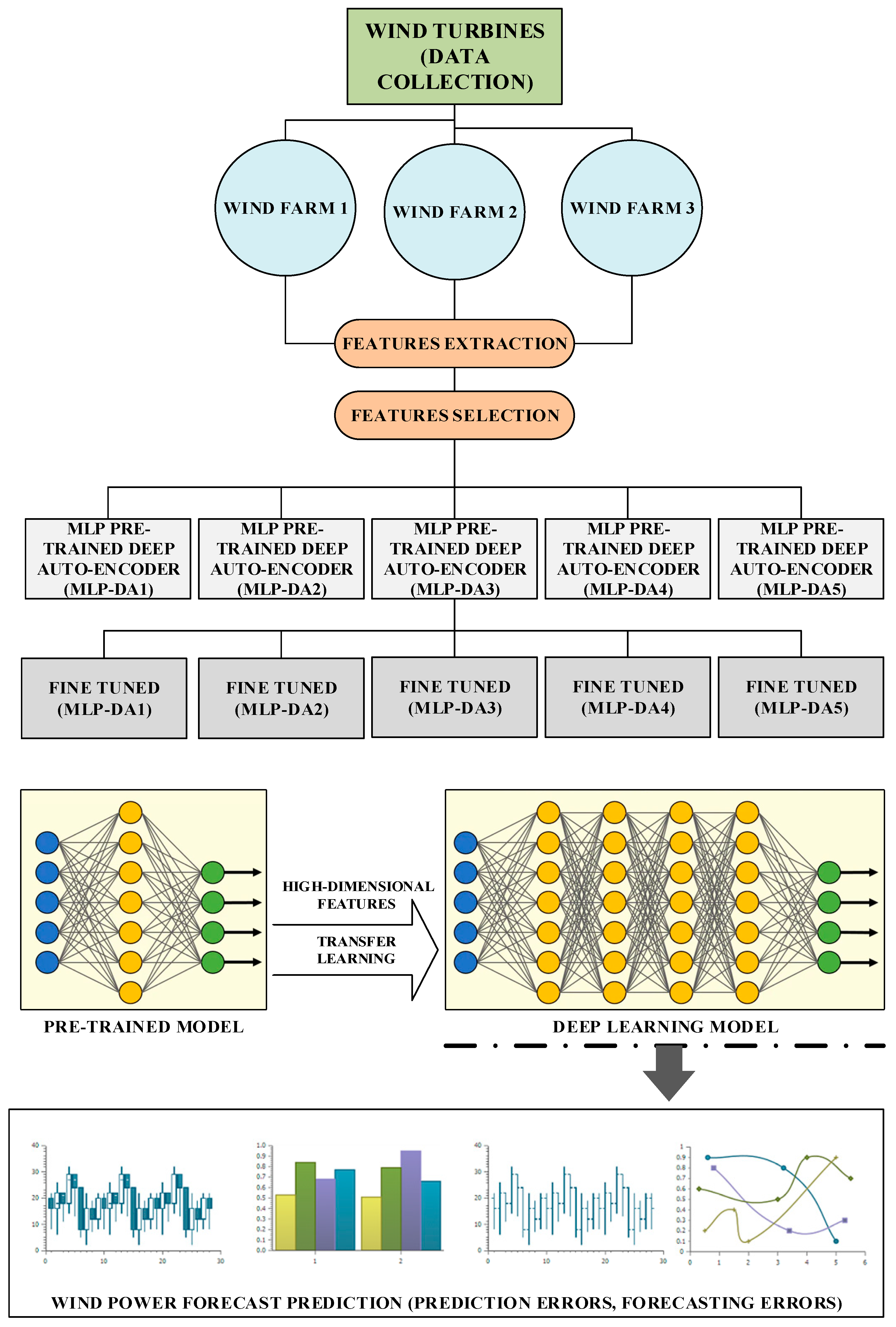
The real-time behavior of wind currents is turbulent and diverse, making wind-based power forecasting a challenging and difficult task. To analyze the impact of wind currents on power generation, raw wind power data was selected based from three windfarms located in different regions. The raw wind data was further analyzed to achieve reliable wind power forecasting. To analyze the variations in wind speed data, a set of five deep autoencoders were used to capture hidden and diverse information in low dimensional space. Deep autoencoders can enhance the forecasting accuracy and prediction time of deep learning models. The proposed forecasting model with deep autoencoders can efficiently realize encoded wind power data for reliable forecasting. In this research framework, autoencoders were used to implement dimensionality reduction on variational wind parameters to achieve optimal forecasting accuracy.

The pretrained models were further utilized for transfer learning on all three windfarms. Lastly, the forecasting accuracy for the regional wind farms was measured based on forecasting error indicators such as MAE, RMSE, etc. The overall structure of the proposed wind power forecasting model is shown in Figure 1.

3.1. MLP Deep Auto-Encoder for Dimensionality Reduction

The MLP Deep auto-encoder architecture is intended to create a representation of the input data that is as similar to the original as possible. However, the actual use of MLP deep auto-encoders is to determine a processed prototype of the input data with the least amount of data loss, which is known as dimension reduction. The encoder and decoder are key features of the MLP auto-encoder. In order to recreate the input as exactly as possible, the encoder compresses the data while the decoder generates an uncompressed version. Therefore, MLP Deep Auto-encoders typically outperform other auto-encoders due to their capacity to reassemble inputs and create identical enactments on similar datasets, resulting in distinctive parameter configurations.

Additionally, two auto-encoders and the Softmax activation function are used in the MLP deep auto-encoder. The auto-encoders learn high-dimensional data from the input vectors while also reducing the number of attributes. In contrast, rapidly decreasing the variety of features in one auto-encoder might result in critical features being missed and accuracy being negatively impacted. A typical MLP auto-encoder classifier discriminates against the hidden layer on multiple levels, including nonlinear stimulation, to differentiate nonlinear differentiated data [43]. Firstly, the encoding strategy can use the encoding function to encode the assigned input, as shown in Equation (1).

$$h=f(W_1\stackrel{-}{x}+b)$$

(1)

where the weight matrix is denoted by W₁, and the bias vector by b. Secondly, the decoding method can decode the encoded function and recreate the actual input, as indicated in Equation (2).

$$\stackrel{\wedge }{x}=g(W_{2}h+c)$$

(2)

where W₂ is the weight matrix, c is the bias vector, and g(.) is the sigmoid function. MLP Auto-encoders are also used to identify optimal parameters throughout the training phase by minimizing the squared reconstruction error, as represented in Equation (3).

$$L(x,\stackrel{\sim }{x})={\displaystyle \sum _{i=1}^n\parallel x_i-}\stackrel{\wedge }{x_i}{\parallel }^2$$

(3)

The main characteristics of the presented MLP auto-encoding method are as follows:

-

MLP Auto-encoders can only compress data in an effective manner if that data is similar to the data they were trained on.

-

MLP Auto-encoders do not require explicit labels to train, and instead, create their own labels from the training data; therefore, they are classified as unsupervised learning approaches.

-

They outperform principal component analysis techniques in terms of dimensionality reduction by presenting data as nonlinear representations, and are well suited for the extraction of features.

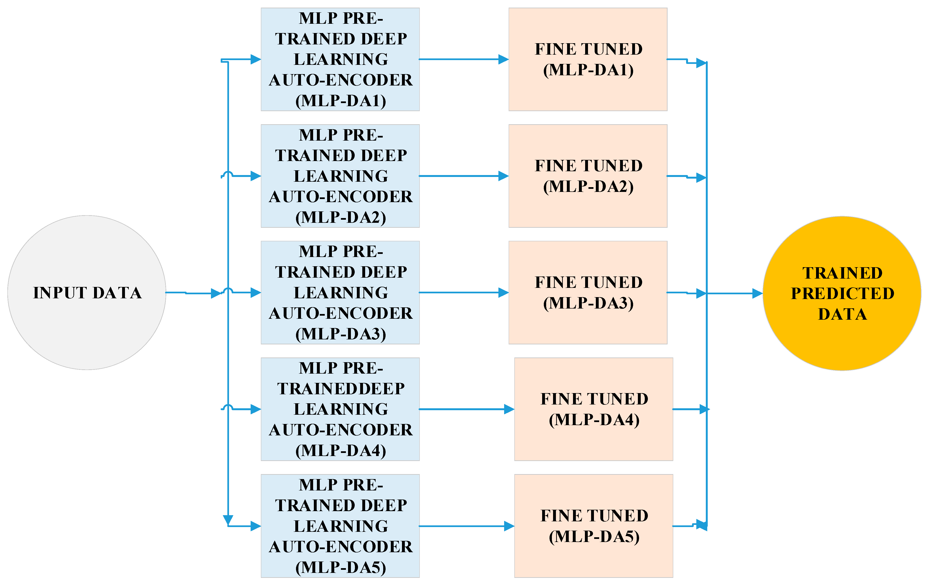
Effective power forecasting is a challenging task, because wind currents are unreliable and uncertain. Wind turbulence generates a huge amount of training data, which has a tremendous influence on the accuracy of wind power forecasting. In our model, firstly, hidden features and significant data trends were extracted in a low-dimensional region in all three windfarm datasets using a collection of five MLP deep auto-encoders. A computation diagram of the presented MLP-based Deep Auto-Encoding system is presented in Figure 2. In the proposed auto-encoder scheme, the dimension reduction method was selected for windfarm datasets to enhance the effectiveness of wind power forecasting, especially for transfer learning.

3.2. Windfarm (NREL) Dataset

Windfarm datasets are preprocessed based on the U.S. NREL repository from different regions. The collected datasets provide wind and energy measurements from different wind turbines from three different regions under certain intervals. The first regional dataset comprised a 20–160 m surface area along with time-series measurements with durations of 1 h, 7 h and 12 h. The second dataset was for Hawaii, with an average surface area of 2 km. The dataset contained wind and power measurements collected in the month of January. The third dataset consisted of an offshore region, containing different wind speed and generated power parameters. The wind speed (m/s) dataset consisted of time-series measurements spanning 17 years with various meteorological specifications collected by Modern-Era Retrospective Analysis (MERRA-1).

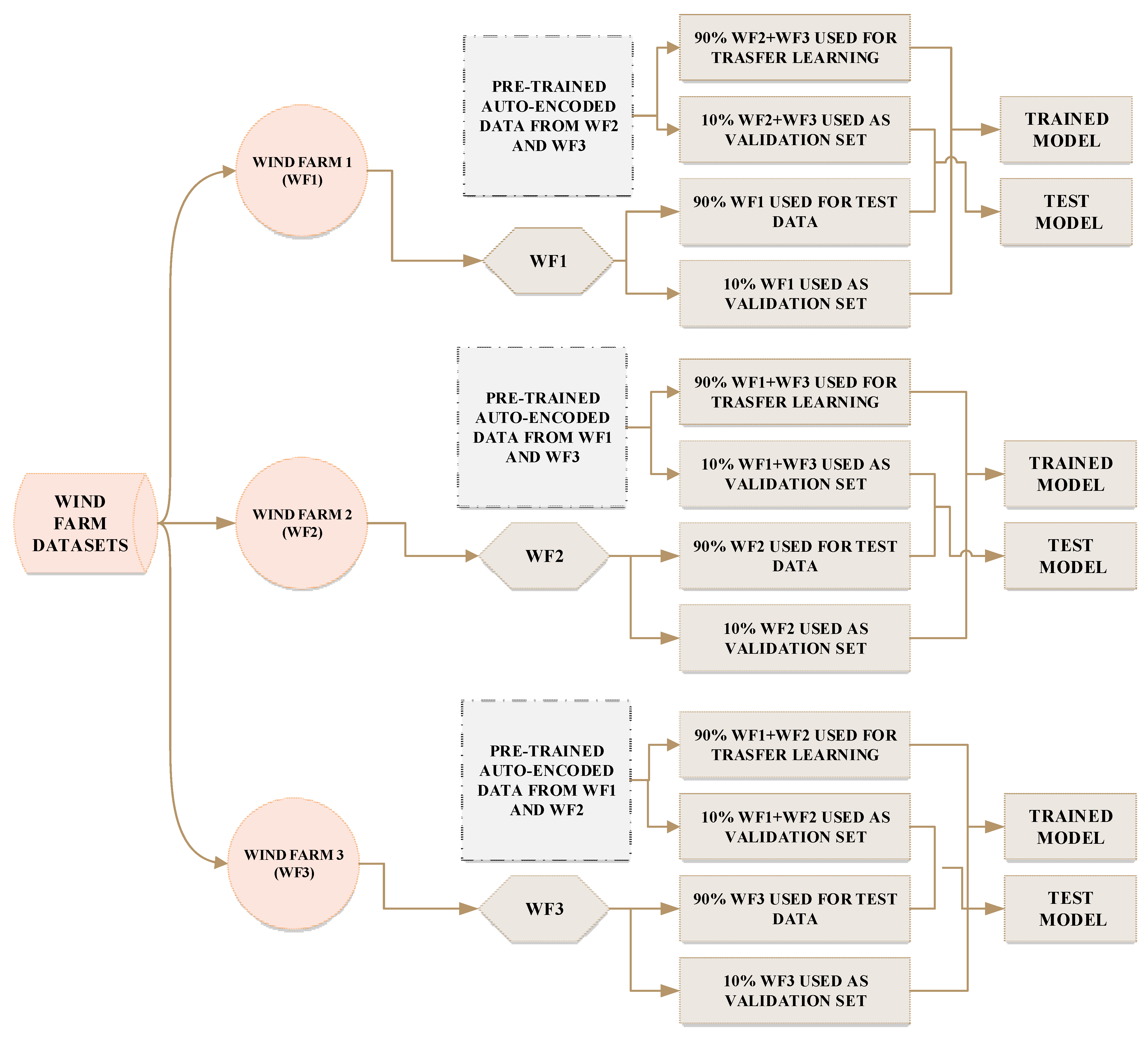
Figure 3 demonstrates the division of the datasets for all three windfarms. Three windfarm datasets were assessed to measure the effectiveness of the proposed forecasting model. Data were separated according to a certain distribution for the testing and training of each windfarm dataset. Our proposed framework comprises three phases.

In the first phase, the training of Windfarm 1 (WF1) was performed using data from the second and third windfarms. In the second phase, the training of Windfarm 2 (WF2) was performed using data from the first and third windfarms. In the third phase, the training of Windfarm 3 (WF3) was performed using data from windfarms 1 and 2. Throughout the first phase, 90% of the data (WF2 + WF3) was reserved for transfer learning, where 90% of WF1 data was used for testing purposes. The remaining 10% of WF2 + WF3 and WF1 data were used for validation purposes. During the second phase, 90% of data (WF1 + WF3) was reserved for transfer learning, while 90% of WF2 data was used for testing purposes. The remaining 10% of WF1 + WF3 and WF2 was used for validation purposes. During the third phase, 90% of data (WF1 + WF2) was reserved for transfer learning, while 90% of WF3 data was used for testing purposes. The remaining 10% of WF1 + WF2 and WF3 was used for validation purposes. Lastly, all data (WF1, WF2, WF3) from the three windfarms were used to train the model regarding selected parameters during the validation phase.

3.3. Deep Learning via Transfer Learning with TensorFlow Framework

To apply our transfer learning scheme, the pretrained model was utilized for the deep neural network in order. TensorFlow is a widely used and accessible repository for AI that works in a variety of diverse and complex environments. It has been used in high-performance computing, big data training, and state-sharing operations to mutate workflow graphs involving calculations across each neural network. TensorFlow can also acquire data nodes from a cluster spanning many processors, such as the Multicore CPU, the GPU, and a broad range of computing devices. TensorFlow allows application developers to develop various forms of reasoning applications for the design of effective deep learning models. Deep learning models usually work in three phases: the initial phase is related to data analysis; the next phase is related to architecture design; and the last phase is related to model training and evaluation. TensorFlow performs operations in the form of multidimensional arrays, also known as tensors. Tensors are different types of data forms used to generalize vectors and data metrices. They further define the distinct attributes of physical systems, and are computed simultaneously using the feature queues provided by the TensorFlow framework [44,45]. TensorFlow has been used to build complicated neural networks for forecasting models with the Keras Application Programming Interface (API) in the training of models for deep learning. 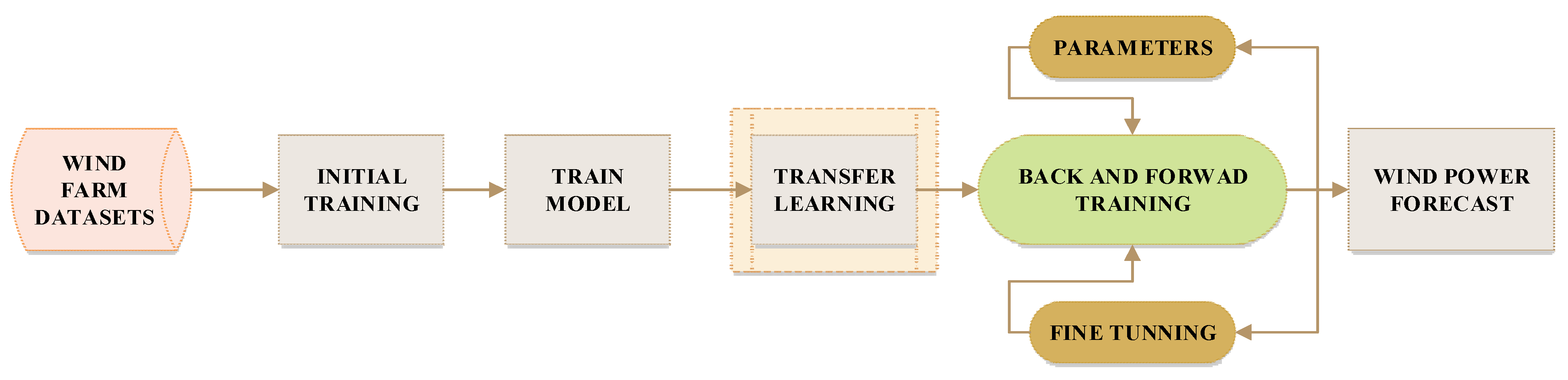Keras is an easy-to-use API for basic tooling, prototyping, as well as for modular extensions [46]. The preprocessed data are provided as input to the TensorFlow framework before model training and validation of test data via wind power forecasting, as shown in Figure 4. Input data are first trained from another model, and transfer learning is applied to train using the data prior to the actual wind power forecasting.

In a TensorFlow framework, the fine-tuned parameters are enforced based on various built-in configurations such as activation function, drop-out layer, loss feature, optimization, learning ratio (percentage), etc. Fine-tuned configurations can also increase the prediction accuracy for wind energy. The selected input variables of the windfarm datasets were “Capacity”, “Used Area”, “Grid ID”, and “Wind Speed”, and the output variable was “Wind Power”. For each windfarm dataset, the optimal fine-tuned configurations are given in

Table 1. The optimal fine-tuned configuration selected for Windfarm 1.

Layer ID	No. of Neurons	Maximum Epoch	L2 Weight Regularization	Dropout Ratio
1	200	400	0.00002	0.2
2	175	350	0.00001	0.1
3	150	300	0.00001	0.1
4	100	250	0.00001	0.1
5	70	200	0.00001	0.1

,

Table 2. The optimal fine-tuned configuration selected for Windfarm 2.

Layer	No. of Neurons	Maximum Epoch	L2 Weight Regularization	Dropout Ratio
1	250	400	0.00003	0.2
2	200	400	0.00001	0.2
3	175	350	0.00001	0.1
4	150	300	0.00001	0.1
5	100	250	0.00001	0.1
6	90	200	0.00002	0.1
7	60	200	0.00002	0.1

and

Table 3. The optimal fine-tuned configuration selected for Windfarm 3.

Layer	No. of Neurons	Maximum Epoch	L2 Weight Regularization	Dropout Ratio
1	250	400	0.00003	0.2
2	200	350	0.00001	0.2
3	175	300	0.00001	0.1
4	150	300	0.00001	0.1
5	100	250	0.00001	0.1
6	90	200	0.00002	0.1
7	60	200	0.00002	0.1
8	50	200	0.00002	0.1

, respectively. The number of neurons for hidden layers varied between 50 to 250, and the size of the epochs varied between 200 to 400. The collected datasets were pretrained after preprocessing with deep autoencoding and saved as trained models. The pretrained model was further analyzed and integrated in the proposed deep learning framework via a transfer learning scheme. Finally, wind power was predicted for all three windfarm regions. In the case of the input layer, the Rectified Linear Unit (ReLU) activation function was implemented. In deep neural networks, the ReLU activation function is widely used by researchers due to its high efficiency. The ReLU activation function is numerically represented in Equation (4).

$$f(x)=x^{+}=\max (0,x)$$

(4)

where $x$ represents the input data for the neural network, which is also a ramp function.

In the proposed deep learning model, the Softmax method was used as an activation function to evaluate forecasting errors. The Softmax algorithm generalizes the multidimensional logistic equation and effectively works with regression analysis. Additionally, it function stabilizes the performance distribution probability with the expected outputs [47]. Our neural network used the Softmax function to normalize the outputs based on the transformation of weights into the sum of probabilities. The Softmax function interpreted the probability of the expected output using Equation (5).

$$\sigma {(\overrightarrow{z})}_i=\frac{e^{z_i}}{{\displaystyle {\sum }_{j=1}^K{e}^{z_j}}}$$

(5)

where $\sigma$ signifies the Softmax function, $\overrightarrow{z}$ is the input vector, and $e^{z_i}$ is an exponent for the given vector. In deep learning, the entropy function is often used to evaluate forecasting losses such as accuracy and validation loss. An optimizer function may be used to minimize error and optimize the accuracy of deep learning models. We selected the Adam optimizer to configure the proposed forecasting model; this optimizer operates by modifying weights for active learning in deep learning architectures [48]. A regularization strategy decaying mean is often applied to neural network weights for the generalization and optimization of training models using, for example, Equations (6) and (7) [49].

$$m_t={\beta }_1{m}_{t-1}+(1-{\beta }_1)g_t$$

(6)

$$v_t={\beta }_2{v}_{t-1}+(1-{\beta }_2)g_t{}^2$$

(7)

where $m_t$ and $v_t$ are used as approximate measures, also known and the first and second moments of weight decay for each gradient. Parameters ${\beta }_1$ and ${\beta }_2$ measure how quickly the averages decay over the gradient squared $g_t{}^2$. As optimizer algorithms use moving averages which tend to be biased, an extra step is required for bias correction. The Adam optimizer measures bias-corrected moments utilizing Equations (8) and (9), where ${\widehat{m}}_t$ is the bias-corrected first moment and ${\widehat{v}}_t$ is the bias-corrected second moment.

$$\stackrel{\wedge }{m_t}=\frac{m_t}{1-{\beta }_1^t}$$

(8)

$$\stackrel{\wedge }{v_t}=\frac{v_t}{1-{\beta }_2^t}$$

(9)

The cross-entropy function utilizes wind power forecasting losses and errors. We selected sparse categorical cross-entropy as a loss function, which transformed targeted output into categorical formats [50]. When the actual labels for forecasting were numbers such as generated wind power, the sparse categorical cross-entropy function was shown to be more effective. The loss function model was mathematically measured using Equation (10).

$$J(w)=-\frac{1}{N}{\displaystyle \sum _{i=1}^N[y_i\log ({\widehat{y}}_i)+(1-y_i)\log (1-}{\widehat{y}}_i)]$$

(10)

where neural networks weights are represented by w, the actual labels of validation data are represented by $y_i$ and the predicted labels are represented by ${\widehat{y}}_i$.

4. Results and Discussion

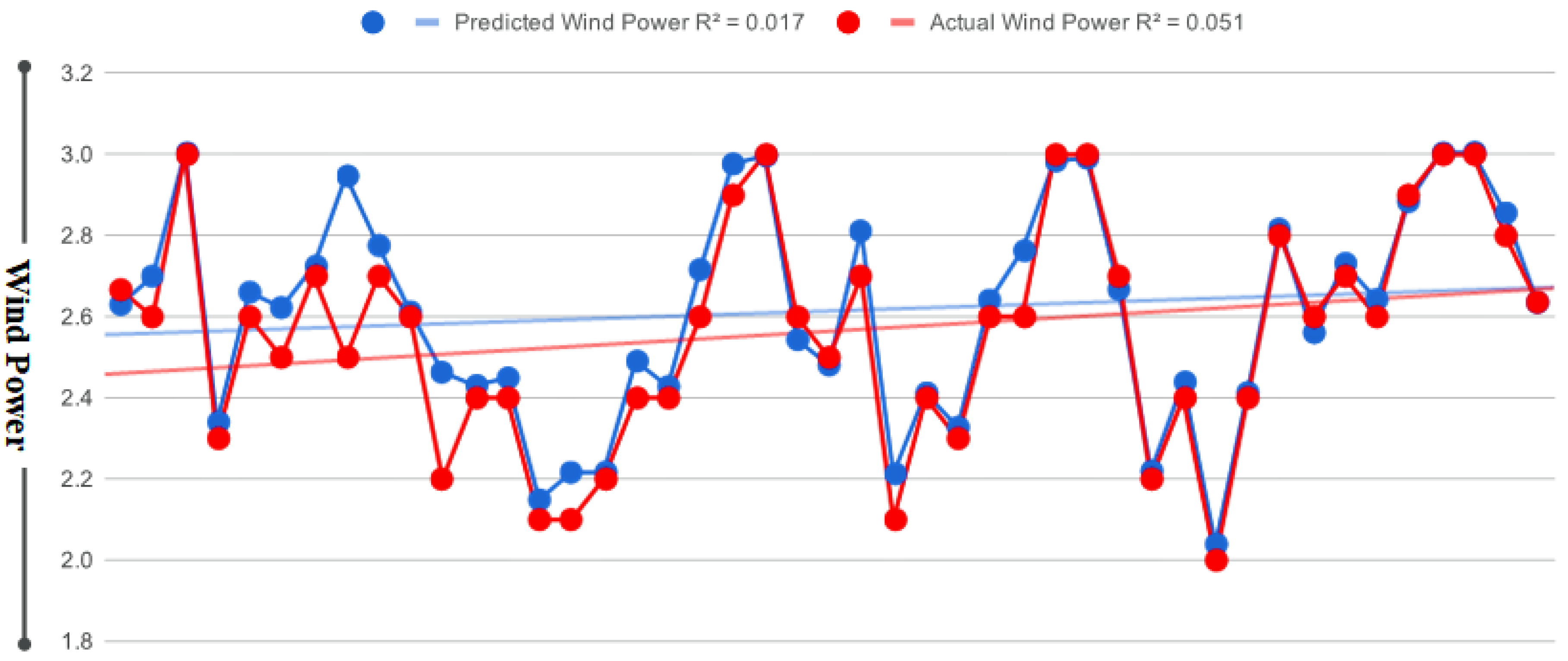
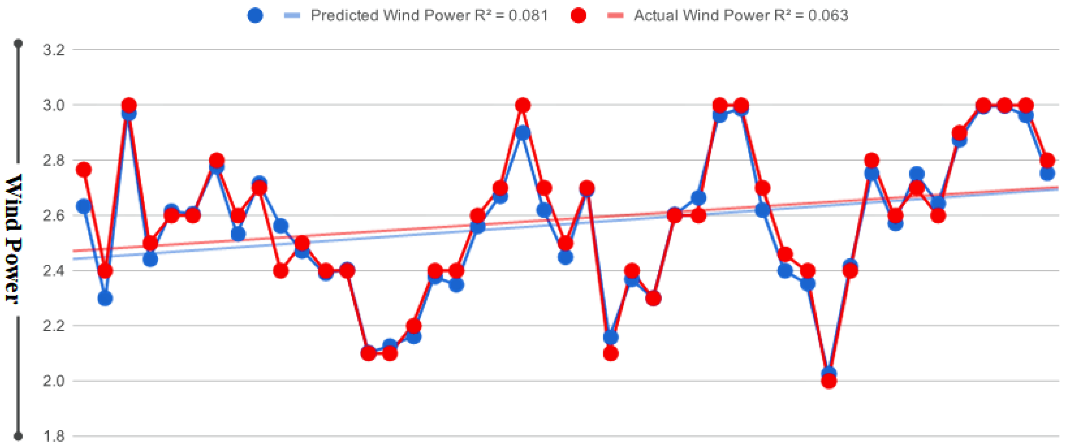
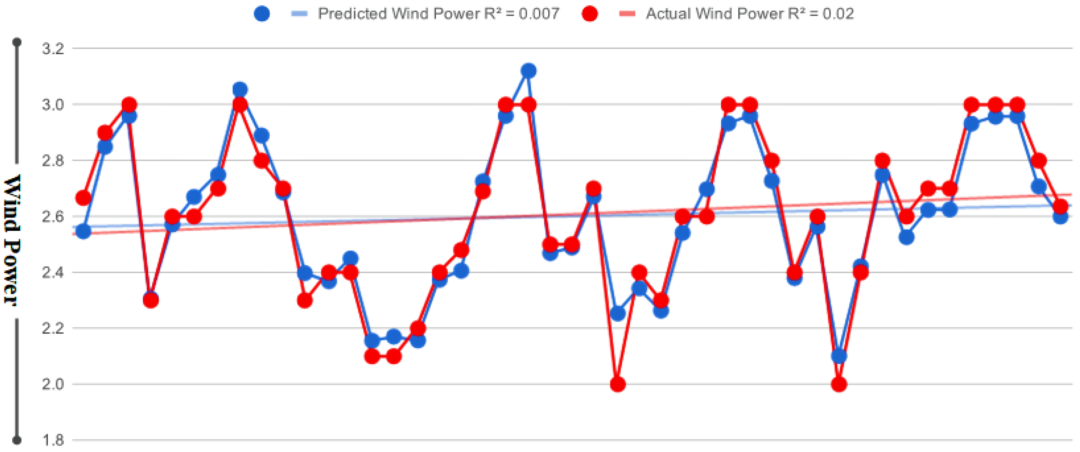
The Keras interface provides an easy way to transform different layers and functions in the TensorFlow platform for the design of forecasting models [51]. The user-defined functionality can perform complex forecasting tasks in short periods of time. The proposed forecasting model was compiled for each windfarm. The actual and predicted wind power outcomes for each dataset are shown in Figure 5, Figure 6 and Figure 7, respectively. Figure 5 shows the proximity between the original and forecasted outcomes and their R-squared correlation for Windfarm 1, Figure 6 shows the actual and forecasted outcomes linked to Windfarm 2, and Figure 7 shows the forecasted outcomes related to Windfarm 3. In each figure, the blue curve indicates the predicted power outcomes, while the red curve shows the original power outcomes generated by the windfarms at different intervals. All figures show that the predicted and actual wind power is closely related, with only minor variations. The forecasting assessment therefore revealed that the proposed forecasting model is very effective for forecasting wind energy, while transfer learning is more suitable for improving forecasting outcomes with less training on large and complex regional windfarms.

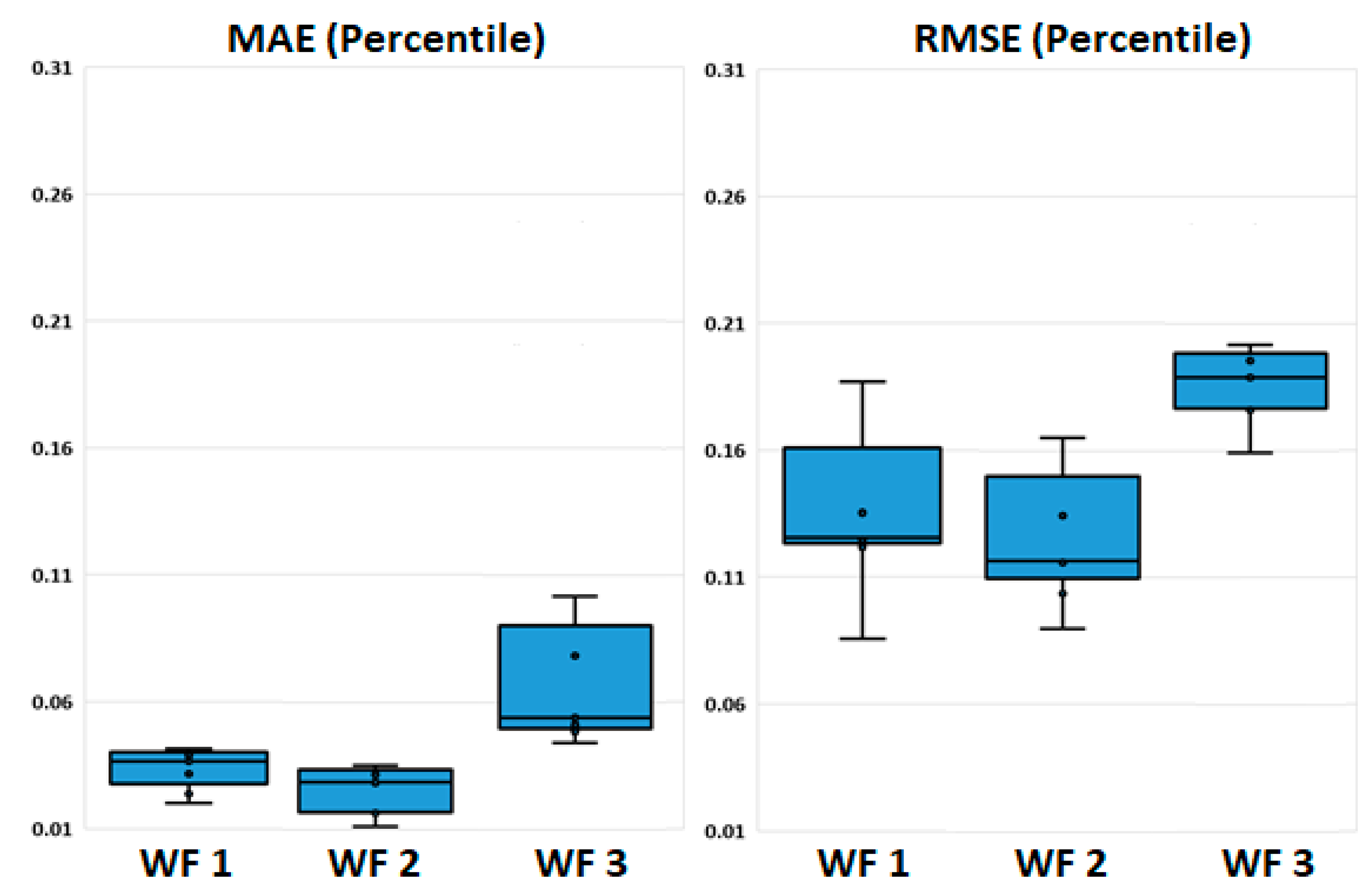
The forecasting accuracy was further analyzed based on forecasting errors such as MAE and RMSE. The lower error suggests that the proposed model can effectively forecasts wind energy, while higher error rates suggest that the model is ineffective in its current form. Figure 8 shows the percentile distribution of MAE and RMSE errors for all three windfarms. The lowest MAE range for windfarms was between 0.01 and 0.10, while the lowest RMSE range was between 0.08 and 0.20. The MAE and RMSE assessments indicated that the methods proposed in this study are quite effective for regional windfarms. A lower error percentile indicates a higher degree of confidence and higher accuracy.

The proposed forecasting model utilized optimal fine-tuned parameters such as activation, optimization, and loss functions [52] to calculate MAE and RMSE errors. The obtained MAE and RMSE values for Windfarm 1 ranged between 0.02 and 0.0858, for Windfarm 2 between 0.0111 and 0.0899, and for Windfarm 3 between 0.0443 and 0.1594. Equations (11) and (12) were used to calculate the MAE and RMSE errors, especially for the forecasting of timeseries data [53,54].

$$\mathrm{MAE}=\frac{{\displaystyle {\displaystyle \sum }_{i=1}^n}|y_i-x_i|}{n}$$

(11)

where $y$ is the forecasted variable, $x$ is the original variable, and $n$ is the number of observations in each windfarm. The cumulative variations between the forecasted and original variables were measured in terms of RMSE using the following equation:

$$\mathrm{RMSE}=\sqrt{\frac{{\displaystyle {\displaystyle \sum }_{t=1}^T}{\left(x_{1,t}-x_{2,t}\right)}^2}{T}}$$

(12)

Whenever the expected value was $x_{1,t}$, $x_{2,t}$ is the observed value and $T$ represented the cumulative number of observations. The forecasted MAE and RMSE errors of the proposed models were further compared with the state-of-the-art models listed in

Table 4. Comparison of related forecasting models with the proposed model in terms of MAE and RMSE forecasting errors for windfarms.

Dataset	Errors	RF	J48	RT	SVM	ES	BPNN	RNN	LSTM	PM
WF 1	MAE	0.0389	0.0415	0.0237	0.2257	0.0366	0.0317	0.0250	0.0182	0.0200
	RMSE	0.1245	0.1868	0.1353	0.2817	0.1256	0.1218	0.1073	0.0851	0.0858
WF 2	MAE	0.0165	0.0285	0.0173	0.2246	0.0353	0.0316	0.0180	0.0173	0.0111
	RMSE	0.1038	0.1653	0.1166	0.2734	0.1344	0.1160	0.1102	0.0902	0.0899
WF 3	MAE	0.1020	0.0486	0.0512	0.2336	0.0540	0.0785	0.0914	0.0425	0.0443
	RMSE	0.1772	0.2018	0.1889	0.2891	0.1761	0.1954	0.1671	0.0161	0.1594

Note: WF = Windfarm, RF = Random Forest, RT = Regression Tree, ES = Ensemble Selection, PM = Proposed Method.

. The overall accuracy of the proposed model was better than those of the other models, i.e., between 0.0111 and 0.1594. Windfarm 2 achieved the lowest MAE and RMSE errors in our model. In the case of Windfarm 3, the MAE and RMSE were also less than 5% and 16%, respectively. However, the LSTM model achieved the lowest MAE and RMSE on the Windfarm 1 dataset. One possible reason for this is that LSTM models tend to perform better for short-term forecasting. However, the overall performance of the proposed method was far better than those of other state-of-the-art models. Apart from that, the Random Forest showed good accuracy with an MAE value of 0.0165 and an RMSE value of 0.1038 for Windfarm 2. Other forecasting models such as RNN, J48 and ensemble selection showed MAE and RMSE values between 0.486 and 0.1761, showing the effectiveness of variational autoencoding in terms of power forecasting.

The MAE and RMSE values were further normalized to compare forecasting errors under different scales such as NMAE and NRMSE. The NRMSE metric can be used to validate the reliability of forecasting models. The normalized NMAE and NRMSE values for the proposed and other models are shown in

Table 5. Comparison of related forecasting models with the proposed model in terms of Normalized MAE and RMSE forecasting errors.

Dataset	Errors	RF	J48	RT	SVM	ES	BPNN	RNN	LSTM	PM
WF 1	MAE	0.0070	0.0058	0.0041	0.0354	0.0061	0.0053	0.0035	0.0028	0.0030
	RMSE	0.0221	0.0316	0.0215	0.0443	0.021	0.0185	0.0142	0.0116	0.0127
WF 2	MAE	0.0019	0.0032	0.0021	0.0317	0.0045	0.0035	0.0017	0.0014	0.0012
	RMSE	0.0153	0.0235	0.018	0.0372	0.0189	0.0146	0.0135	0.0117	0.0115
WF 3	MAE	0.0124	0.0064	0.0066	0.0316	0.0316	0.0102	0.0074	0.0052	0.0046
	RMSE	0.0233	0.0259	0.0240	0.0371	0.0234	0.0247	0.0312	0.0231	0.0201

Note: WF = Windfarm, RF = Random Forest, RT = Regression Tree, ES = Ensemble Selection, PM = Proposed Method.

. The normalized MAE and RMSE values also showed the reliability of our forecasting model, achieving NMAE and NRMSE values between (0.0030, 0.0127), (0.0012, 0.0115), (0.0046, 0.0201) for the Windfarms 1, 2, and 3, respectively.

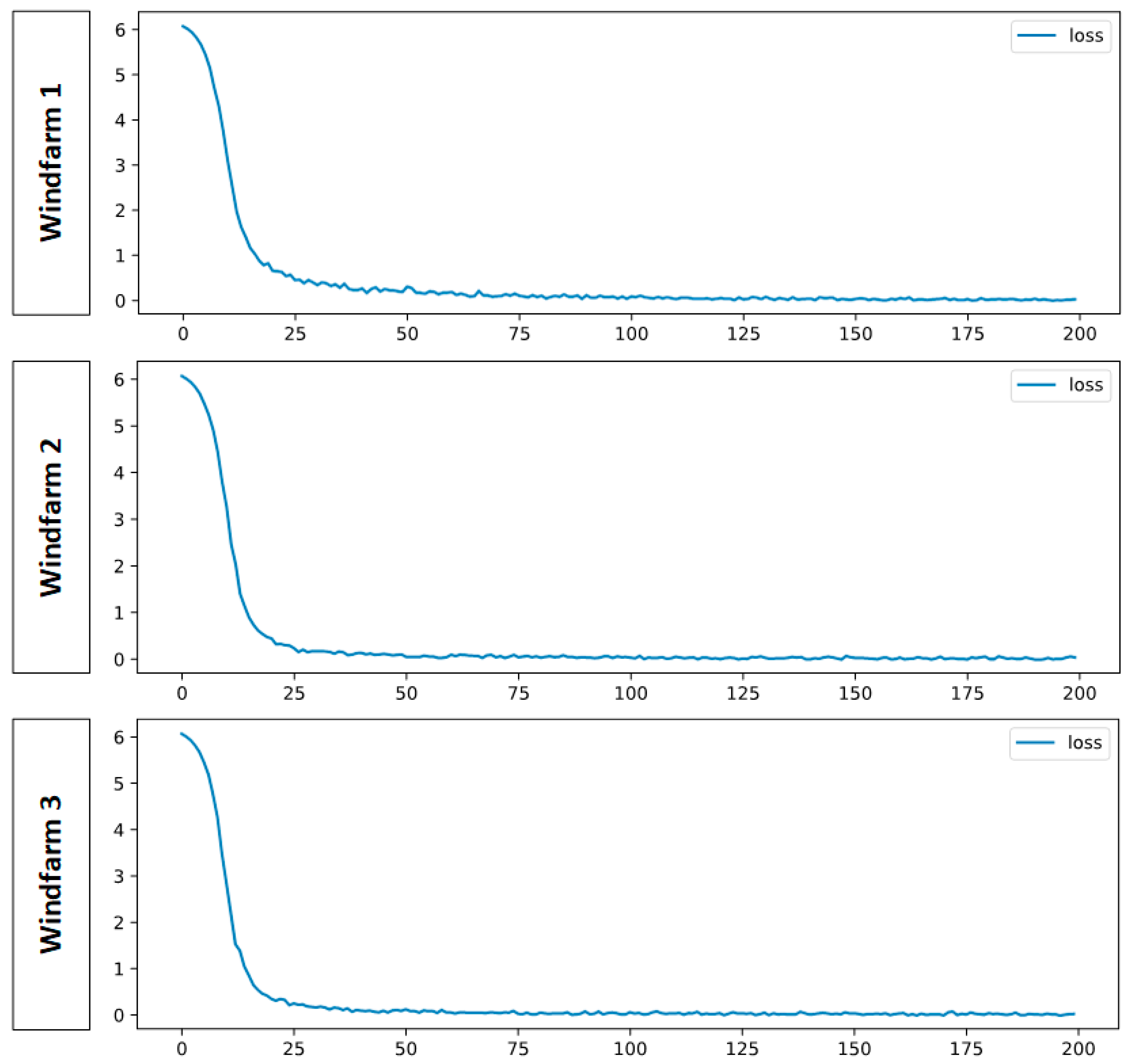
Deep learning models often under- or over- fit, depending on the data and fine-tuned parameters. Thus, retraining errors were visualized via epochs to measure the stability and feasibility of the deep learning model for wind power data and the fine-tuned parameters. In this study, the proposed deep learning model was executed against 200 epochs on three windfarm datasets to validate its stability and measure retraining losses. Figure 9 shows the retraining loss produced by proposed model, where the x-axis represents loss against the next epoch cycle and the y-axis represents the accuracy loss for each windfarm.

As shown in Figure 9, the training error was close to 60% in the first epoch cycle. However, with every subsequent cycle, the training error continued to decrease and the accuracy of the model improved, which shows the stability of the proposed strategies for wind power data without any under- or over- fitting of the deep learning model. The retraining loss was lowest between 25 to 50 epochs and remained stable for the remainder of the epochs. For instance, the retraining loss was less than 5% after 50 epochs, and remained between 1% to 2% on subsequent epochs. In conclusion, Figure 10 illustrates that our neural network model is suitable for forecasting wind power using a given dataset, that a minimum of 50 epochs is required to consistently achieve accuracy, and that a minimum error of between 1% to 5% is generated by the forecasting model. The training loss was measured by fitting training and validation data as a linear curve. The slight variation in the linear curve indicated the suitability of variational auto-encoders and hybrid transfer learning for wind power forecasting.

Table 6. Runtime Comparison before and after using Auto-Encoder + Hybrid Transferred Learning.

Dataset	Errors	RF
Wind Farm 1	35.18 s	8.12 s (76.91×)
Wind Farm 2	19.02 s	6.85 s (63.98×)
Wind Farm 3	11 m 10 s	2 m 41 s (75.97×)
Auto-Encoder + Hybrid Transferred Learning		Average (72.29×)

provides a runtime comparison of the proposed and other methods using all three datasets. Windfarms 1 and 3 shortened the model training runtime by more than 75× while preserving high accuracy. Windfarm 2 yielded the least runtime reduction, which was nonetheless more than 63×, proving the feasibility and effectiveness of the proposed solutions. All experiments were performed on a system with a 6 Core i7-8750H 2.20 GHz processor, 16 GB RAM and GTX1060 6G Nvidia GPU. Python 3.8 64-Bit version and Visual Studio 2017 SDK were used to implement the wind power forecasting methods.

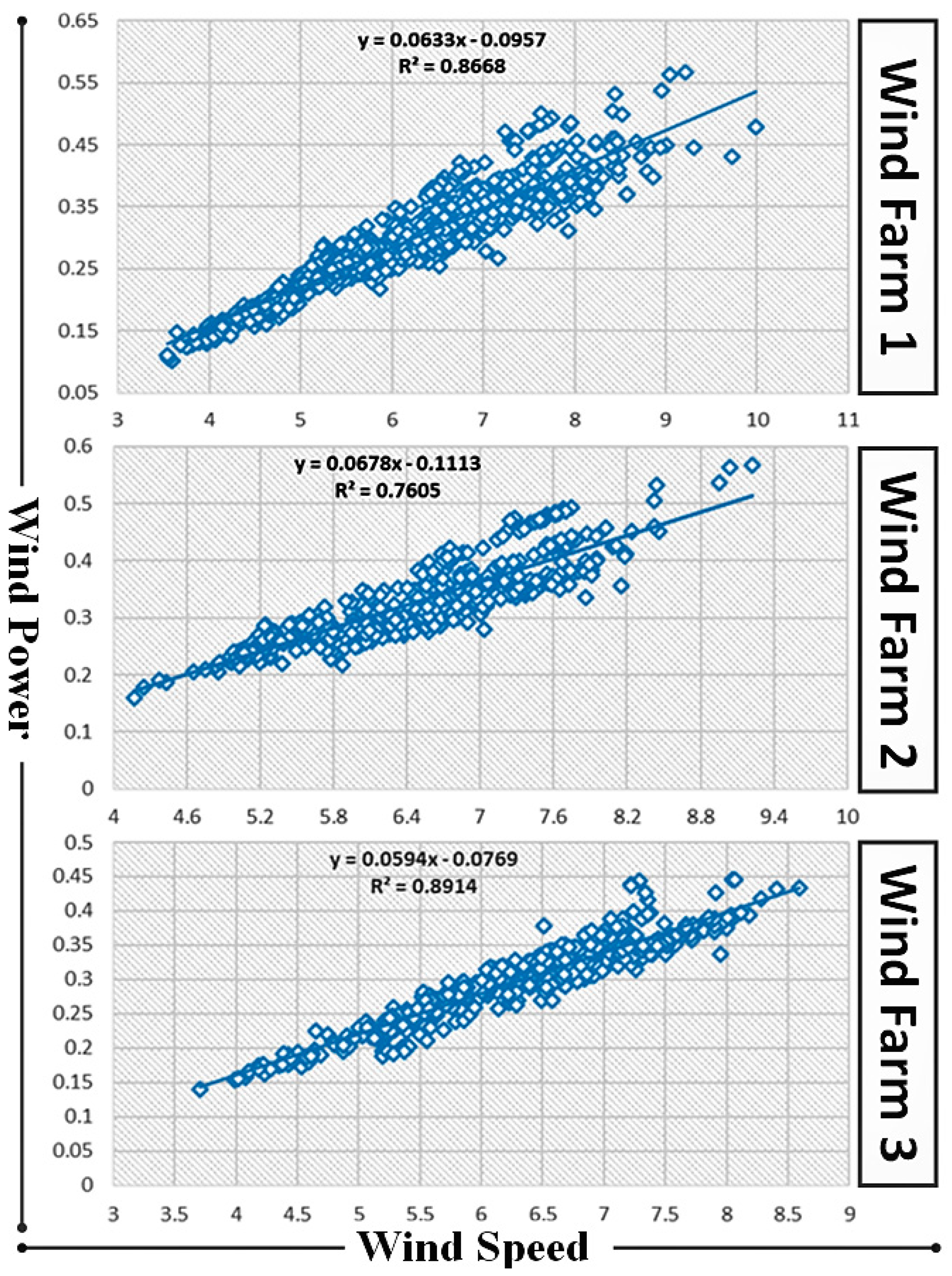
In the final experiment, wind characteristics such as speed and power were linearly fitted on the x- and y-axes via r-squared correlation. The association between speed and power explained the suitability of the forecasting model for the selected wind power data. High association indicated a high degree of dependency of different variables on each other. Figure 10 shows the linear association of wind power and speed variables for all three windfarms. The data points are plotted in blue dots and the linear regression line was determined using the fit equation. Data points which are close to each other indicate a high degree of association between two variables. The r-squared correlation for the three windfarms was 86.68%, 76.05% and 89.14%, respectively, indicating the suitability of wind characteristics for power forecasting. As shown in Figure 10, the data points of Windfarm 3 were more proportionate to the linear regression line compared to those of the other two datasets. As a consequence, the r-squared correlation of Windfarm 3 was higher than those of Windfarms 1 and 2.

5. Conclusions

A novel strategy to forecast wind power with the aid of variational auto-encoders and transfer learning was designed for massive and multiregional windfarms. The proposed forecasting model was applied to three windfarm datasets from different regions. Although the power densities of the three sites varied, the principle of transfer learning was shown to effectively and swiftly predict wind power. Therefore, the raw information from the selected regions was screened, and variables with high associations with power production were selected. Variational auto-encoders were used for backpropagation neural network training in order to distinguish data that were not linearly separable. Transfer learning showed that one windfarm could be fine-tuned to forecast wind power for other regions with similar characteristics. As a result, the computational cost of retraining data was reduced by 90×. The minimum MAE and RMSE ratios estimated using the proposed model were 0.0111 and 0.0858, while the maxima were 0.0443 and 0.1594, respectively. The lower computational cost and reduced error ratios suggest that the proposed method can efficiently forecast wind power, regardless of multiregional physical attributes.

In future, we intend to use the proposed methods for short-term power forecasting. Since short-term meteorological data typically consist of minute and hourly energy output, there is a high possibility that transfer learning may influence predictive outcomes. To overcome this, optimization and data dimensionality reduction methods will be adopted.