Machine Learning Models for Early Prediction of Sepsis on Large Healthcare Datasets

Abstract

Sepsis is a highly lethal syndrome with heterogeneous clinical manifestation that can be hard to identify and treat. Early diagnosis and appropriate treatment are critical to reduce mortality and promote survival in suspected cases and improve the outcomes. Several screening prediction systems have been proposed for evaluating the early detection of patient deterioration, but the efficacy is still limited at individual level. The increasing amount and the versatility of healthcare data suggest implementing machine learning techniques to develop models for predicting sepsis. This work presents an experimental study of some machine-learning-based models for sepsis prediction considering vital signs, laboratory test results, and demographics using Medical Information Mart for Intensive Care III (MIMIC-III) (v1.4), a publicly available dataset. The experimental results demonstrate an overall higher performance of machine learning models over the commonly used Sequential Organ Failure Assessment (SOFA) and Quick SOFA (qSOFA) scoring systems at the time of sepsis onset.

1. Introduction

The most recent definition of sepsis defines the syndrome as a “life-threatening organ dysfunction due to a dysregulated host response to infection” [1,2]. Sepsis is a highly complex and heterogeneous syndrome, which is influenced by two types of characteristics: those associated with the patient (e.g., immunologic status, age, comorbidities) [3,4], and those associated with the infection (e.g., site of infection, pathogen type, virulence) [1,5]. As a consequence, their relative contribution to organ damage may vary across patients due to the combinations of such characteristics: sepsis is a common pathway from infection to death. Kidneys, liver, lungs, heart, the central nervous system, and the hematologic system are among the most commonly affected [2].

Management is a major challenge for healthcare systems, affecting high- and low-income countries alike [6]. Sepsis continues to be a leading cause of death worldwide; in 2017, there were an estimated 48.9 million cases and 11 million sepsis-related deaths worldwide [7]. Globally, it is associated with a 10–20% in-hospital mortality rate [2,8,9,10]. Sepsis can also be very expensive to treat, the costs for sepsis management in U.S. hospitals rank highest among admissions for all disease states, amounting to over USD 20 billion in 2011, growing to over USD 23 billion in 2013, and cost more than USD 24 billion annually [9,11,12,13].

Various investigations have demonstrated that early diagnosis and appropriate antibiotic therapy have the potential to reduce mortality among the septic population [14,15,16]. Despite this, detecting sepsis at this stage of the disease is difficult. One of the main reasons is that sepsis is a heterogeneous syndrome whose course depends on different pathophysiological mechanisms, complexity in clinical context, and clinical phenotypes. For clinicians and researchers, the challenge is to objectively assess the true magnitude of organ failure for each patient [17]. There is also a lack of accurate diagnostic tools [18]. Different and complex scoring systems have been defined for bedside evaluation, allowing early detection of patient deterioration [2,19,20]. Several scores are currently used, such as: Acute Physiology and Chronic Health Evaluation (APACHE II) [21], Simplified Acute Physiology Score (SAPS II) [22], Sequential Organ Failure Assessment (SOFA) [23], and Quick SOFA (qSOFA) [2], which have been validated to assess illness severity from the weighted combination of clinical and laboratory measures. However, these scoring systems, indeed useful for predicting general deterioration or mortality in studies conducted in intensive care units (ICU), cannot identify sepsis with high sensitivity and specificity at an individual level [2,24]. In addition, they present significant errors at patient data in clinical use, showing methodological weaknesses [25].

The accelerating generation of vast amounts of healthcare data will completely change the nature of medical care. The clinical decision support systems that integrate both laboratory data and biomarkers have the potential to greatly improve patient outcomes [26,27,28]. Assessing the utility of these complex datasets for supporting clinical decisions is the aim of most current research projects [29,30]. Recent studies have deployed ensemble models using real-world events to find important predictive parameters to track down those patients who are at the highest risk of death [31].

In the last decade, a substantial number of papers have been published on clinical applications of machine learning for the early prediction of sepsis in ICU [32,33,34,35,36,37,38,39]. However, there are important disparities in the identification of sepsis cohorts due the use of various approaches and considerable heterogeneity in definitions [30,32,40]. Many studies use ICD coding [36,41,42], which is considered an unreliable tool with limitations in identifying septic patients [43,44,45]. Others are based on systemic inflammatory response syndrome (SIRS) [37,46] or use the latest sepsis-3 criteria [47,48,49]. The major concerns regarding the clinical applicability and the actual accuracy of these models are related with the definition of sepsis, the identification of organ dysfunction, and the selection of input features [32,50,51,52,53,54,55]. By strategically deploying machine learning (ML) models and carefully selecting underlying data, cohorts, and features, algorithm developers can mitigate these concerns [51,52].

Several works used vital signs measurements and laboratory test results in order to develop models to predict sepsis during ICU stay [56,57]. Some trained ML algorithms using physiological parameters only, as input features. For example, in [49] the authors used six vital signs—heart rate (HR), respiratory rate (RR), temperature (T), peripheral oxygen saturation (SpO₂), systolic blood pressure (SBP), and diastolic blood pressure (DBP)—as the inputs in an XGBoost model. Recent studies have investigated the change in variability of vital sings with a set of the following four features: arterial pressure (AP), HR, RR and T. They developed a support vector machine (SVM) algorithm achieving a 0.88 AUC-ROC for predicting four hours before the sepsis onset [58]. Other models have added the use of laboratory test results, demographics, and comorbidities to improve the results [42,59]. In another study, a collection of six continuous minute-by-minute physiological data (HR, RR, T, $Sp{O}_2$, SBP, DBP) and the white blood cell (WBC) count were used in a random forest (RF) model with a 0.8 sensitivity within an hour before the sepsis onset [37]. In [60], the authors used 34 physiological variables, of which 5 were vitals and 29 were laboratory values in a multitask Gaussian process through a deep recurrent neural network model. Others have added the use of the six vitals, Ph, WBC, and the age to be analyzed as times series in the inSight model [41] for a 0.92 AUC-ROC.

Although there is no database with labeled sepsis cases, many studies have used the MIMIC II and MIMIC III databases. Using these databases, a wide range of prediction models have been applied for the early detection of sepsis. Some of the most prominent are artificial neural networks (ANN) [46], deep temporal convolution networks [61], deep learning (DL) models [48], RFs [37], and SVMs [58,62]. Although some of these recent efforts are promising, the lack of comparability of these studies does not allow a direct comparison [33,48]. In order to reduce this gap in a meaningful way and promote the cooperation between clinicians and researchers, the first contribution of this work is the provision of a reference database for researchers. This was developed with a detailed analysis of organs dysfunction related with sepsis patients on the MIMIC-III database.

Furthermore, this research explores the use of a proposed ML-based ensemble classification technique to develop a model for early sepsis prediction. The role of feature selection methods on the performance of the proposed ML model was investigated. To summarize, this work focuses on answering the following questions:

1.

What are the most relevant factors associated with the early prediction of ICU sepsis?

2.

Do ML techniques, especially ensemble models, outperform the current sepsis mortality scoring?

The contributions of this work are summarized as follows:

• An applicable framework is proposed for identifying sepsis onset cases in ICU for adult patients. This structured approach yields a cohort selection well suited for identifying organs dysfunction and suspected infection, following the SEPSIS-3 definition.
• An accurate and explainable sepsis prediction ensemble model is also proposed based on a comprehensive list of critical features from ICU patients. The model is based on a new ensemble algorithm using vital signs, laboratory test results, and demographics tabular variables as input. We discuss the development of different ML models, and the results are compared with the traditional scoring system.
• The effects of various feature selection methods on the identification of the relevant features for 24, 12, and 6 h observation windows were analyzed, and the results were evaluated for 1 h prediction time.

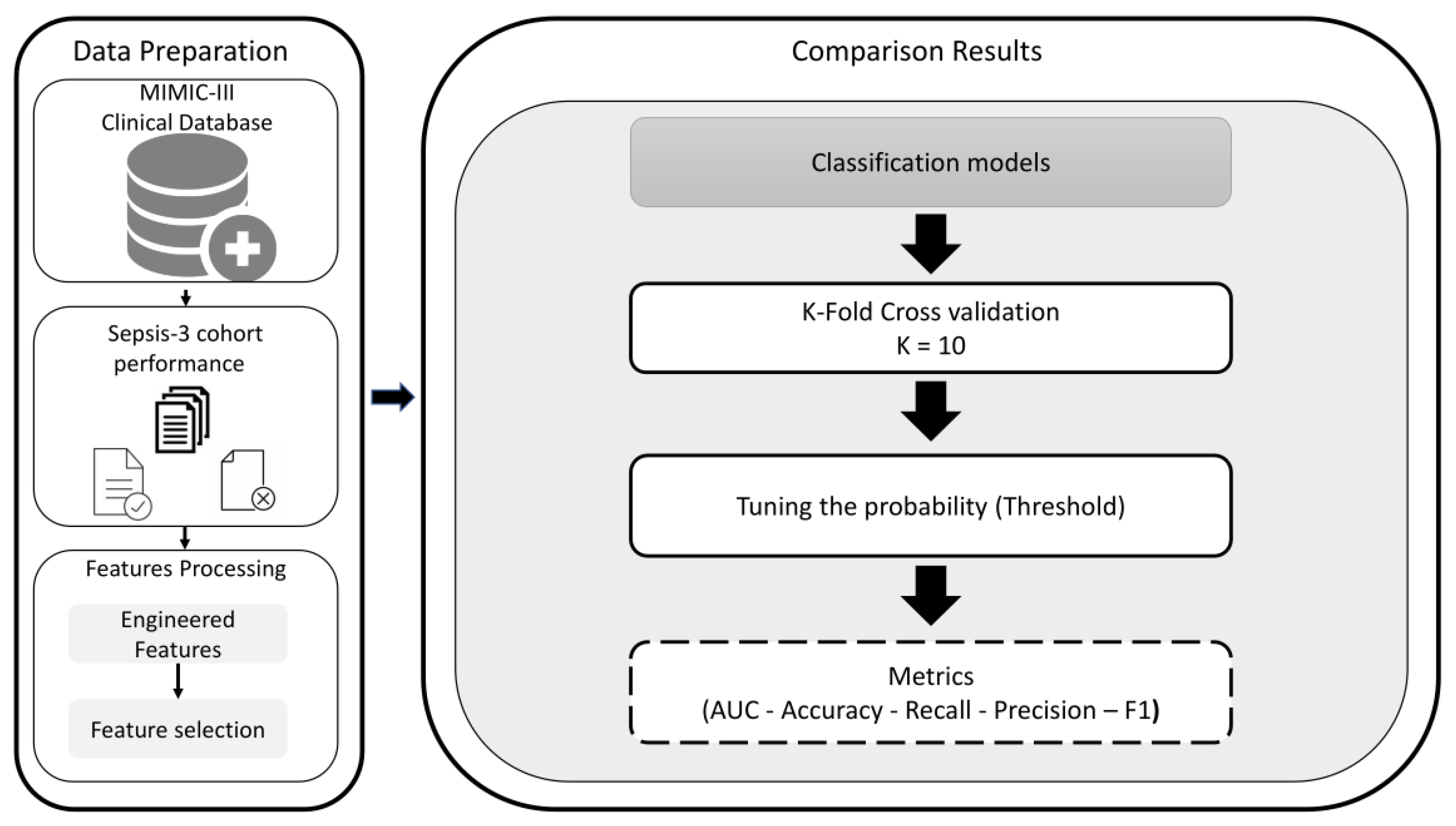
2. Materials and Methods

This section details the selected dataset, preprocessing steps, and feature selection in the experiments, following the methodology described in Figure 1.

2.1. Data Source

We used the de-identified public database MIMIC-III v1.4, which contains patient data from the Beth Israel Deaconess Medical Center (BIDMC, Boston, MA, USA) [63]. The database uses two information systems, Philips CareVue Clinical and IMDsoft MetaVision ICU, that have very different data structures. MIMIC III contains detailed information on more than 60,000 stays corresponding to more than 40,000 patients. The data are associated with 53,423 distinct hospital admissions for adult patients [64].

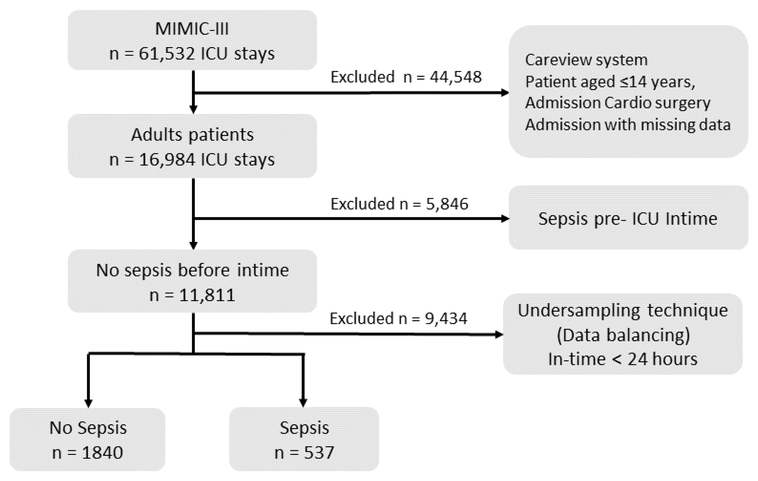
2.2. Data Selection

The aim of data preprocessing is improving the quality of the collected dataset. The data preprocessing includes selection patients cohort, data balancing, removing outliers, and handling missing data. Figure 2 details the number of patients in each step and the exclusion steps performed.

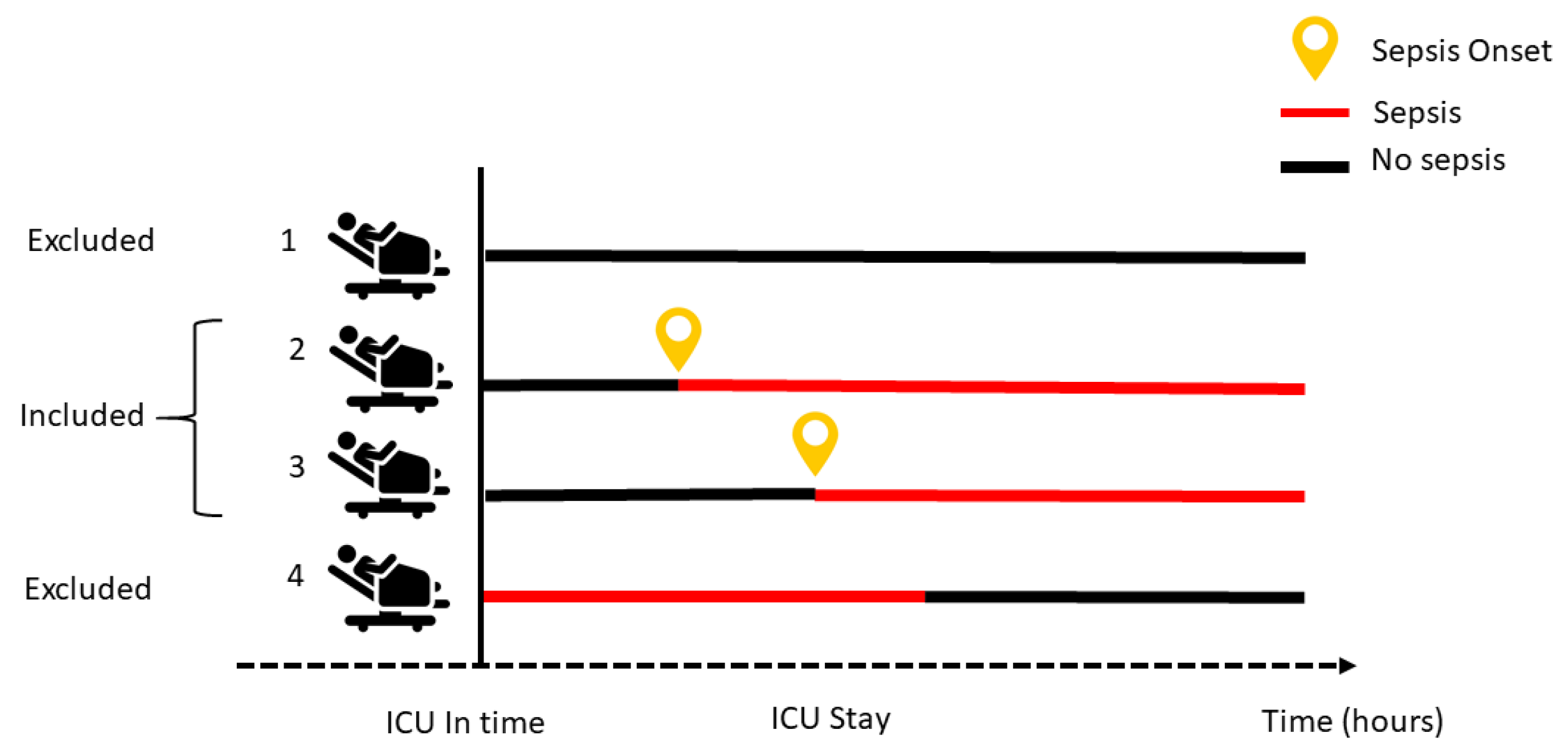
The first step of dataset preprocessing was the selection of the patient cohort. For this selection, we took into account different patient characteristics, as shown in Figure 3 and described below.

For this study, we worked only with adult patients, considering as such all patients older than 14 years. For this, following the approach proposed by [63], we used the age logged at the time of ICU admission.

For consistency and because the important data for identifying suspected infection does not appear in the CareVue system or on admission for cardio surgery, we decided to select only data collected via Meta Vision [64]. MIMIC III contains missing and outliers values during the admission and ICU stay for many reasons, including medical equipment failure, systems errors, and others. In this work, those patients with features with more than 60% missing data were entirely removed. Following the medical specialist recommendation, all the outliers were removed from the dataset. Patients that had at least three records for vital signs were selected; other features with missing data were imputed using k-nearest neighbors imputation [65].

Since the purpose of this study is the prediction of sepsis, we also excluded patients who were admitted to the ICU with sepsis, following the sepsis-3 criteria [2]. This means that we chose to focus only on those patients who developed organs dysfunctions related to sepsis at any time during the ICU stay (Figure 3).

2.3. Sepsis-3 Cohort Performance

For developing a prediction sepsis model, defining the sepsis cohort and the onset is important because this is the reference time to take the prior data. The structured approach used here yielded a well-suited cohort selection, firstly identifying the suspected infection and secondly the organs dysfunction following sepsis-3 [2,40]. To create this particular population, the sepsis-3 MIMIC III query reported by [30,59] was edited and used in Postgres. The code of the SQL query to obtain the cohort is available on Github (https://github.com/Biocamacho/Sepsis-cohort, accessed on 2 April 2022).

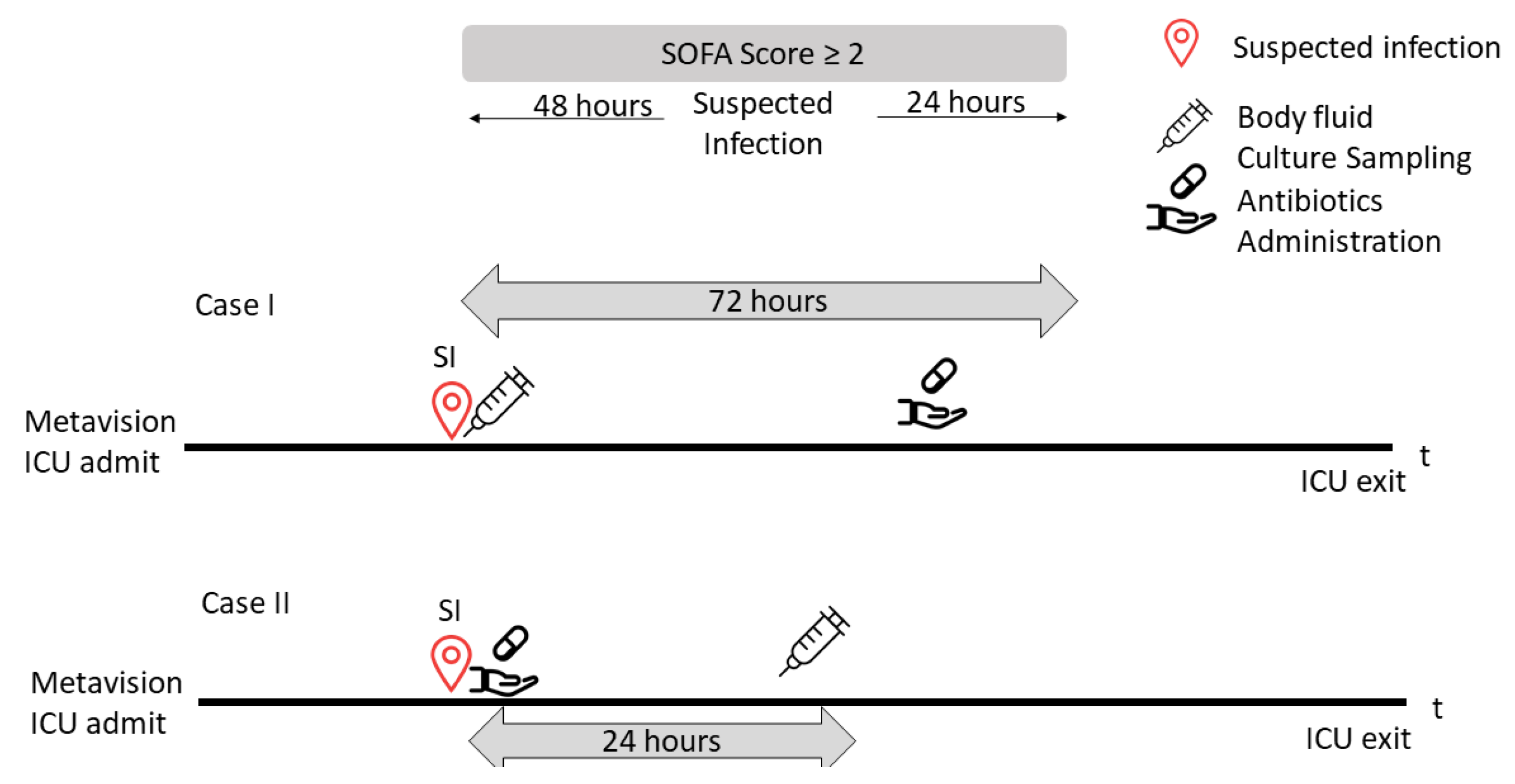
Suspected infection is defined as the administration of antibiotics and sampling of body fluid culture in a specified period. Figure 4 shows two examples, one referring to each case. Case I illustrates an example of a patient having a body fluid culture sampling at a specified time prior to antibiotics administration. In that case, the time of suspected infection was when the culture sampling was ordered. The second case (Case II) shows a patient who was administered antibiotics at a time prior to the culture sampling. In that case, the time of suspected infection was when the antibiotics were administered to the patient.

We retrieved all the timestamps of antibiotic administration and body fluid sampling over the length of ICU stay. That is, if the culture was obtained before the antibiotic, then the medication was required to be administered within 72 h, whereas if the antibiotic medication was administered first, then the sampling was required within 24 h. In this study, for each timestamp, when the first suspected infection episode was identified, we extracted the 72 h window of data for each patient, before the episode.

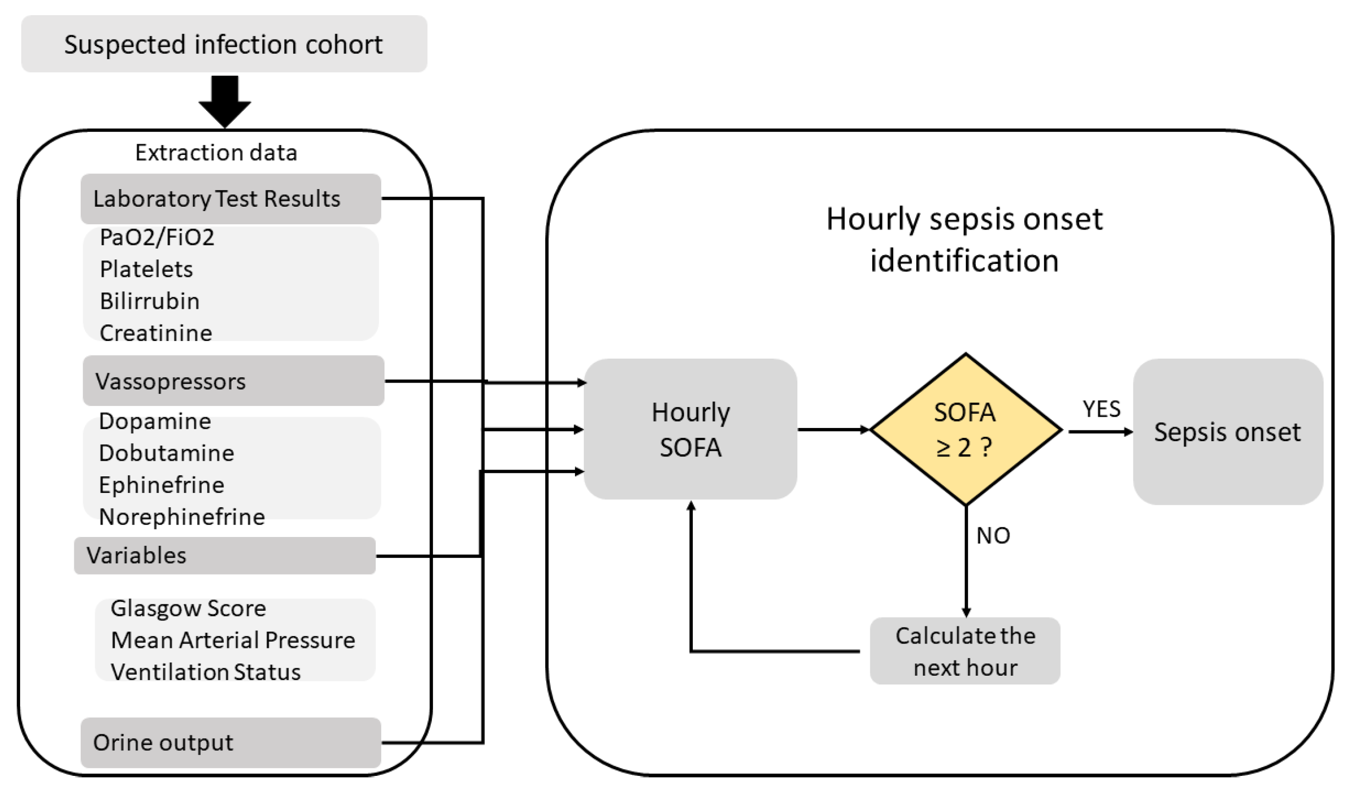
An organ dysfunction can be identified as an acute change in total SOFA ≧ 2 points consequent to the infection [23]. Afterwards, we calculated the SOFA score at each hour for the suspected infection cohort in a 72 h window, considering a period of 48 h before and up to 24 h after the onset of infection, using several queries reported by [59]. Using the Postgres function detailed in Figure 5, we extracted all the variables used in SOFA score from laboratory test results, and the Glasgow score, the ventilation status, and the vasopressors from the charted events. Finally, we labeled those patients with a SOFA score in this window increased by two or more points as “sepsis onset”.

Table 1. Summary of characteristics of the populations included in the dataset.

Variable	Sepsis	No Sepsis
n	537	1840
Diabetes (n,%)	147 (27.3%)	469 (86.2%)
Cancer (n,%)	23 (4.3%)	76 (4.1%)
Died (n,%)	39 (7.41%)	124 (6.6%)
Elixhauser comorbidity (Index)	3.01	1.52
Age (years, mean)	62.07	62.5
Weight (kg)	80.9	79.6
Days length of stay (mean)	5.9	2.17

shows the summary of characteristics of this population. The table shows how the dataset is divided in two groups: those who developed sepsis and those who did not. A total of 2377 patients met the inclusion criteria. They had a mean age of 62 years and there were no notable differences in comorbidities (diabetes, cancer, and Elixhauser index), mortality, and weight, but sepsis patients had a longer overall length of stay.

2.4. Feature Selection and Extraction

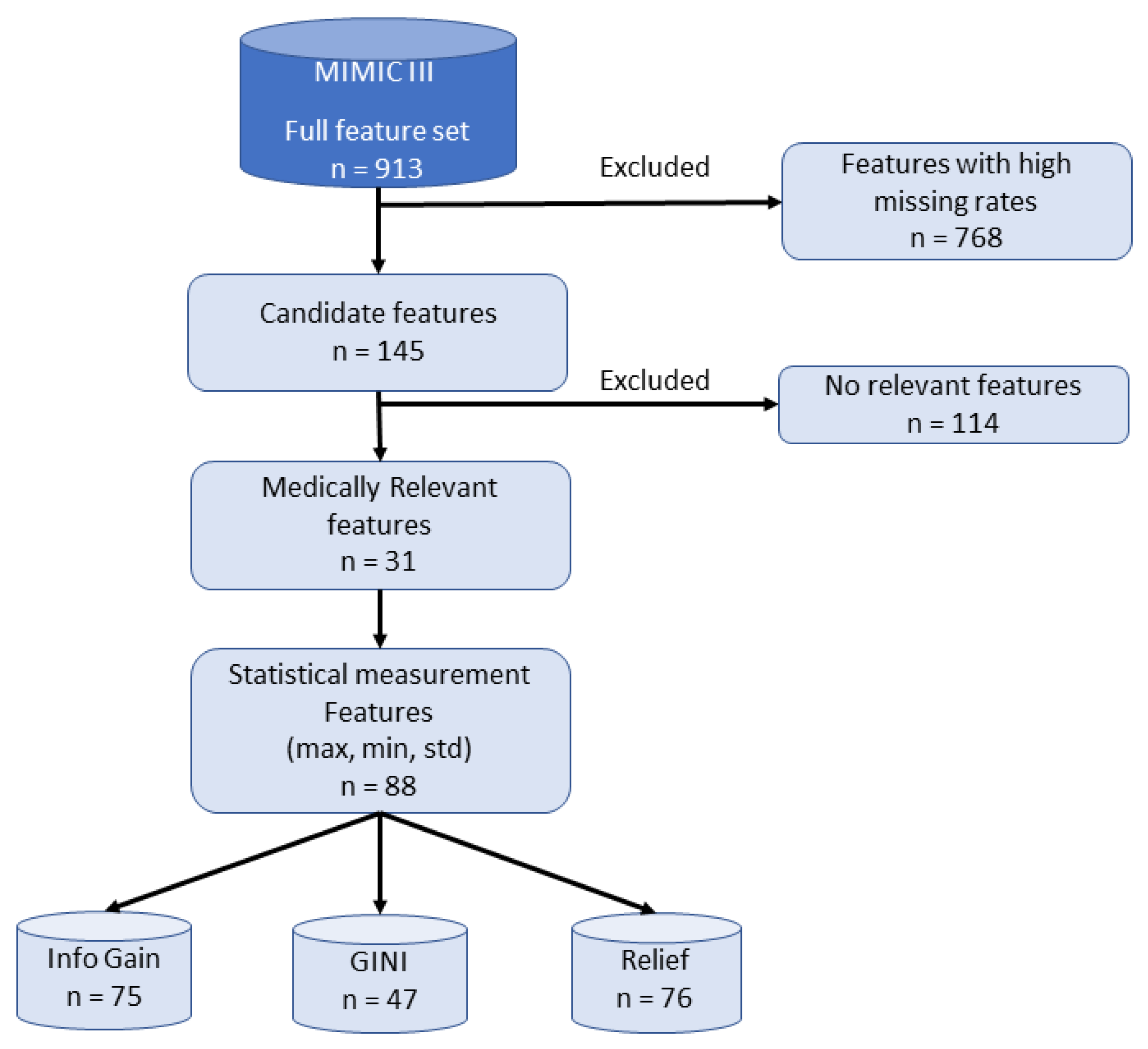
We processed the dataset to determine the candidates features to be used as input for the prediction models, excluding those features with a high missing rate, as we detail in Figure 6. In this work, the queries provided by [30,59] for the selected patient cohort were extended and refined.

In the present research, 145 features were scanned and based on the medical knowledge of an expert physician, and the 31 medically relevant features (MRF) for sepsis prediction were gathered. The complete set of patient features included was grouped into three categories: physiological data (e.g., heart rate, temperature, etc.), laboratory test results (e.g., white blood count, glucose, hematocrit, hemoglobin, creatinine, bicarbonate, PH, and arterial blood gases) and demographics/score (age, Elixhauser Index, weight, and Glasgow coma score). According to [57], we developed two engineered features to improved predictive performance: (a) shock index [66] and (b) the product of age and systolic blood pressure (min, mean, and max, labeled as FE1, FE2, and FE3, respectively). All the features included are listed in

Table 2. Final feature subset.

	Physiological features
Heart rate	Systolic blood pressure	SpO${}_2$
Diastolic blood pressure	Temperature (Celsius)	Mean blood pressure
Respiratory rate
	Laboratory test results
White blood count	Platelet	Lactate
Potassium	Glucose	Chloride
Hematocrit	Creatinine	Hemoglobin
The international normalized ratio (INR)	Prothrombin time	Bun
Thromboplastin time	Bicarbonate	Bilirubin
Ph	Creatinine	PCO2
Anion gap	Oliguria
	Demographics/Score
Age	Elixhauser Comorbidity Index	Weight
Glasgow coma score
	Feature engineered
Shock index
FE1: (Age × Min-Systolic Blood Pressure(min))	FE2: (Age × Systolic Blood Pressure(mean))	FE3: (Age × Systolic Blood Pressure(max))

. Several articles and books have mentioned those particular variables being effective and therefore should be considered during sepsis diagnosis [2,18,67].

Following [56,57,58], we calculated statistical measures including the mean, maximum (max), minimum (min), and standard deviation (std) for laboratory and physiological data. We extracted 88 statistical features from the 31 MRF to represent the patients. As shown in Figure 6, we applied a feature selection process to select the most important features prior to classification.

Feature selection has proven to be a successful preprocessing step in ML applications, building a subset of the original features with the following specific advantages: (a) avoiding overfitting, (b) improving model performance, (c) increasing speed, (d) providing cost-effective models. Feature selection methods are also classified into filters, embedded methods, and wrappers, depending on the relationship with the learning method [68]. Wrappers and embedded techniques have a higher risk of overfitting and are very computationally intensive [69]. In this study, it was preferred resorting to filter models because they are computationally simple and fast because they are independent of any learning methods, focusing on the general characteristics of the data [70]. In filter models, features are first scored and ranked according to the relevance to the class label, and then are selected based on a threshold value [71]. For each feature, each of these feature selection models has an evaluation value. Features with evaluation values greater than the threshold are chosen. Several feature selection processes exist, such as the one used by [72]. In this study, the most common filter techniques were defined to perform setting the threshold to 0.002. The filter techniques used for feature selection are: information-gain-based methods [73], relief [74], and Gini.

Table A1. Feature subset filtered using feature selection techniques.

Feature Selection Technique	Features Names
Information Gain	Glasgow (min), FE3, Systolic Blood Pressure (min), FE 2, Oliguria, Systolic Blood Pressure (mean), Respiratory Rate (min), SpO2 (max), FE 1, pCO2 (min), Mean Blood Pressure (min), glucose, glucose (min), Mean Blood Pressure (mean), Temperature (min), Bicarbonate (min), Age, Bicarbonate, Glucose (max), Temperature (mean), lactate, Elixhauser hospital, Diastolic Blood Pressure (min), Respiratory Rate (mean), ph (max), lactate (min), Heart rate (min), Lactate (std), lactate (max), SpO2 (mean), Temperature (max), Bicarbonate ((std)), Creatinine (max), Creatinine (min), Bilirubin (max), Systolic Blood Pressure (max), White Blood Count (min), Respiratory Rate (max), Creatinine, Aniongap (min), Shock Index (mean), pCO2 (max), bicarbonate (max), bilirubin (min), bilirubin, Shock Index (max), White Blood Count (max), PTT (max), INR (max), anion gap, Anion Gap (std), INR, Chloride (max), Diastolic blood pressure (mean), INR (min), PTT (min), Weight, anion gap (max), Chloride (min), PT (max), Platelet, BUN (max), Hematocrit (max), BUN (min), Platelet (min), PH (min), BUN, PT (min), Shock Index (min), Diastolic blood pressure (max), Hemoglobin (max), Platelet (max), Potassium (max)
GINI Index	FE3, oliguria, Systolic Blood Pressure (min), FE2, Systolic Blood Pressure (mean), Respiratory Rate (min), SpO2 (max), FE1, Mean Blood Pressure (min), pco2 (min), glucose, glucose (min), Mean Blood Pressure (mean), Temperature (min), Age, bicarbonate (min), glucose (max), bicarbonate, lactate, Elixhauser hospital, Temperature (mean),Diastolic blood pressure (min), lactate (min), respiratory rate (mean), lactate (std), ph (max), lactate (max), Heart rate (min), SpO2 (mean), Temperature (max), bicarbonate (std), creatinine (max), creatinine (min), White Blood Count (min), creatinine, Systolic Blood Pressure (max), Respiratory rate (max), Anion gap (min), bilirubin (max), Shock Index (mean), bicarbonate (max), White Blood Count (max), Shock Index (max), pco2 (max), PTT (max), INR (max)
Rilief	Bilirubin (min), Bilirubin, Bilirubin (max), lactate (max), lactate, pco2 (max), ph (min), ph (max), pco2 (min), lactate (min), SpO2 (min), Weight, Diastolic Blood Pressure (max), Temperature (max), INR (max), Mean Blood Pressure (max), Heart rate (max), Temperature (mean), PT (max), SpO2 (mean), Shock Index (max), Systolic Blood pressure (max), Diastolic Blood Pressure (mean), Mean blood Pressure (mean), Shock Index (mean), Respiratory rate (mean), Respiratory rate (max), INR (min), Respiratory rate (min), Mean blood Pressure (min), Temperature (min), Systolic Blood Pressure (mean), SpO2 (max), Shock Index (min), PT (min), INR, PTT (min), Platelet (std), Bicarbonate (std), Heart rate (min), FE3, Diastolic blood pressure (min), Anion gap, FE2, Heart rate (mean), Systolic blood pressure (min), White Blood count (min), FE1, Anion gap (min), Creatinine (min), White Blood Count, Potassium (max), Creatinine, Bicarbonate, Anion gap (max), Creatinine (max), White Blood Count (max), Bicarbonate (min), Bicarbonate (max), Anion gap (std), glucose (max), BUN, BUN (min), Glasgow (min), Potassium, BUN (max), Chloride (min), PTT (max), Diabetes, Glucose (min), Glucose, Chloride (max), Platelet (max)

details the features names used in every feature set.

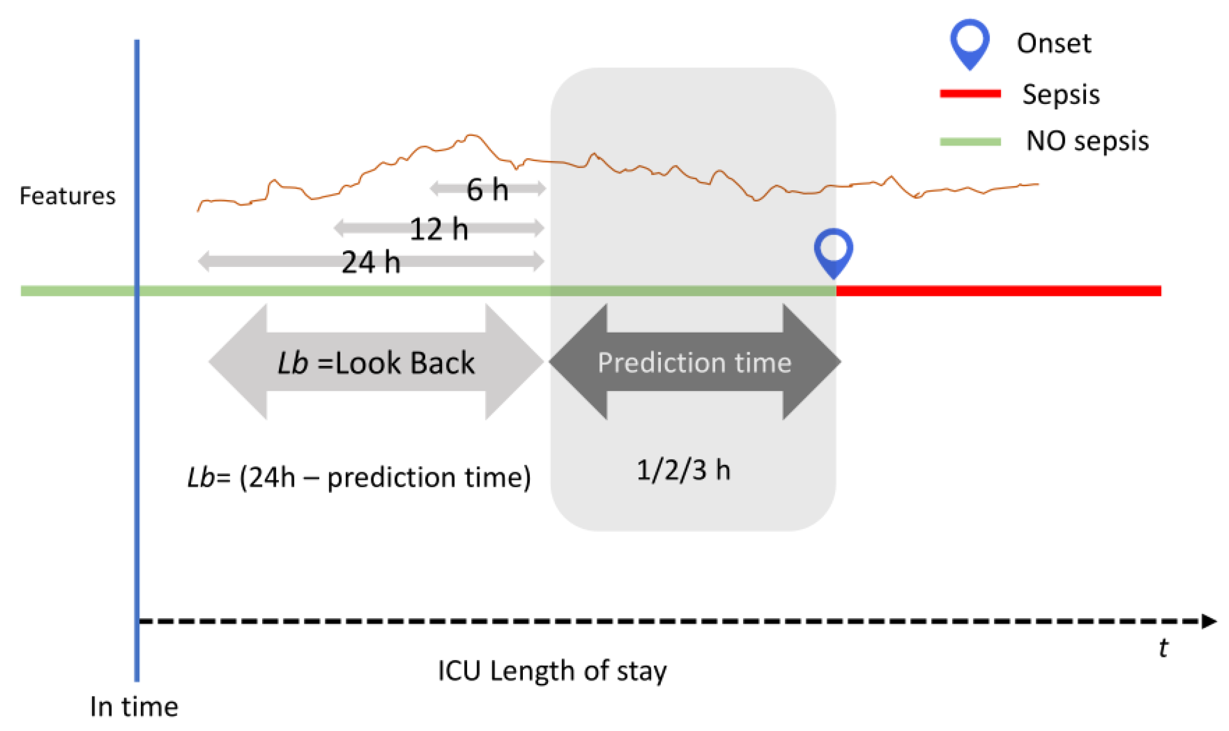
2.5. Prediction Methodology

To support the exhaustive comparison experiments, three long observational periods were considered and defined as the look back (LB) sequences of values that were used to predict. For each subset extracted earlier, three-time frames (24, 12, or 6 h) for the LB data were the inputs for the models. Finally, three horizons (1, 2, or 3 h) were defined as the prediction time to evaluate and compare the performance of all the models developed using the test set. The illustration of prediction methodology is shown in Figure 7.

2.6. Classification Models

In the present research, an experimental comparison study of traditional and ensemble supervised models of ML has been developed to predict sepsis during ICU stay. The following section defines the conventional classification models used and a few more ensemble methods.

2.6.1. Support Vector Machine (SVM)

Proposed by [75], this model is based on kernel classification to map N dimensional input data sets into a higher dimensional feature space. SVMs try to find the optimal generalization separating hyperplanes solving quadratic programming, represented by Equation (1).

$$W^t·X-b=0$$

(1)

SVMs depend on a small subset of training dataset called support vectors. In the input space, each training datum is considered as an N dimensional vector X and its label is $+1$ or $-1$.

2.6.2. K-Nearest Neighbor (KNN)

As a local classification method, KNN is based on the labels of the K-nearest patterns in data space [76]. This method assumes that all the instances correspond to points in the n-dimensional space. After defining a specific distance, a neighbor is nearest if it has the smallest distance in the n-dimensional feature space. The most commonly used distance is the Euclidean (Equation (2)).

$$d(x_i,x_j)\equiv \sqrt{\sum _{r=1}^n{\left(a_r\left(x_i\right)-a_r\left(x_j\right)\right)}^2}$$

(2)

The distance between two instances, $x_i$ and $x_j$, is defined by $d(x_i,x_j)$, where $a_r\left(x\right)$ denotes the value of the rth attribute of instance x.

2.6.3. Artificial Neural Network (ANN)

This model consists of three layers: an input layer, a hidden layer, and an output layer [76]. This layer has interconnected neurons with weights and specific activation functions. The layers transform the data and pass them to the next layer. ANN can perform the task by learning from its previous inputs. Given a network with a fixed set of units and interconnections, this network adjusts the weights using the back-propagation learning process.

2.6.4. Naïve Bayes (NVC)

This classifier applies tasks where each instance x is represented by a conjunction of attribute values and where the target function can take on any value from some finite set [76]. This model is described through the construction of a Bayesian probabilistic model that assigns a posterior class probability to an instance: [77]. The NVC uses these probabilities to assign an instance to a class, applying Bayes’ theorem, as shown in Equation (3).

$$P\left(y_j\right|x_i)=P\left(y_j\right)\frac{P\left(x_i\right|y_j)}{P\left(x_i\right)}$$

(3)

2.6.5. Random Forest (RF)

This classifier consists of a collection of classification or regression trees, which are simple models using binary splits on predictor variables to determine outcome predictions. The process is called feature sampling [78]. The trees are the base learners for RF, and the prediction is defined by classifying the data with each tree and collecting a majority rule on the whole forest. Through the bagging mechanism, each tree is built using a different bootstrap sample of the dataset.

2.6.6. AdaBoost

Adaptive boosting (AdaBoost) is defined by Freund and Schapire [79] as a boosting ensemble learning model that selects various classifier instances by preserving an adaptive weight distribution over the training examples. It is the sum of the weights of the misclassified instances divided by the total weight of all instances [80]. Following each cycle, the weight distribution is updated based on the prediction results from the training samples. The weight of correctly classified instances is reduced, while the weight of misclassified instances is increased. Thus, AdaBoost produces a set of “easy” instances that are correctly classified with low weight and a set of “hard” ones that are misclassified with high weight. In the following iteration, a classifier is built for the reweighed data, which consequently focuses on classifying the hard instances correctly. This process continues for various cycles until, finally, AdaBoost linearly combines all the component classifiers into a single final hypothesis. Greater weights are given to component classifiers with a lower training error.

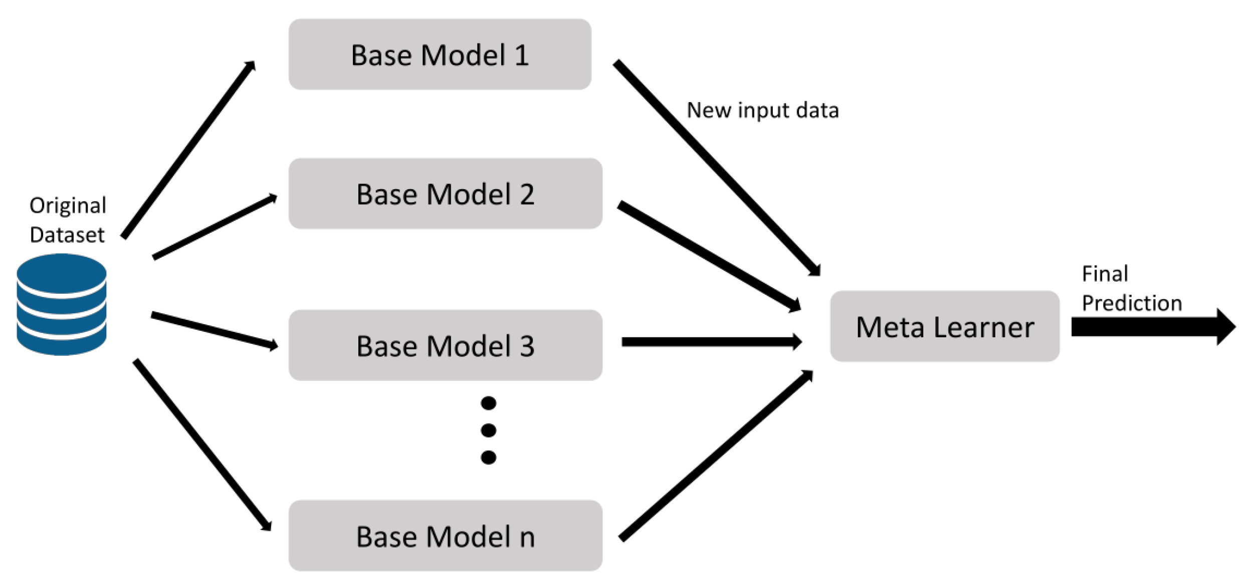
2.6.7. Stacking

Stacking is an ensemble learning technique that combines in parallel a set of different classifiers by training a meta-classifier to output a strong prediction based on the various models predictions [81]. Figure 8 shows the stacking model, which implements the following steps: first, all the base models compute on the original dataset; second, the predictions made by these classifiers are considered as a new input data to the final model; eventually, a learning process occurs using this new input to obtain a final prediction.

2.6.8. XGBoost

Extreme gradient boosting (XGBoost) [82] is another ensemble of classifiers, considered as an optimized gradient tree boosting model, based on algorithmic optimizations and hyperparameters to perform the learning process and control the overfitting. The most important factor behind the XGBoost model is the tree learning algorithm for handling sparse data. XGboost use an objective function to optimize the loss function, considering the results from the previous level, and adds regularization to perform the results.

2.7. Performance Metrics and Model Evaluation Procedures

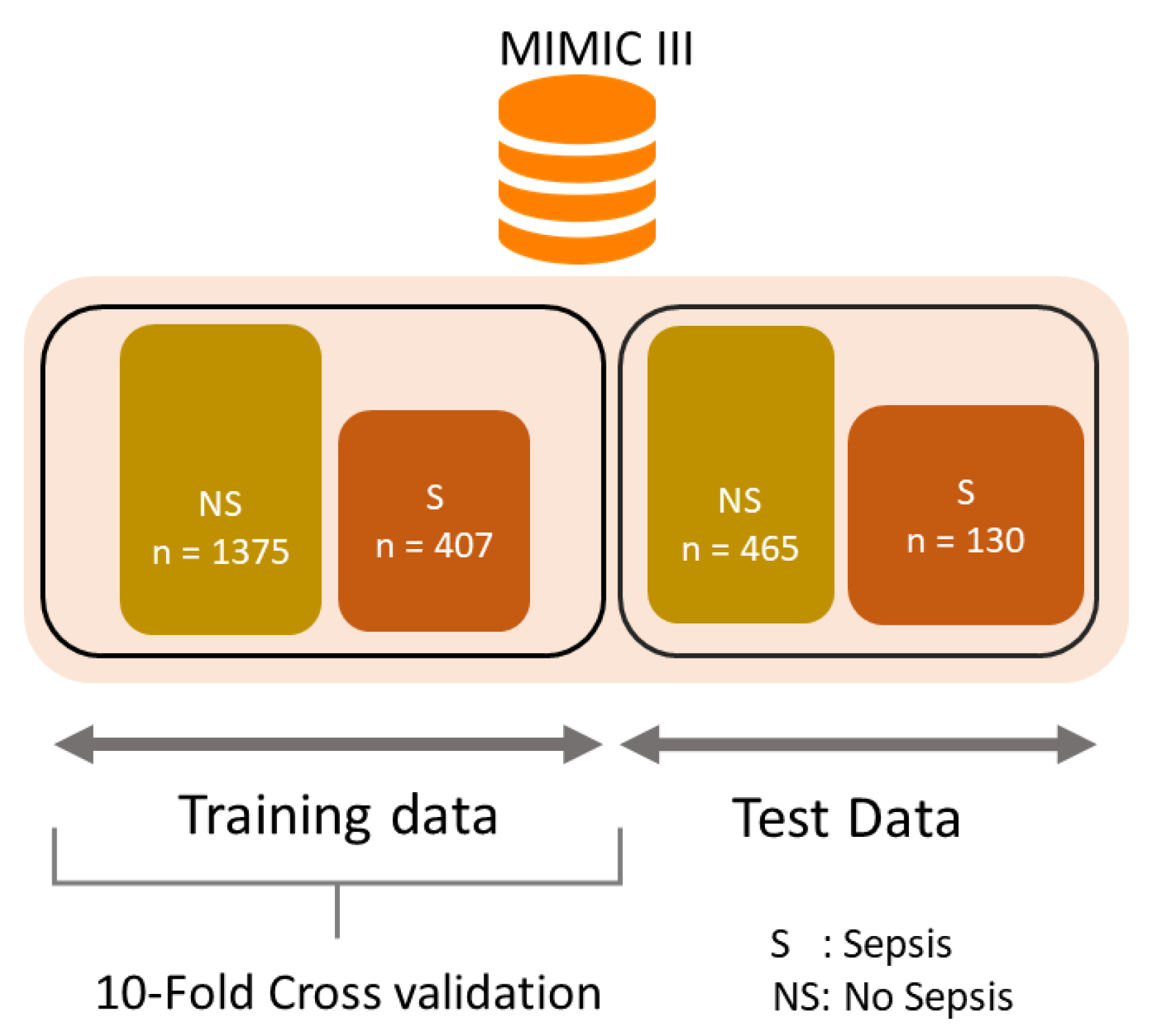
To evaluate all the predictions models train–test split procedure and k-fold cross-validation were used as model evaluation procedures. The dataset was randomly divided into training set (75%) and test set (25%).

Figure 9 shows the structure of train and test data sets. In this study, a 10-fold cross-validation method was used for selecting the best model for training [76]. Cross-validation is defined as a method for the evaluation of the performance of a predictive model. Statistical analysis will generalize to an independent dataset. K-fold cross-validation is a method for dividing the original sample randomly into K sub-samples. The model is then tested using a single sub-sample as validation data, while the remaining $K-1$ sub-samples are used as training data. These process is repeated K times, with one of the K sub-samples representing as the validation data.

Class imbalance is a particular problem in medical datasets. In MIMIC-III, a majority patient had no sepsis (94.5%) and a minority of patients were sepsis diagnosed (5.5%) during ICU Stay. Two techniques are the most commonly used for data sampling: oversampling and undersampling. The latter, according to the research, has shown to be the superior option over oversampling [83,84]. In this research, the random undersampling technique was used to improve the data balance by removing patients from the prevalent class (no sepsis). Therefore, the undersampling process cut the sample to 2377 patients (77.4% no sepsis; 22.5% sepsis).

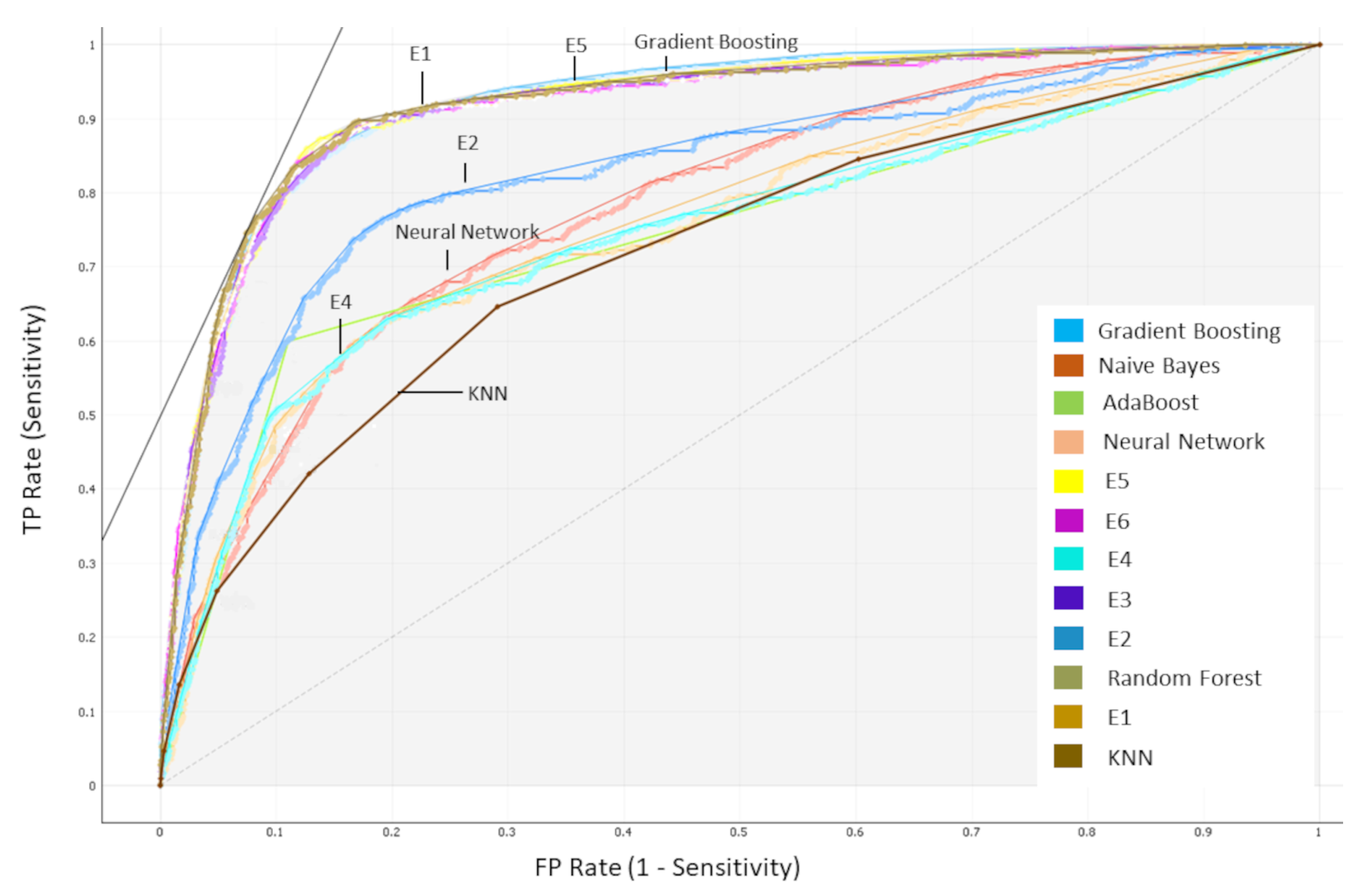
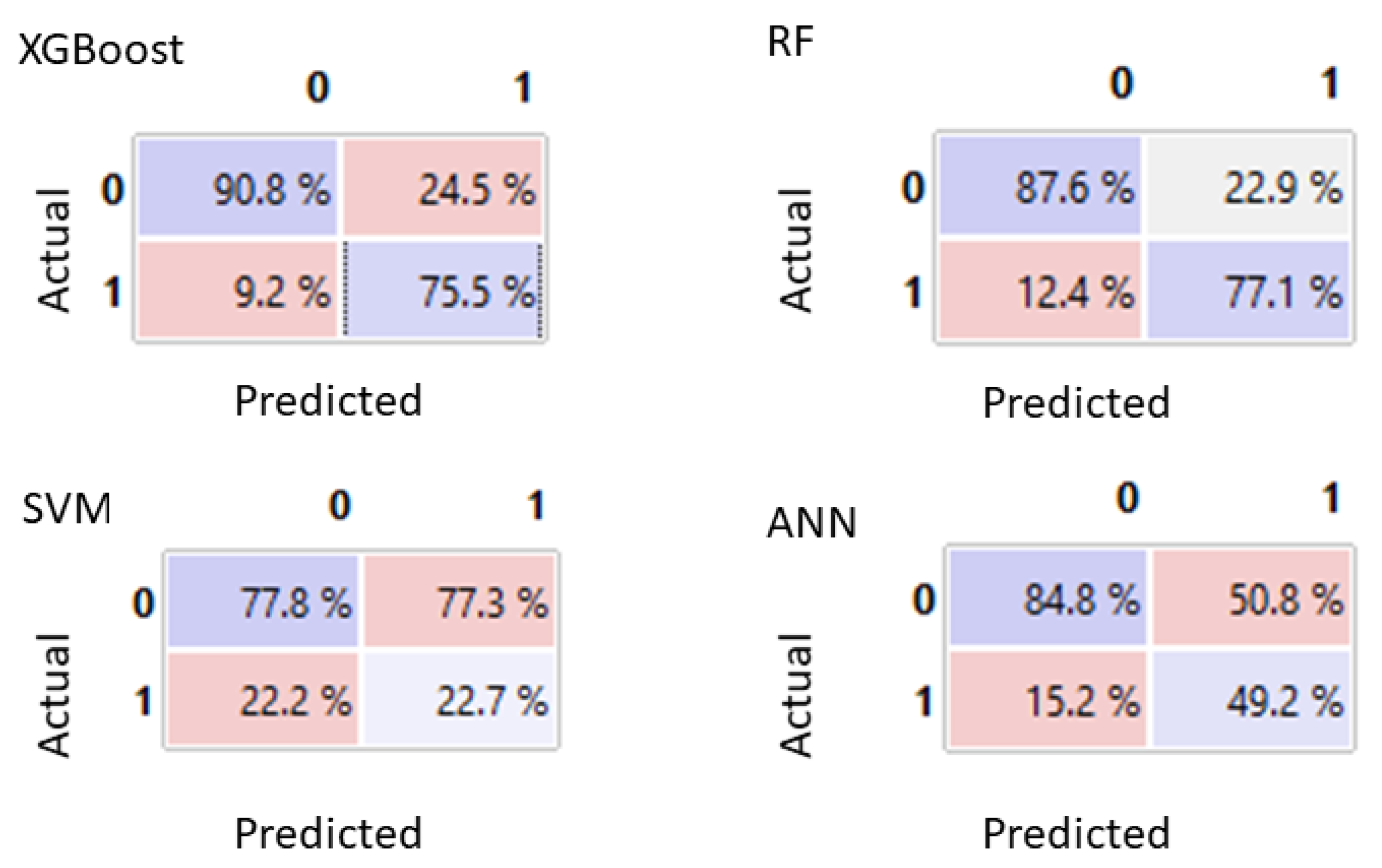
For each model included in this study, different metrics were obtained to evaluate the performance according to [85]: area under receiver operating characteristic (AUC-ROC), accuracy, F1 score, recall, specificity, and precision as the evaluation metrics to report results. A binary classification allows to create a confusion matrix, as shown in

Table 3. Confusion matrix.

		Predicted
		Positive	Negative
True	Positive	TP	FN
	Negative	FP	TN

, based on the following four categorizations of predictions:

• True positives (TP): instances correctly labeled as positive.
• False positives (FP): negative instances incorrectly labeled as positive.
• True negatives (TN): instances correctly labeled as negative.
• False negatives (FN): positive instances incorrectly labeled as negative.

Accuracy measures indicate that the overall proportion of labels were correctly identified.

$$Accuracy=\frac{TP+TF}{TP+TF+FP+FN}$$

(4)

$F1$ score is defined as the harmonic mean of $Recall$ and $Precision$ that sets their trade-off.

$$F1=\frac{2\ast Precision\ast Recall}{Precision+Recall}=\frac{2TP}{2TP+FP+FN}$$

(5)

$Recall$ indicates the proportion of correctly predicted sepsis cases from the sepsis set.

$$Recall=\frac{TP}{TP+FN}$$

(6)

Likewise, specificity represents the proportion of correctly predicted no-sepsis cases among the no-sepsis group. The AUC-ROC value considers the sensitivity against the specificity at various threshold settings. Lastly, $Precision$ gives us the proportion of cases which were identified as having sepsis who actually had sepsis.

$$Precision=\frac{TP}{TP+FP}$$

(7)

The performance of each classifier was evaluated with a number of comparisons including qSOFA and SOFA Score.

2.8. Selection of Classification Models

Several comparison experiments were performed using the following conventional classification models: SVM, KNN, RF, ANN, Naïve Bayes, and the combination with ensemble models: boosting (Adaboost and XGBoost) and stacking schemes.

An ensemble selection approach was used to achieve improved performance. The models were implemented in Orange version 3.31 [86] and Phyton using Google Colab infrastructure [87].

In the present study, three different prediction times (pt = 1/2/3 h) were considered. Therefore, nine different data collections were produced considering the different LB defined. For all the developed models, the performances were evaluated and compared against the traditional medical scores: the qSOFA and the SOFA Score.

3. Results and Discussion

In the present study, extensive experiments were performed to compare the results of conventional classification and ensemble models using the MIMIC III dataset including vital signs, laboratory test results, and demographics. To obtain a cohort, a balance strategy was conducted, which includes the 2377 patients (537 cases and 1840 controls) from undersampling process. In this study, the objective was to develop a model for early sepsis prediction in the ICU. This work presented an experimental investigation of the combination of heterogeneous learning algorithms to develop a more accurate ensemble model. Following an ensemble selection approach, a total of six ensemble models were finally selected to achieve improved performance. Other ensemble models were tested, but did not produce accurate results compared to the six previous models. As can be seen in

Table 4. Description of ensemble models developed.

Ensemble	Label	Models
	E1	RF + SVM
	E2	ANN + AdaBoost
	E3	RF + ANN
	E4	SVM + ANN
Stack	E5	SVM + ADA + ANN + KNN + RF + Tree
	E6	ANN + KNN + RF + SVM + Tree

, E1 to E6 consist of stacking ensemble models with logistic regression as the aggregation algorithm. To obtain the most optimized results for all the models developed the hyperparameters were tuned,

Table 5. Model hyperparameter used.

Algorithm	Hyperparameter
KNN	Neighbors = 7, Metric = Euclidean, Weight = Uniform
Random Forest	Number of Trees = 300, Number of attributes considered at each split = 10
Neural Network	Layers = 4, Number of neurons in hidden Layers = (40, 20, 10, 5), Solver = Adams, Activation = tah, Maximal number of iteration = 1000
Adaboost	Base estimator = Tree, Number of estimator = 100, Learning rate = 1.0, Fixed seed for random generator = 5, Classification algorithm = SAMME.R, Regression loss function = Linear
Tree	Min number of instances in leaves = 4, Max tree depth = 100
Support Vector Machine	Cost = 1.60, Regression loss epsilon = 0.40, Kernel = linear, numerical tolerance = 0.0010

shows details. As a result, the stacking model is expected to outperform all models.

Results of Feature Selection

In the present study, the performance of five conventional classifiers were evaluated—KNN, random forest, ANN, Naïve Bayes, SVM, and ensemble models—by tuning the hyperparameters and testing the following three feature selection techniques to obtain the most optimized results: information gain, GINI index, and relief. The feature selection allows the reduction in dimension of data and improves the performance of classification and ensemble models using the best subset of features. Features were selected according to their importance using the 10-fold cross validation. For example, it is important to consider the minimum value for Glasgow score. For laboratory test results, the minimum and maximum values were considered. For example, high hemoglobin can be a sign of blood thickness, which may lead to strokes. Low values of hemoglobin may also be a risk indication of kidney disease. Table A1 shows the relevant feature subset filtered using feature selection techniques.

In this experiment, the role of feature selection techniques was explored to enhance the performance of the ML algorithms. The results have been reported in

Table 6. Comparison of models results based on feature selection techniques using t = 1 h and look back 24 h.

Model	Feature Selection Technique	AUC-ROC	Accuracy	Recall	Precision
E1		0.902	0.870	0.769	0.779
E2		0.824	0.725	0.675	0.0.613
E3		0.903	0.735	0.635	0.642
E4		0.811	0.605	0.570	0.585
E5		0.895	0.863	0.839	0.839
E6		0.893	0.873	0.813	0.819
XGBoost	Information Gain > 0.002	0.918	0.872	0.852	0.868
Random Forest		0.905	0.866	0.852	0.860
ANN		0.753	0.804	0.734	0.795
Naïve Bayes		0.780	0.792	0.719	0.779
KNN		0.721	0.796	0.719	0.769
SVM		0.231	0.459	0.419	0.664
E1		0.754	0.810	0.714	0.797
E2		0.724	0.589	0.573	0.561
E3		0.757	0.809	0.788	0.782
E4		0.738	0.587	0.563	0.573
E5		0.759	0.807	0.703	0.739
E6		0.758	0.809	0.740	0.644
XGBoost	GINI > 0.002	0.755	0.795	0.787	0.770
Random Forest		0.752	0.812	0.802	0.807
ANN		0.643	0.743	0.734	0.726
Naïve Bayes		0.726	0.769	0.719	0.758
KNN		0.669	0.785	0.719	0.750
SVM		0.517	0.431	0.419	0.668
E1		0.904	0.874	0.852	0.870
E2		0.813	0.822	0.813	0.790
E3		0.906	0.865	0.813	0.803
E4		0.802	0.813	0.801	0.8141
E5		0.890	0.868	0.812	0.824
E6		0.909	0.837	0.814	0.812
XGBoost	Reflief > 0.002	0.909	0.856	0.849	0.832
Random Forest		0.752	0.812	0.802	0.807
ANN		0.782	0.790	0.734	0.791
Naïve Bayes		0.799	0.790	0.69	0.763
KNN		0.744	0.794	0.774	0.766
SVM		0.543	0.425	0.419	0.677

, presenting AUC-ROC, accuracy, recall, and precision, using pt = 1 h, lb = 24 h, and 10-fold cross validation.

The results exhibit high recall and AUC-ROC when predicting sepsis through ensemble models and implementing information gain feature selection. Interestingly, information gain demonstrated better results for conventional and ensemble classification models, compared with the others feature selection techniques using 24 h dataset. For information gain feature selection we observed that XGBoost and random forest generate the best testing results. The XGBoost algorithm achieves values of AUC-ROC = 0.918, accuracy = 0.872, recall = 0.852, and precision = 0.868. The random forest reported an AUC-ROC = 0.905, accuracy = 0.866, recall = 0.852, and precision = 0.860. Conversely, ANN, SVM, and KNN models shows the worst results. The confusion matrix is used to identify proportions of instances between the predicted and actual class. The number of false positives and false negatives can also be seen in this matrix. Figure 10 shows the confusion matrices of XGBoost, RF, SVM, and ANN models, respectively.

For the GINI feature set, the overall testing results were worsened by 6–16 % in terms of AUC-ROC, accuracy, recall, and precision. The random forest, E1, and E5 models achieved the best testing results. In particular, E1 test results are AUC-ROC = 0.759, accuracy = 0.810, recall = 0.714, and precision = 0.797. Random forest showed the following performance: AUC-ROC = 0.752, accuracy = 0.812, recall = 0.802, and precision = 0.807. For feature set filtered by relief, the overall testing performance was improved compared to GINI sets. XGBoost and E1 offer the best performance with AUC-ROC = 0.909–0.904, accuracy = 0.876–0.874, recall = 0.869–0.852, and precision = 0.872–0.870, respectively. Figure 11 compares the AUC-ROC curves for these ML algorithms based on information gain sets.

Feature selection techniques improve the results and stability of the ML algorithms and reduce the noise. From these previous experiments, we observed that the feature set selected using information gain achieved the best results.

The test set was used to validate the ML models and to explore their generalization capabilities. For this, the three sliding windows of 6, 12, and 24 h were used.

A statistical comparison is applied to evaluate the performance of all candidates models using 1, 2, and 3 h of prediction time for the three LB windows, as shown in

Table 7. Detailed results of model evaluation using 24 h of look back data and 1, 2, and 3 h prediction time.

Look Back = 24 h
		t = 1			t = 2			t = 3
Model	Accuracy	Recall	AUC-ROC	Accuracy	Recall	AUC-ROC	Accuracy	Recall	AUC-ROC
E1	0.859	0.645	0.773	0.853	0.618	0.778	0.851	0.618	0.765
E2	0.811	0.605	0.735	0.811	0.605	0.734	0.811	0.605	0.735
E3	0.803	0.567	0.773	0.813	0.521	0.707	0.814	0.519	0.708
E4	0.811	0.605	0.693	0.795	0.511	0.692	0.795	0.514	0.694
E5	0.861	0.563	0.907	0.859	0.559	0.906	0.862	0.563	0.907
E6	0.862	0.570	0.909	0.862	0.561	0.910	0.864	0.574	0.910
XGBoost	0.864	0.687	0.919	0.856	0.668	0.916	0.847	0.646	0.911
SVM	0.411	0.712	0.506	0.411	0.712	0.506	0.411	0.712	0.506
AdaBoost	0.811	0.600	0.735	0.811	0.600	0.735	0.811	0.600	0.735
RF	0.908	0.532	0.908	0.858	0.538	0.908	0.862	0.540	0.909
ANN	0.795	0.506	0.817	0.795	0.506	0.817	0.795	0.506	0.817
KNN	0.780	0.445	0.768	0.780	0.445	0.768	0.870	0.445	0.768

,

Table 8. Detailed results of model evaluation using 12 h of look back data and 1, 2, and 3 h prediction time.

		t = 1			t = 2			t = 3
Model	Accuracy	Recall	AUC-ROC	Accuracy	Recall	AUC-ROC	Accuracy	Recall	AUC-ROC
E1	0.848	0.671	0.660	0.831	0.567	0.621	0.821	0.525	0.618
E2	0.809	0.579	0.725	0.801	0.548	0.709	0.794	0.532	0.674
E3	0.796	0.525	0.696	0.793	0.491	0.683	0.797	0.504	0.672
E4	0.786	0.480	0.674	0.786	0.474	0.674	0.788	0.487	0.668
E5	0.853	0.532	0.889	0.837	0.490	0.888	0.829	0.440	0.880
E6	0.856	0.533	0.902	0.886	0.488	0.886	0.829	0.540	0.880
XGBoost	0.850	0.665	0.912	0.851	0.643	0.907	0.838	0.614	0.896
SVM	0.347	0.714	0.467	0.399	0.760	0.519	0.382	0.760	0.521
AdaBoost	0.809	0.557	0.725	0.801	0.547	0.709	0.793	0.531	0.699
RF	0.855	0.527	0.902	0.842	0.495	0.887	0.831	0.448	0.883
ANN	0.779	0.513	0.785	0.784	0.483	0.806	0.784	0.513	0.811
KNN	0.786	0.391	0.762	0.788	0.373	0.776	0.773	0.403	0.769

and

Table 9. Detailed results of model evaluation using 6 h of look back data and 1, 2, and 3 h prediction time.

		t = 1			t = 2			t = 3
Model	Accuracy	Recall	AUC-ROC	Accuracy	Recall	AUC-ROC	Accuracy	Recall	AUC-ROC
E1	0.848	0.648	0.772	0.820	0.527	0.738	0.811	0.499	0.729
E2	0.796	0.573	0.716	0.789	0.537	0.699	0.789	0.537	0.695
E3	0.800	0.485	0.648	0.799	0.504	0.695	0.791	0.443	0.663
E4	0.784	0.472	0.669	0.784	0.514	0.687	0.777	0.419	0.646
E5	0.853	0.494	0.883	0.829	0.439	0.880	0.857	0.373	0.857
E6	0.857	0.552	0.887	0.886	0.488	0.886	0.818	0.352	0.856
XGBoost	0.861	0.659	0.900	0.845	0.621	0.893	0.840	0.604	0.886
SVM	0.367	0.792	0.526	0.382	0.760	0.513	0.356	0.783	0.488
AdaBoost	0.794	0.453	0.776	0.793	0.531	0.699	0.788	0.531	0.695
RF	0.855	0.526	0.888	0.827	0.436	0.882	0.822	0.450	0.865
ANN	0.793	0.482	0.789	0.784	0.513	0.811	0.774	0.440	0.787
KNN	0.797	0.370	0.779	0.773	0.403	0.769	0.772	0.357	0.764

, respectively. The results confirm the effectiveness in achieving higher accuracy of ensemble learning techniques in comparison with single classifiers. In particular, the stacking ensemble method was applied to achieve a more accurate sepsis prediction for time prediction = 1 h and look back = 24 h (E5 AUC-ROC = 0.907, E6 AUC-ROC = 0.910) compared with other ensemble models (E1, E2, E3, and E4). One interesting observation is that SVM reveals a high recall and the poorest for the other metrics. Likewise, RF exhibits high performance in accuracy and AUC-ROC. Detailed numerical results in Table 7, Table 8 and Table 9, show the XGBoost model provides better results for various prediction windows and look back dataset. The XGBoost model obtains permanent best results, even for t = 3 achieving AUC-ROC = 0.911, 0.896, and 0.886 for various LBs. The performance decreased in all models when increasing the prediction time.

Information gain contains 75 features and we found that Glasgow, weight, temperature (min), and hematocrit (max) were the five most important ones for prediction sepsis using XGBoost algorithm, as shown in Figure 12. For interpreting the effects and relative contributions of selected features and clinical parameters on sepsis prediction, an explainer Shapley additive explanation (SHAP) SHAP was implemented [88]. A tree SHAP algorithm was used to explain the output of XGBoost models. Tree SHAP is a fast and exact method to estimate SHAP values for tree models and ensembles of trees [89]. The bee swarm plot, Figure 13, shows how the value of each feature impacts model output. The color on the right side represents the feature value; red represents a higher value; and blue represents a lower value. As expected, the Glasgow scale, temperature, glucose, $Sp{O}_2$, and heart rate were identified as the most significant contributors. In addition, the blood pressure and laboratory test results (PH and bilirubin) also contribute to the sepsis prediction.

The findings confirm the factor behind the success of the XGBoost model revealed [82], for instance the tree learning technique for handling sparse data and the scalability through algorithmic optimizations.

The ensemble models E1, E5, E6 and XGBoost exhibit higher results compared to others models in all computed scenarios. They were selected for comparison with two standard severity scores—SOFA and qSOFA. Figure 14 shows the results using one hour for time prediction and 24 h for the LB features. The selected ensemble showed higher performance in terms of accuracy, recall, F1, and AUC-ROC. This may explain the strong results during the ensemble model E1. In particular, the XGBoost model formed better than all other models, achieving a superior performance.

4. Conclusions

Early diagnosis and an appropriate antibiotic therapy of sepsis is crucial but sometimes challenging. Several patient-health-score-based prediction systems have been employed for evaluating the early detection of patient deterioration. However, these scoring systems are useful for predicting general deterioration or mortality, but cannot identify sepsis in patients with high sensitivity and specificity at individual level. The increasing availability and the versatility of healthcare data suggest to implement ML techniques to develop models for predicting sepsis.

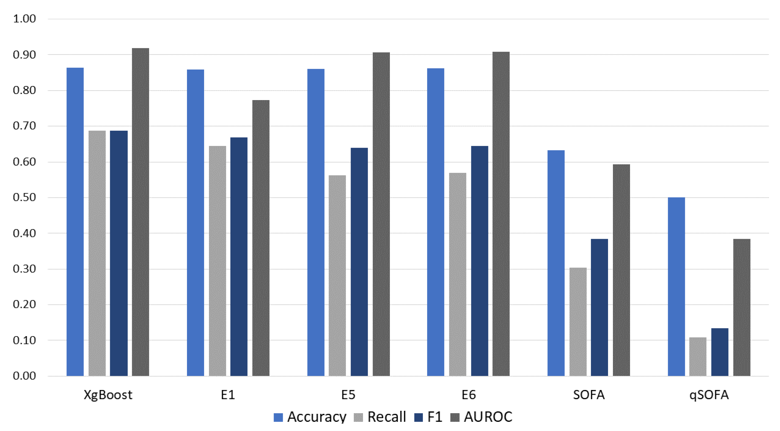
In this study, several ML-based models were applied for sepsis prediction using vital signs, laboratory test results, and demographics variability. The results demonstrate overall higher performance of ML models over the commonly used SOFA and qSOFA scoring systems at the time of sepsis onset.

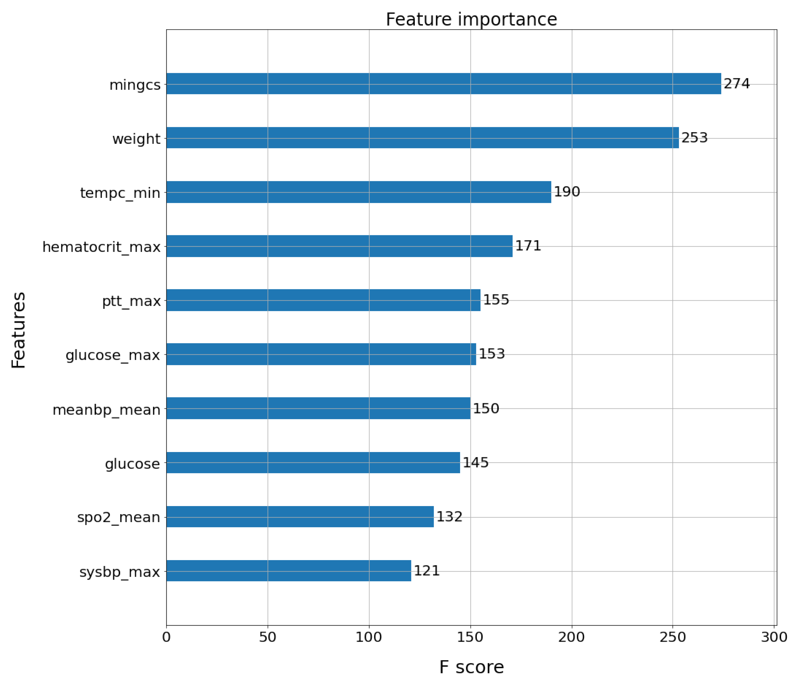
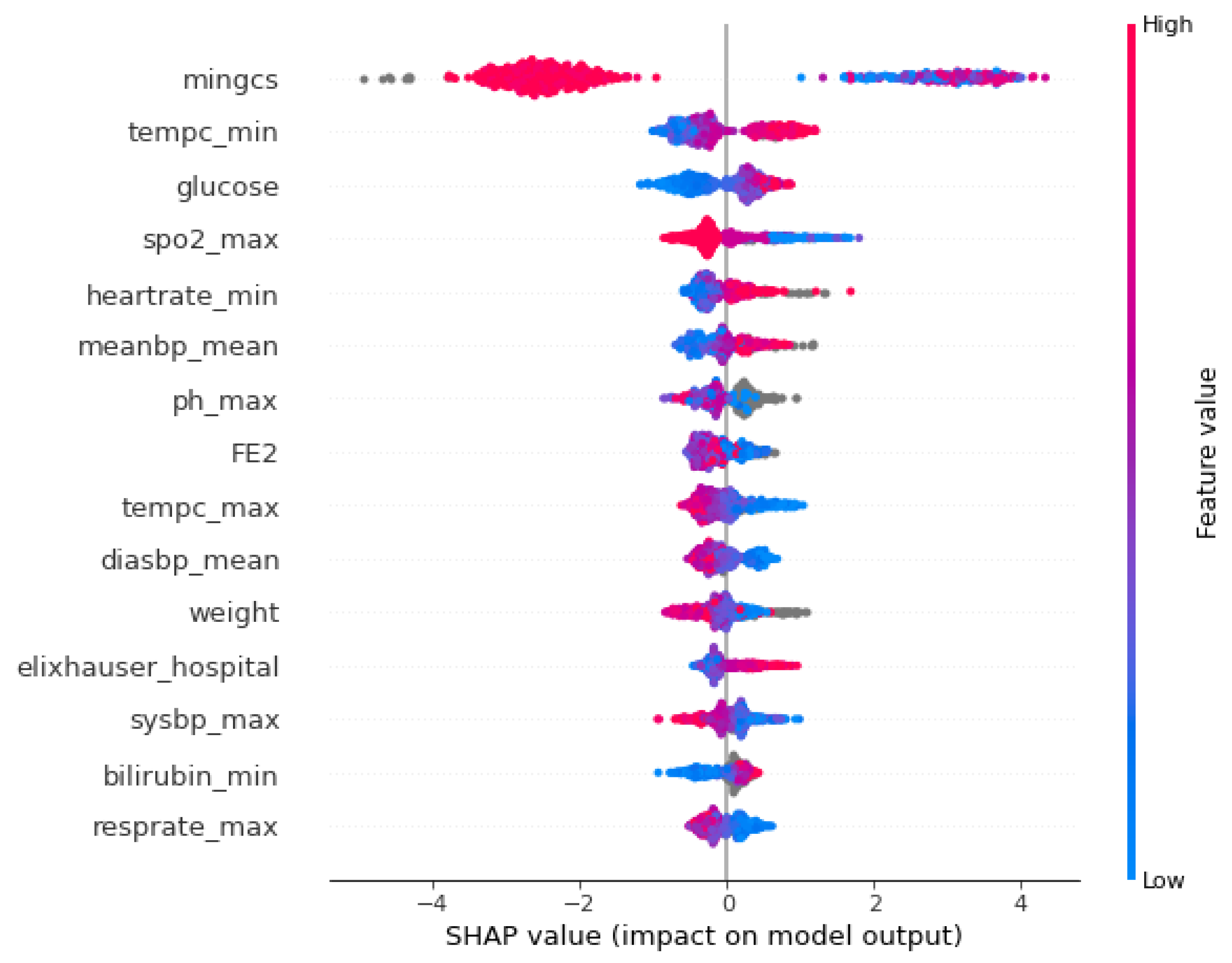
The results reveal high metrics when using ensemble models and feature selection strategies for predicting sepsis. Particularly, this study demonstrated better results for information gain compared with conventional feature selection techniques. The addition of some variables from laboratory test results as input variables overall increases the model performance.

This work provides a consistent set of comparison of ML models for sepsis early prediction on the large healthcare datasets, following the sepsis-3 definition and selecting features in a meaningful way. The results are a strong motivator for implementing these ensemble models for early sepsis prediction in ICU cases.

In this study, the 12 ML models were computed with various feature windows for 1, 2, and 3 h of sepsis prediction. The ensemble models combining the variability of physiological data and laboratory test results, as well as demographics values, outperformed all the conventional algorithms. They also showed a large margin of improvement over traditional scoring systems at the time of sepsis onset. The best results were obtained using the XGBoost model implementing the information gain feature selection technique, achieving 0.911 AUC-ROC for 24 h of look back data in a t = 1 h prediction time.