
A Novel Anti-Risk Method for Portfolio Trading Using Deep Reinforcement Learning

Abstract
:1. Introduction
2. Preliminary
2.1. Problem Setup
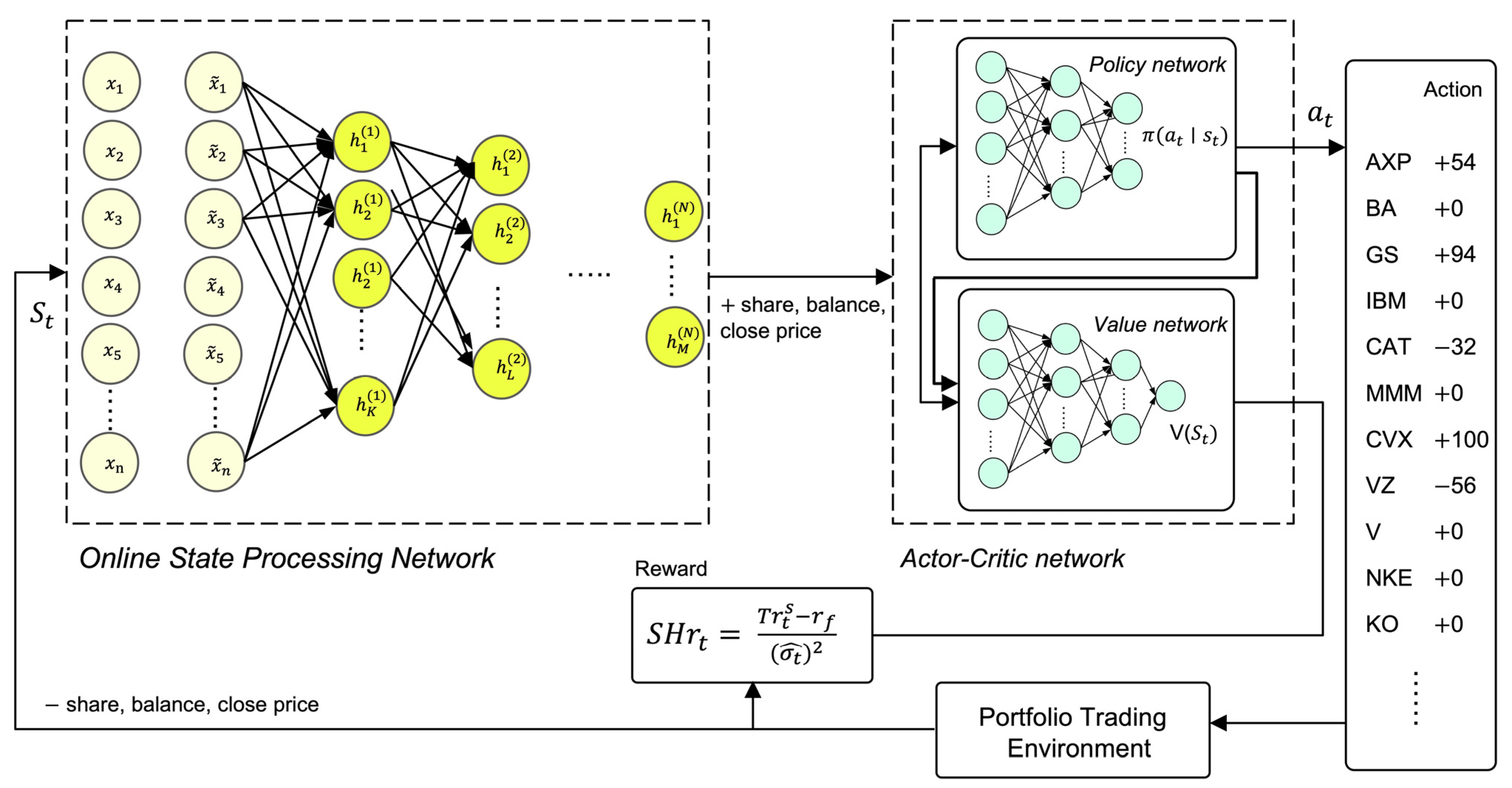
2.1.1. State Space
- ∈ :available balance at current time step t.
- ∈ : shares owned of each stock at current time step t.
- ∈ : close price of each stock at current time step t.
- ∈ : encoding features at current time step t.
2.1.2. Action Space
2.1.3. Reward Function
2.2. Trading mode
- The trading volume of the agent is very small compared to the size of the whole market, so the agent’s trades do not affect the state transition of the market environment.
- The liquidity of the market is high enough that the orders can be rapidly executed at the close price.
- The transaction cost is a fixed proportion of the trade volume of the day.
3. Methodology
3.1. Depiction of Stock Markets
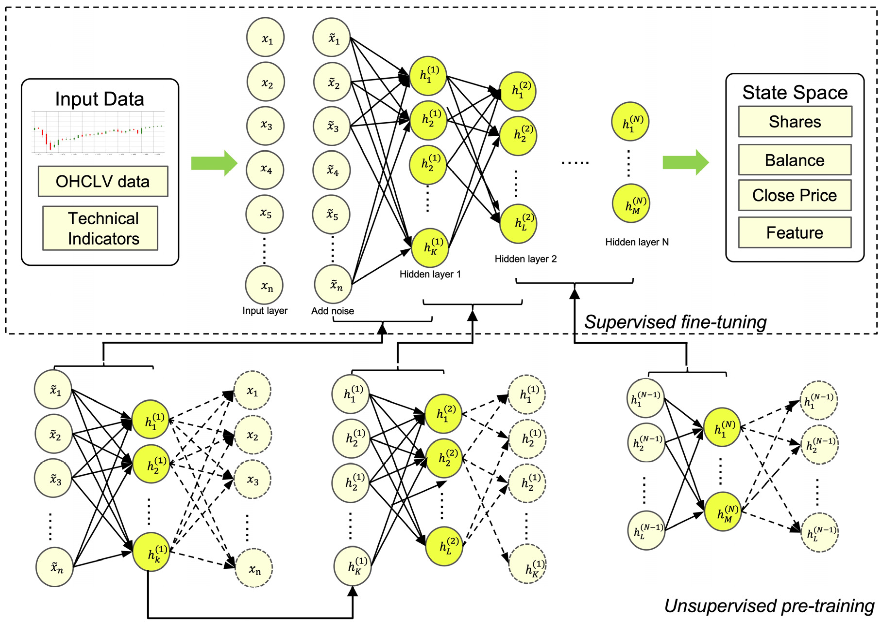
3.2. Overview of SSDAE
3.2.1. Sparse Denoising Autoencoder (SDAE)
3.2.2. Stacked Sparse Denoising Autoencoders (SSDAE)
3.3. Optimization via Reinforcement Learning—Advantage Actor–Critic Learning
4. Experiments
4.1. Dataset Descriptions
4.2. Evaluation Metrics
- Cumulative return (CR): is the total amount earned by an RL agent during the trading period, excluding transaction costs.
- Maximum drawdown (MDD) [25]: refers to the maximum loss percentage from peak to trough during the trading period.
- Sharp ratio (SR): Sharp ratio [26] is used to measure the rate of return that trading strategies can achieve when confronted with a unit of risk. It is the most commonly used mainstream standardized metric for evaluating portfolio strategies’ performance. Equation (5) has illustrated the calculating formula.
- Calmar ratio (CMR): Calmar ratio [27] is used to measure the risk by using the concept of MDD.
- Alpha: Alpha value is used to measure the excess return obtained by the model relative to the benchmark within the trading range. The greater the alpha value, the more capable it is of generating additional returns in comparison to the benchmark. The calculation process of alpha value is shown in:where is the yield of the model, is the beta value of the model, and is the yield of the benchmark strategy.
- Beta: Beta value is an indicator used to assess the systemic risk of the model relative to the benchmark. If the beta value is greater than one, the volatility of the model is greater than the benchmark; if the beta value is less than one, the volatility of the model is less than the benchmark; and if the beta value is equal to one, the volatility of the model is the same as that of the benchmark. The computation method is illustrated below:where is the covariance, and is the variance of the benchmark strategy.
4.3. Experimental Details
4.4. Discussion of Comparison Methods
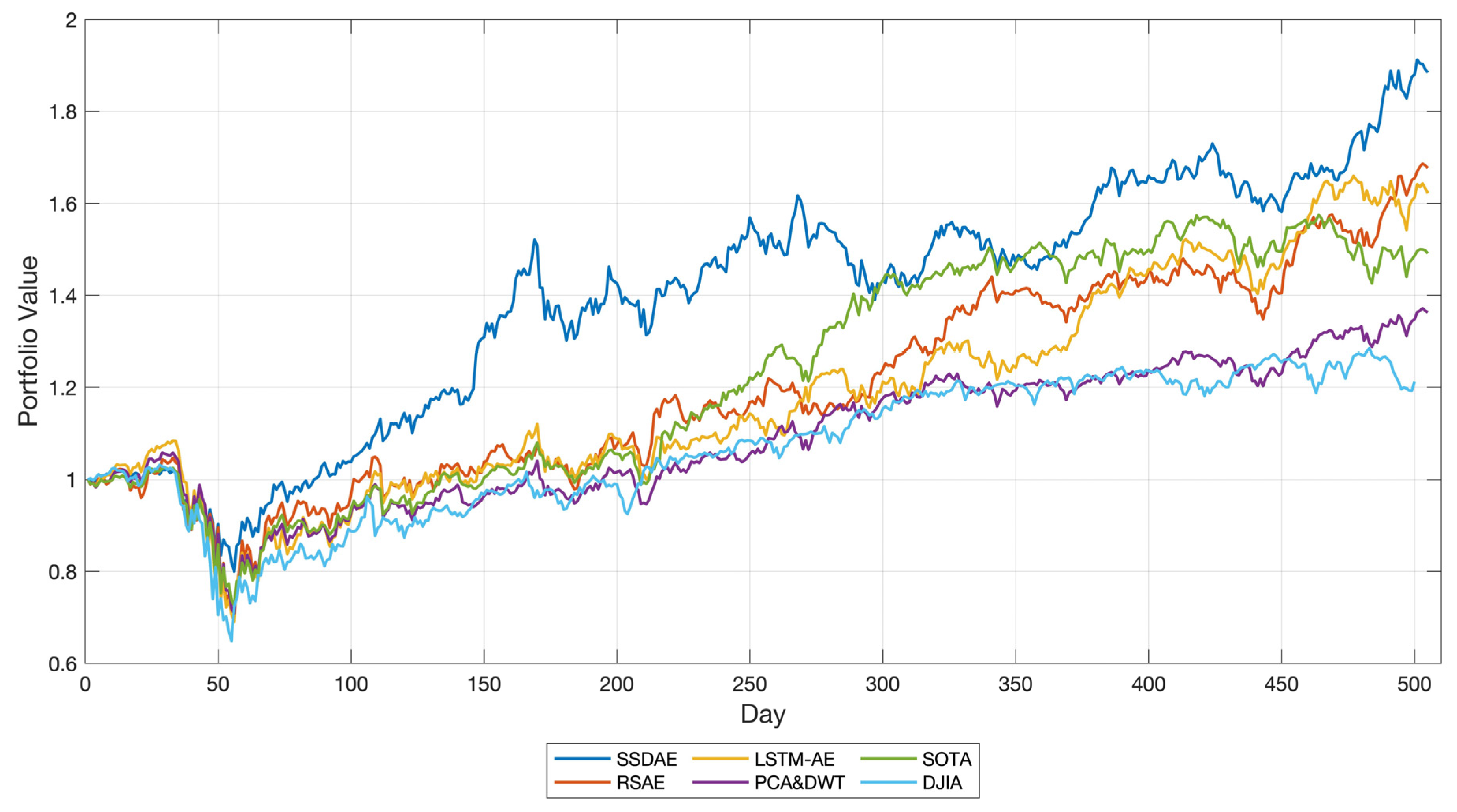
4.5. Results and Analysis
5. Conclusions
Author Contributions
Funding
Data Availability Statement
Acknowledgments
Conflicts of Interest
References
- Almahdi, S.; Yang, S.Y. An Adaptive Portfolio Trading System: A Risk-Return Portfolio Optimization Using Recurrent Reinforcement Learning with Expected Maximum Drawdown. Expert Syst. Appl. 2017, 87, 267–279. [Google Scholar] [CrossRef]
- Bertoluzzo, F.; Corazza, M. Testing Different Reinforcement Learning Configurations for Financial Trading: Introduction and Applications. Procedia Econ. Financ. 2012, 3, 68–77. [Google Scholar] [CrossRef]
- Deng, Y.; Bao, F.; Kong, Y.; Ren, Z.; Dai, Q. Deep Direct Reinforcement Learning for Financial Signal Representation and Trading. IEEE Trans. Neural Netw. Learn. Syst. 2017, 28, 653–664. [Google Scholar] [CrossRef] [PubMed]
- Fischer, T.G. Reinforcement Learning in Financial Markets—A Survey; FAU Discussion Papers in Economics: Erlangen, Germany, 2018. [Google Scholar]
- Jiang, Z.; Liang, J. Cryptocurrency Portfolio Management with Deep Reinforcement Learning. In Proceedings of the 2017 Intelligent Systems Conference (IntelliSys), London, UK, 7–8 September 2017; IEEE: New York, NY, USA, 2017; pp. 905–913. [Google Scholar]
- Zhang, Y.; Zhao, P.; Li, B.; Wu, Q.; Huang, J.; Tan, M. Cost-Sensitive Portfolio Selection via Deep Reinforcement Learning. IEEE Trans. Knowl. Data Eng. 2020, 34, 236–248. [Google Scholar] [CrossRef] [Green Version]
- Li, L. An Automated Portfolio Trading System with Feature Preprocessing and Recurrent Reinforcement Learning. arXiv 2021, arXiv:2110.05299. [Google Scholar]
- Qi, Y.; Wang, Y.; Zheng, X.; Wu, Z. Robust Feature Learning by Stacked Autoencoder with Maximum Correntropy Criterion. In Proceedings of the 2014 IEEE International Conference on Acoustics, Speech and Signal Processing (ICASSP), Florence, Italy, 4–9 May 2014; IEEE: New York, NY, USA, 2014; pp. 6716–6720. [Google Scholar]
- Li, W.; Shang, Z.; Gao, M.; Qian, S.; Zhang, B.; Zhang, J. A Novel Deep Autoencoder and Hyperparametric Adaptive Learning for Imbalance Intelligent Fault Diagnosis of Rotating Machinery. Eng. Appl. Artif. Intell. 2021, 102, 104279. [Google Scholar] [CrossRef]
- Jung, G.; Choi, S.-Y. Forecasting Foreign Exchange Volatility Using Deep Learning Autoencoder-LSTM Techniques. Complexity 2021, 2021, 6647534. [Google Scholar] [CrossRef]
- Yang, H.; Liu, X.-Y.; Zhong, S.; Walid, A. Deep Reinforcement Learning for Automated Stock Trading: An Ensemble Strategy. In Proceedings of the First ACM International Conference on AI in Finance, New York, NY, USA, 15–16 October 2020; pp. 1–8. [Google Scholar]
- García-Galicia, M.; Carsteanu, A.A.; Clempner, J.B. Continuous-Time Reinforcement Learning Approach for Portfolio Management with Time Penalization. Expert Syst. Appl. 2019, 129, 27–36. [Google Scholar] [CrossRef]
- Xu, K.; Zhang, Y.; Ye, D.; Zhao, P.; Tan, M. Relation-Aware Transformer for Portfolio Policy Learning. In Proceedings of the Twenty-Ninth International Conference on International Joint Conferences on Artificial Intelligence, Yokohama, Japan, 7–15 January 2021; pp. 4647–4653. [Google Scholar]
- Théate, T.; Ernst, D. An Application of Deep Reinforcement Learning to Algorithmic Trading. Expert Syst. Appl. 2021, 173, 114632. [Google Scholar] [CrossRef]
- Vincent, P.; Larochelle, H.; Bengio, Y.; Manzagol, P.-A. Extracting and Composing Robust Features with Denoising Autoencoders. In Proceedings of the 25th International Conference on Machine Learning, Helsinki, Finland, 5–9 July 2008; pp. 1096–1103. [Google Scholar]
- Hinton, G.E.; Osindero, S.; Teh, Y.-W. A Fast Learning Algorithm for Deep Belief Nets. Neural Comput. 2006, 18, 1527–1554. [Google Scholar] [CrossRef] [PubMed]
- Mohanty, D.K.; Parida, A.K.; Khuntia, S.S. Financial Market Prediction under Deep Learning Framework Using Auto Encoder and Kernel Extreme Learning Machine. Appl. Soft Comput. 2021, 99, 106898. [Google Scholar] [CrossRef]
- Bi, Q.; Yan, H.; Chen, C.; Su, Q. An Integrated Machine Learning Framework for Stock Price Prediction. In Proceedings of the China Conference on Information Retrieval, Xi’an, China, 14–16 August 2020; Springer: Cham, Switzerland, 2020; pp. 99–110. [Google Scholar]
- Bao, W.; Yue, J.; Rao, Y. A Deep Learning Framework for Financial Time Series Using Stacked Autoencoders and Long-Short Term Memory. PLoS ONE 2017, 12, e0180944. [Google Scholar] [CrossRef] [PubMed] [Green Version]
- Xu, Y.; Chhim, L.; Zheng, B.; Nojima, Y. Stacked Deep Learning Structure with Bidirectional Long-Short Term Memory for Stock Market Prediction. In Proceedings of the International Conference on Neural Computing for Advanced Applications, Shenzhen, China, 3–5 July 2020; Springer: Singapore, 2020; pp. 447–460. [Google Scholar]
- Gündüz, H. Stock Market Prediction with Stacked Autoencoder Based Feature Reduction. In Proceedings of the 2020 28th Signal Processing and Communications Applications Conference (SIU), Gaziantep, Turkey, 5–7 October 2020; IEEE: New York, NY, USA, 2020; pp. 1–4. [Google Scholar]
- Ross, S.; Mineiro, P.; Langford, J. Normalized Online Learning. arXiv 2013, arXiv:1305.6646. [Google Scholar]
- Zhang, Y.; Clavera, I.; Tsai, B.; Abbeel, P. Asynchronous Methods for Model-Based Reinforcement Learning. arXiv 2019, arXiv:1910.12453. [Google Scholar]
- Mnih, V.; Badia, A.P.; Mirza, M.; Graves, A.; Lillicrap, T.; Harley, T.; Silver, D.; Kavukcuoglu, K. Asynchronous Methods for Deep Reinforcement Learning. In Proceedings of the International Conference on Machine Learning, New York, NY, USA, 19–24 June 2016; pp. 1928–1937. [Google Scholar]
- Magdon-Ismail, M.; Atiya, A.F. Maximum Drawdown. Risk Mag. 2004, 17, 99–102. [Google Scholar]
- Sharpe, W.F. Mutual Fund Performance. J. Bus. 1966, 39, 119–138. [Google Scholar] [CrossRef]
- Young, T.W. Calmar Ratio: A Smoother Tool. Futures 1991, 20, 40. [Google Scholar]
- Brockman, G.; Cheung, V.; Pettersson, L.; Schneider, J.; Schulman, J.; Tang, J.; Zaremba, W. Openai Gym. arXiv 2016, arXiv:1606.01540. [Google Scholar]
- Soleymani, F.; Paquet, E. Financial Portfolio Optimization with Online Deep Reinforcement Learning and Restricted Stacked Autoencoder—DeepBreath. Expert Syst. Appl. 2020, 156, 113456. [Google Scholar] [CrossRef]
- Sun, H.; Rong, W.; Zhang, J.; Liang, Q.; Xiong, Z. Stacked Denoising Autoencoder Based Stock Market Trend Prediction via K-Nearest Neighbour Data Selection. In Proceedings of the International Conference on Neural Information Processing, Guangzhou, China, 14–18 November 2017; Springer: Cham, Switzerland, 2017; pp. 882–892. [Google Scholar]
- Jorion, P. Value at Risk: The New Benchmark for Managing Financial Risk; McGraw-Hill: New York, NY, USA, 2000. [Google Scholar]
- Rockafellar, R.T.; Uryasev, S. Conditional Value-at-Risk for General Loss Distributions. J. Bank. Financ. 2002, 6, 1443–1471. [Google Scholar] [CrossRef]


| Type | Financial Technical Indicators |
|---|---|
| Moving averages | Simple Moving Average (SMA) |
| Moving averages | The Exponential Moving Average (EMA) |
| Volatility | Average True Range (ATR) |
| Volatility | Williams Percent Range (WPR) |
| Trend | Moving Average Convergence Divergence (MACD) |
| Trend | Commodity Channel Index (CCI) |
| Momentum | Relative Strength Index (RSI) |
| Momentum | Awesome Oscillator (AO) |
| Momentum | TSI Indicator (TSI) |
| Volume | Force Index (FI) |
| Volume | On-Balance Volume (OBV) |
| Market | Start Date | End Date | Type |
|---|---|---|---|
| The US | 2014/01 | 2019/01 | Training set |
| 2019/01 | 2020/01 | Validation set | |
| 2020/01 | 2022/01 | Test set |
| Parameters | Value |
|---|---|
| trading window size (s) | 20 |
| risk-free rate of return A2C_learning_rate | 1% 0.0007 |
| A2C_ n_steps | 5 |
| Structure Parameters | Value | Learning Parameters | Value |
|---|---|---|---|
| Hidden layer 1 | 12 | Batch size | 100 |
| Hidden layer 2 | 9 | Epoch of pre-training | 50 |
| Hidden layer 3 | 6 | The sparsity | 10−8 |
| Hidden layer 4 | 3 | The regularization term | 10−5 |
Publisher’s Note: MDPI stays neutral with regard to jurisdictional claims in published maps and institutional affiliations. |
© 2022 by the authors. Licensee MDPI, Basel, Switzerland. This article is an open access article distributed under the terms and conditions of the Creative Commons Attribution (CC BY) license (https://creativecommons.org/licenses/by/4.0/).
Share and Cite
Yue, H.; Liu, J.; Tian, D.; Zhang, Q. A Novel Anti-Risk Method for Portfolio Trading Using Deep Reinforcement Learning. Electronics 2022, 11, 1506. https://doi.org/10.3390/electronics11091506
Yue H, Liu J, Tian D, Zhang Q. A Novel Anti-Risk Method for Portfolio Trading Using Deep Reinforcement Learning. Electronics. 2022; 11(9):1506. https://doi.org/10.3390/electronics11091506
Chicago/Turabian StyleYue, Han, Jiapeng Liu, Dongmei Tian, and Qin Zhang. 2022. "A Novel Anti-Risk Method for Portfolio Trading Using Deep Reinforcement Learning" Electronics 11, no. 9: 1506. https://doi.org/10.3390/electronics11091506