Efficient Colour Image Encryption Algorithm Using a New Fractional-Order Memcapacitive Hyperchaotic System

Abstract

In comparison with integer-order chaotic systems, fractional-order chaotic systems exhibit more complex dynamics. In recent years, research into fractional chaotic systems for the utilization of image cryptosystems has become increasingly highlighted. This paper describes the development, testing, numerical analysis, and electronic realization of a fractional-order memcapacitor. Then, a new four-dimensional (4D) fractional-order memcapacitive hyperchaotic system is suggested based on this memcapacitor. Analytically and numerically, the nonlinear dynamic properties of the hyperchaotic system have been explored, where various methods, including equilibrium points, phase portraits of chaotic attractors, bifurcation diagrams, and the Lyapunov exponent, are considered to demonstrate the chaos behaviour of this new hyperchaotic system. Consequently, an encryption cryptosystem algorithm is used for colour image encryption based on the chaotic behaviour of the memcapacitive model, where every pixel value of the original image is incorporated in the secret key to strengthen the encryption algorithm pirate anti-attack robustness. For generating the keyspace of that employed cryptosystem, the initial condition values, parameters, and fractional-order derivative value(s) (q) of the memcapacitive chaotic system are utilized. The common cryptanalysis metrics are verified in detail by histogram, keyspace, key sensitivity, correlation coefficient values, entropy, time efficiency, and comparisons with other recent related fieldwork in order to demonstrate the security level of the proposed cryptosystem approach. Finally, images of various sizes were encrypted and recovered to ensure that the utilized cryptosystem approach is capable of encrypting/decrypting images of various sizes. The obtained experimental results and security metrics analyses illustrate the excellent accuracy, high security, and perfect time efficiency of the utilized cryptosystem, which is highly resistant to various forms of pirate attacks.

1. Introduction

Multimedia, especially images, are one of the most essential information types nowadays, and they are simpler to obtain than in the past, thanks to the prevalence of smart technologies [1]. However, when these images must be transferred (exchanged) over different channels, security concerns arise, especially if any of them contain private information, such as military, national defence, legal concerns, and medicine applications [2,3].

The chaotic systems provide highly pseudorandom sequences with extreme entropy and low correlation between pixels in the encrypted image [4]. Matthews, a British scientist, proposed the first chaotic-based cryptosystem [5]. Due to the strength of the key generated using chaotic systems, a chaos-based cryptosystem has created a wide gap between the plain image and its consistent encrypted image, making this system difficult for intruders and attackers to recover the encrypted images [6].

Memcapacitor systems are a new family of memory-enabled circuit elements that accompany memristor systems. Chua proposed a different family of new circuit elements in the late 1970s and was one of the four guests in talks at the European Conference on Circuit Theory and Design in 1978 (ECCTD) [7]. A hysteretic loop, which may or may not intersect with the origin, is the most distinguishing feature [8]. The memristor has been used in a range of memcapacitor-based design application fields, including neuromorphic constructions, processer systems, and digital circuits, due to its particular properties [9].

Fractional calculus has recently gained a lot of attention since it provides more accurate models than integer-order calculus [10]. Fractional calculus may be used to describe many systems in transdisciplinary areas [11]. Fractional calculus is being employed in various areas of engineering and sciences, such as circuit theory, bioengineering, oscillators, viscoelasticity, electronics, chemistry, robotics, signal processing, and control theory [12]. Fractional-order chaotic models have additional complex dynamical behaviours compared with integer models because they include the fractional-order derivative value(s) parameter as well as the original system properties. This makes them beneficial in cryptosystems and secure communication protocols [13].

Recently, many image cryptosystem techniques based on chaotic systems have been developed for the public. In 2022, Qiang Lai et al. introduced a new memristive neuron model with hyperchaotic behaviours, where this new model has been employed for developing an image encryption scheme [14]. A new Hopfield neural network (HNN) based on a new memristor was designed by Qiang Lai et al. in 2022 [15]. That HNN was applied to investigate a new image encryption system. In 2021, Duzhong Zhang et al. proposed a hyperchaotic system-based image encryption scheme, where they employed transformed zigzag diffusion and ribonucleic acid (RNA) operation in this work [16]. Three-dimensional chaotic maps and reconstruction techniques have been used by Xiaoliang Qian et al. for suggesting a novel colour image encryption algorithm [17]. Noura Khalil et al. introduced an efficient chaos-based colour/grayscale image encryption scheme, where they used hyperchaotic maps that were considered in this article [18]. Lin Teng et al. presented a colour image encryption scheme based on a nonlinear discrete cross 2D chaotic map, wherein this algorithm combined cycle shift scrambling and selecting diffusion was utilized [19]. Shixu Li et al. established an image encryption scheme based on the fractional-order Lorenz system for encrypting colour images [20,21]. Our proposed cryptosystem was compared with these literature methods as summarized in

Table 1. Comparison metrics of our cryptosystem with similar works in the topic area.

Algorithm	Keyspace	NPCR	UACI	Horizontal rxy	Vertical rxy	Diagonal rxy	H(s)	Time Efficiency
Ref. [14]	2256	0.99602	0.3348	0.0019	0.0069	0.0087	7.9976	N/A
Ref. [15]	N/A	0.99602	0.3348	0.0019	0.0069	0.0087	7.9976	N/A
Ref. [16]	2256	0.99661	0.33617	0.0046	0.0024	0.0051	7.9973	28.49 s
Ref. [17]	2600	0.99690	0.33437	0.0004	0.0019	0.0012	N/A	N/A
Ref. [18]	2262	0.99620	0.33560	0.0023	0.0012	0.0001	7.9994	N/A
Ref. [19]	N/A	0.99643	0.33502	0.000617	0.000535	0.000411	7.9914	0.8379 s
Ref. [20]	2279	0.99613	0.334706	0.000312	0.002088	0.001444	7.9976	1.708 s
Ours	2744	0.99814	0.336251	0.000262	0.000472	0.00013	7.9996	0.45 s

.

According to this comparison, it is clear that the keyspace of our cryptosystem has high precision and is large enough to stick up to statistical attack. Additionally, it can be observed from Table 1 that the NPCR and UACI results of the proposed cryptosystem are quite near the ideal (theoretical) values, and the cryptosystem is effective against both plaintext and differential attacks. Additionally, the employed algorithm is better than all mentioned algorithms in the light of correlation coefficients and information entropy. Furthermore, the results of the security analysis and comparisons exposed that our proposed cryptosystem not only has high-security performance, but also has speed advantage compared with other related works, where it has encryption/decryption time faster than other literature encryption algorithms.

In our article, we suggest a new 3D fractional-order memcapacitive hyperchaotic- oscillator that contains a single unstable equilibrium. A fractional-order memcapacitor has been developed, experienced, numerically simulated, and electronically realized. Then, this fractional-order memcapacitor is considered for constructing the objected fractional-order memcapacitive hyperchaotic oscillator.

Furthermore, experiments such as phase portraits of chaotic attractors, system equilibria, bifurcation diagrams, and Lyapunov exponents are explored to demonstrate the proposed memcapacitive hyperchaotic system’s complex dynamical chaotic behavior. Moreover, the new fractional-order memcapacitive hyperchaotic system was utilized for developing an efficient image cryptosystem. Additionally, histogram, keyspace, key sensitivity, entropy, time efficiency, correlation coefficient, and comparisons with similar fieldwork are used to display the cryptanalysis metrical tests in detail in order to approve the security strength of the employed encryption approach and its robustness resistance against different attacks. Finally, images of various sizes and extensions were encrypted and recovered to demonstrate that the proposed cryptosystem approach was capable of encrypting/decrypting images of various sizes. MATLAB was used to validate our work, testing, and results.

The remainder of this article is organized as follows: In Section 2, a brief basic knowledge of fractional-order systems is reviewed. Section 3 presents an investigation of the developed fractional-order memcapacitor model, testing and electronically realizing that memcapacitor and fixing its parameters, and the charge–voltage characteristic curve was obtained in this section. A new fractional-order memcapacitive hyperchaotic oscillator based on that established fractional-order memcapacitor is designed in Section 4, and also, the system equilibria and its chaotic attractors are discussed in this section. As presented in Section 5, bifurcation diagrams and Lyapunov exponents are used to display the dynamical behavior properties of the proposed hyperchaotic system.

The details of our suggested image cryptosystem technique are presented in Section 6. Experimental results and some common security cryptoanalysis metrics of the employed cryptosystem are given in Section 7 and Section 8, respectively. In Section 9, the conclusions of this paper are offered.

2. Mathematical Preliminaries

The concept of a noninteger (fractional order) derivative was first introduced in a letter from Leibniz to L’Hospital in 1695 [22]. Recently, many different relations of fractional-order derivative and integral operators have been discovered to be very significant and productive owing to their proven applicability in a wide range of fields. Many of these fractional-order operators offer fascinating and actually useful tools for solving ordinary and partial differential equations, as well as integral, integrodifferential equations and differintegral equations [23]. They are fractional-calculus equivalents and extensions of each of these equations and a variety of other problems involving special functions of applied mathematics and mathematical physics, as well as their extensions and generalities in one or further variables. Riemann–Liouville, Grünwald–Letnikov, and Caputo are three of the most popular fractional-order operators in the fractional-order calculations [24].

The fractional calculus is based on generalizing integration and differentiation to any order, which can be integer, noninteger (fractional), and complex. The fundamental continuous differintegral operator with order value (q) was created as a result of this generalization, as described by the following Equation (1) [25]:

$$t_0{D}_t^{q}f\left(t\right)=\{\begin{array}{c}\frac{d^{k}f\left(t\right)}{d{t}^k}q>0\\ 1q=0\\ \underset{0}{\overset{t}{{\displaystyle \int }}}{\left(f\left(\tau \right)\right)}^{-q}d\tau q<0\end{array}$$

(1)

Generally, in the fractional calculus, the gamma function, symbolized as Γ(.), is the essential function, as specified in Equation (2) [26]:

$$\Gamma \left(n\right)={{\displaystyle \int }}_0^{+\infty }{e}^{-t}{t}^{n-1}dt ;n>0; \Gamma \left(1\right)=1, \Gamma \left(0\right)=+\infty$$

(2)

Riemann–Liouville acquired a fractional-order integral operator (J^q) in 1847, which is defined as follows [27]:

$$J^{q}f\left(t\right)=\{\begin{array}{c}\frac{1}{\Gamma \left(q\right)}\underset{0}{\overset{t}{{\displaystyle \int }}}{\left(t-\tau \right)}^{q-1}f\left(t\right)d\tau ; q<0\\ f\left(t\right) ; q=0.\end{array}$$

(3)

where q represents the fractional-order value.

The Grünwald–Letnikov derivative is a fundamental fractional extension of the natural derivative. Anton Karl Grünwald introduced it in 1867, followed by Aleksey Vasilievich Letnikov in 1868. It was written like this [28]:

$$D^{q}x\left(t\right)=f\left(x,t\right)=\underset{h\to 0}{lim}{h}^{-q}\left(-1\right){\displaystyle \sum }_{j=0}^{t/h}\left(-1\right)\left(\begin{array}{c}q\\ j\end{array}\right)x\left(t-jh\right)$$

(4)

where h denotes the step size.

Caputo introduced a mathematical model for a fractional-order derivative of a function f(t), which is specified as follows in Equation (5) [29]:

$$t_0{D}_t^{q}f\left(t\right)=\{\begin{array}{c}\frac{1}{\Gamma \left(k-q\right)}\underset{t_0}{\overset{t}{{\displaystyle \int }}}\frac{f^{\left(k\right)}\left(\tau \right)}{{\left(t-\tau \right)}^{q-k+1}}d\tau ; k-1<q<k\\ \frac{d^{k}f\left(t\right)}{d{t}^k} ; q=k.\end{array}$$

(5)

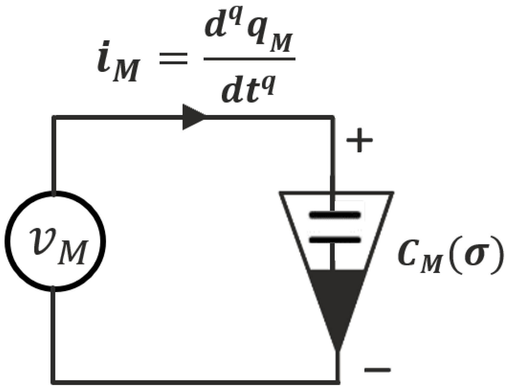
3. Memcapacitor Model

A memcapacitor is a type of memristive system whose features are defined by a relationship between the flux time integral (φ(t)) and the charge time integral (σ(t)) [30]. In 2009, the concept of memristor was extended to memcapacitor, as well as by Di Ventra et al., where memcapacitor is defined as [31]:

$$\begin{array}{c}\begin{array}{c}{q}_M\left(t\right)=C_M\left(\sigma ,v_M,t\right)v_M\left(t\right)\\ \dot{\sigma }=f\left(\sigma ,v_M,t\right)\end{array}\\ \begin{array}{c}{v}_M\left(t\right)=C_M^{-1}\left(\sigma ,q_M,t\right)q_M\left(t\right)\\ \dot{\sigma }=f\left(\sigma ,q_M,t\right)\end{array}\end{array}$$

(6)

where $q_M$ represents the quantity of the charge passing through the memcapacitor at time t, $v_M$ is the consistent voltage across the memcapacitor, $\dot{\sigma }$ signifies the memcapacitor internal state variable, and $C_M$ and $C_M^{-1}$ denote the meme capacitance and memcapacitance inverse, respectively. The memcapacitor model can be simplified in terms of the flux time integral and the charge time integral as follows:

$$\begin{array}{c}{q}_M\left(t\right)=C_M[\underset{t_0}{\overset{t}{{\displaystyle \int }}}{v}_M\left(\tau \right)d\tau ]v_M\left(t\right)=C_M\left[\phi \left(t\right)\right]v_M\left(t\right)\\ v_M\left(t\right)=C_M^{-1}[\underset{t_0}{\overset{t}{{\displaystyle \int }}}{q}_M\left(\tau \right)d\tau ]q_M\left(t\right)=C_M^{-1}\left[\sigma \left(t\right)\right]q_M\left(t\right)\end{array}$$

(7)

Equation (7) demonstrates the memcapacitors in terms of voltage-controlled and charge-controlled memcapacitors. The charge-controlled memcapacitor model is the common useful model, and it is simply described by the following Equation (8) [32]:

$$\begin{array}{c}{v}_M\left(t\right)=C_M^{-1}\left(\sigma \left(t\right),q_M\left(t\right)\right)\\ \dot{\sigma }\left(t\right)=q_M\left(t\right)\end{array}$$

(8)

3.1. Integer-Order Situation

An integer voltage-controlled memcapacitor that is modelled in [21] and presented as in Equation (9) is used for designing a memcapacitive hyperchaotic system:

$$\begin{array}{c}{v}_M\left(t\right)=\left(\alpha +\beta \left|\sigma \left(t\right)\right|\right)q_M\left(t\right)\\ \dot{\sigma }\left(t\right)=q_M\left(t\right)\end{array}$$

(9)

where the memcapacitance inverse in Equation (9) is described by $C_M^{-1}=\left(a+b \left|\sigma \left(t\right)\right|\right)$. Consequentially, the initial values of the memcapacitance and its variation in terms of charge going through it are represented by α and β, respectively. Generally, α and β are known as the memcapacitor parameters or constant coefficients. The memcapacitor parameters can be customized to meet the needs of the memcapacitor state. Here, these parameters are selected as α = −0.75 and β = 1.72. The memcapacitor hysteresis loop characteristics of $q_M-v_M$ are shown in Figure 1 when the excitation signal is the memcapacitor charge, which is sinusoidal as presented below by the following Equation (10):

$$q_M\left(t\right)=A_{M}cos\left(2\pi ft\right)$$

(10)

In Equation (10), A_M and f present memcapacitor charge amplitude and its frequency, respectively. The $q_M-v_M$ hysteresis loop characteristics of the memcapacitor specified in Figure 1 are obtained with different values of amplitudes and frequencies.

3.2. Fractional-Order Situation

The memcapacitor values vary depending on the internal state variable and the behavior of the hysteresis loop of the memcapacitor model. The internal states of the charge-controlled memcapacitor display noticeable memory properties, and the relationship between charge and the voltage represents the mentioned hysteresis loop. Therefore, the fractional charge-controlled memcapacitor corresponding to model (9) was designated as in the following equation:

$$\begin{array}{c}{v}_M\left(t\right)=\left(\alpha +\beta \left|\sigma \left(t\right)\right|\right)q_M\left(t\right)\\ \frac{d^q\sigma }{d{t}^q}=q_M\left(t\right)\end{array}$$

(11)

In the above Equation (11), the symbol q signifies the fractional-order derivative value of the internal memcapacitor state (σ(t)). Here, it is necessary to distinguish the fractional-order derivative value signified by the q symbol and the symbol $q_M$ that represents the quantity of the charge pass through the memcapacitor. With the identical values of parameters selected in the above integer memcapacitor case, the $q_M-v_M$ hysteresis loop characteristics of the fractional-order memcapacitor were obtained as illustrated in Figure 2. The amplitudes and frequencies of the injected charge are 10 C and 1 Hz, respectively, and different fractional-order derivative values (q).

3.3. Electronic Circuit of the Fractional-Order Memcapacitor

An electronic circuit realization of that fractional memcapacitor confirms the practicality of using that fractional memcapacitor in real-world applications. According to Equation (9), the realization of that memcapacitor can be validated using traditional operational amplifiers for conducting the mathematical functions in this equation, such as inverting arrangement, gain arrangement, integer integrator arrangement, and weighted summer arrangement. Consequently, for realizing the memcapacitor in the fractional case, however, the integer integrator arrangement must be substituted with a fractional-order arrangement, as exposed in Equation (11). In other words, a fractional-order integrator can be built using a traditional integer integrator arrangement by substituting the capacitor with a fractance related to the required fractional order.

A fractance is a fractional-order impedance electrical component. Based on the conventional description of the fractional differintegral, the fractional operators cannot be directly implemented in time-domain simulations. To investigate such systems, approximations to fractional functions using regular integer-order functions can be considered. According to circuit theory, the fractance equivalent circuit’s complex frequency domain can accomplish fractional-order approximation formulation (q-order). The fractional order was employed (q = 0.99), and the approximation of 1/s^0.99 can be derived using Equation (12) [33]:

$$\frac{1}{s^{0.99}}=\frac{1.1370\left(s+10.355\right)\left(s+11103.4\right)}{\left(s+0.0104\right)\left(s+11.1034\right)\left(s+11906\right)}$$

(12)

where Equation (12) can be constructed using chain fractance made up of three pairs of resistor capacitor, as shown in Figure 3:

Therefore, a transfer function between the chain fractance terminals (A and B), which is illustrated in Figure 3, can be calculated using Equation (13).

$$\begin{gathered} H_{0.99}\left(s\right)=\frac{1/C_1}{\left(s+1/R_{f1}{C}_1\right)}+\frac{1/C_2}{\left(s+1/R_{f2}{C}_2\right)}+\frac{1/C_3}{\left(s+1/R_{f3}{C}_3\right)} \\ =\frac{1}{C_0}\left[\frac{\left(\frac{C_0}{C_1}+\frac{C_0}{C_2}+\frac{C_0}{C_3}\right)\left(s^2+\left(\frac{\left(\frac{c_2+c_3}{R_{f1}}+\frac{c_1+c_3}{R_{f2}}+\frac{c_1+c_2}{R_{f3}}\right)}{c_1{c}_2+c_2{c}_3+c_1{c}_3}\right)S+\left(\frac{\left(\frac{R_{f1}+R_{f2}+R_{f3}}{R_{f1}{R}_{f2}{R}_3}\right)}{c_1{c}_2+c_2{c}_3+c_1{c}_3}\right)\right)}{\left(1+1/R_{f1}{C}_1\right)\left(1+1/R_{f2}{C}_2\right)\left(1+1/R_{f3}{C}_3\right)}\right] \end{gathered}$$

(13)

In Equation (13), C₀ signifies a unit limit, choosing Co = 1 µF and H_0.99(s)·C₀ = 1/s^0.99. These electronic component properties result from using Equations (12) and (13), where the comparison was used. Thus, the values of the resistors R_f1, R_f2, and R_f3 were obtained to be 95.082 MΩ, 6.441 kΩ, and 6.436 kΩ, respectively, while the values of the capacitors C₁, C₂, and C₃ were calculated to be 13.982, 13.05, and 1.011 μF, as illustrated in Figure 3.

The chain fractance scheme shown in Figure 3 has been employed to substitute the capacitor in the standard integer integrator arrangement to accomplish the fractional integration with order derivative value (q = 0.99). As a result, based on the fractional-order memcapacitor described by Equation (11), the fractional-order memcapacitor circuit has been modelled to be as described by the fowling Equation (14):

$$\begin{array}{c}{v}_M\left(t\right)=\left(\frac{R_5}{R_6}\alpha +\frac{R_5}{R_4} \left|\sigma \left(t\right)\right|\right)q_M\left(t\right)\\ \dot{\sigma }\left(t\right)=\frac{1}{R_1{C}_{eq}}{q}_M\left(t\right)\end{array}$$

(14)

In Equation (14), C_eq is the fractional-order impedance comparable to the fractance cell, and it corresponds to proving the fractional integrator with order value (q = 0.99). As a result, the equivalent electronic circuit consistent with Equation (14) has been realized as illustrated in Figure 4.

By applying a charge with 10 C amplitude, 1 Hz frequency, and 0.99 fractional derivative value of the fractional-order memcapacitor, the $q_M-v_M$ characteristic curve is obtained, as displayed in Figure 5. The electronic circuit of the fractional-order memcapacitor is realized using Multisim. The figurative scheme of a fractional-order memcapacitor is shown in Figure 6.

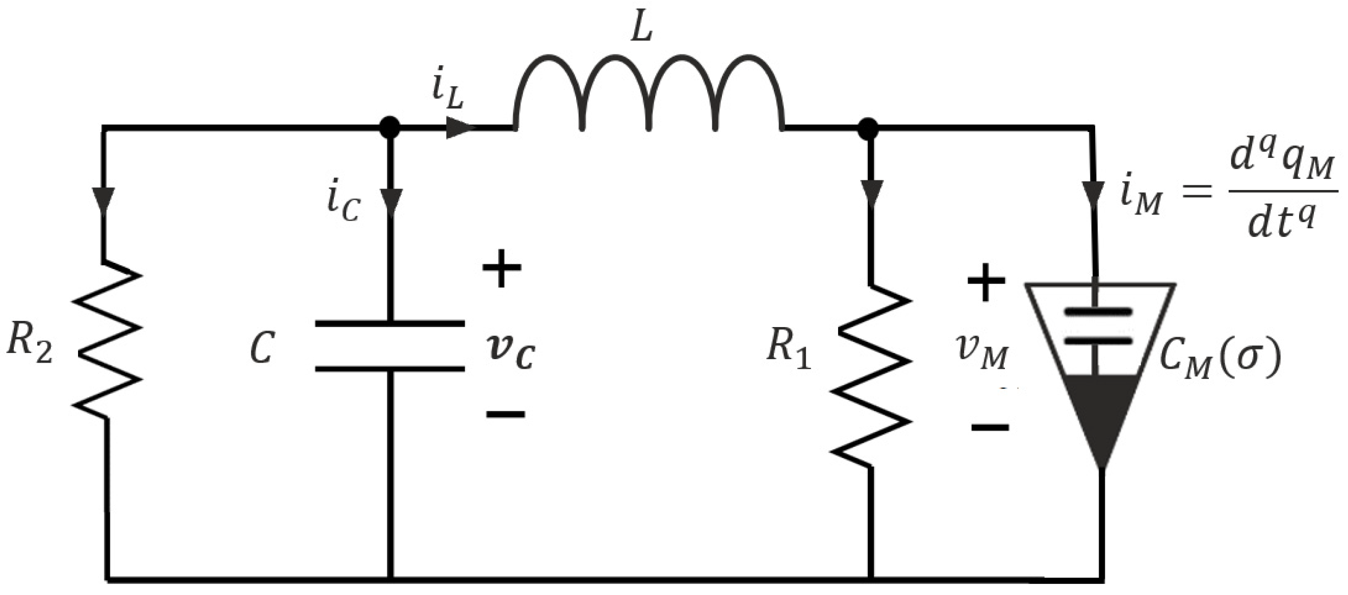
4. Fractional-Order Memcapacitive-Based Chaotic Circuit

Because the limited hysteresis loop or recall of prior states is an important aspect of the memcapacitor, chaotic circuits containing memristors must be evaluated using a method that considers memory effects and provides more degrees of freedom for analysis. In this work, a fractional-order memcapacitive chaotic circuit with the fractional-order memcapacitor modelled by Equation (11) is proposed. Figure 7 depicts the proposed fractional-order memcapacitive chaotic circuit.

By applying Kirchhoff’s current law to the circuit in Figure 7, the fractional-order memcapacitor’s state equations are determined as follows:

$$\begin{gathered} L\frac{d^q{i}_L}{d{t}^q}=v_{C }-v_{M } \\ C\frac{d^q{v}_C}{d{t}^q}=-i_L-\frac{v_{C }}{R_{2 }} \\ {i}_{M }=i_L-\frac{v_{C }}{R_{1 }} \end{gathered}$$

(15)

Then, by replacing the voltage $\left(v_{M }\right)$ of and the internal state $(\dot{\mathsf{\sigma }}\left(t\right))$ of the fractional-order memcapacitor designated by Equation (11) in Equation (15), the dynamics of the proposed fractional-order memcapacitive chaotic system can be calculated using Equation (16):

$$\begin{gathered} \frac{d^q{i}_L}{d{t}^q}=\frac{1}{L}\left(v_{C }-\left(\alpha +\beta \left|\sigma \left(t\right)\right|\right)q_M\left(t\right)\right) \\ \frac{d^q{v}_C}{d{t}^q}=\frac{1}{C}\left(-i_L-\frac{v_C}{R_2}\right) \\ \frac{d^q{q}_M}{d{t}^q}=i_L-\frac{\left(\alpha +\beta \left|\sigma \left(t\right)\right|\right)q_M\left(t\right)}{R_1} \\ \frac{d^q\sigma }{d{t}^q}=q_M\left(t\right) \end{gathered}$$

(16)

Dimensionless dynamics can be found for the fractional-order memcapacitive chaotic model defined by Equation (16) as follows. Let $i_L=x$, $v_C=y$, $q_M=z$, σ = u, 1/L = a, 1/C = b, 1/R₁ = d, and 1/R₂ = g; thus, the fractional-order memcapacitive chaotic model can be defined as:

$$\begin{gathered} \frac{d^{q}x}{d{t}^q}=a\left(y-\left(\alpha +\beta \left|u\right|\right)z\right) \\ \frac{d^{q}y}{d{t}^q}=b\left(-x-gy\right) \\ \frac{d^{q}z}{d{t}^q}=i_L-d\left(\alpha +\beta \left|u\right|\right)z \\ \frac{d^{q}u}{d{t}^q}=z \end{gathered}$$

(17)

where a, b, d, g, α, and β signify the parameter, while x, y, z, and u represent the state variables and the fractional-order derivative value symbolized by q.

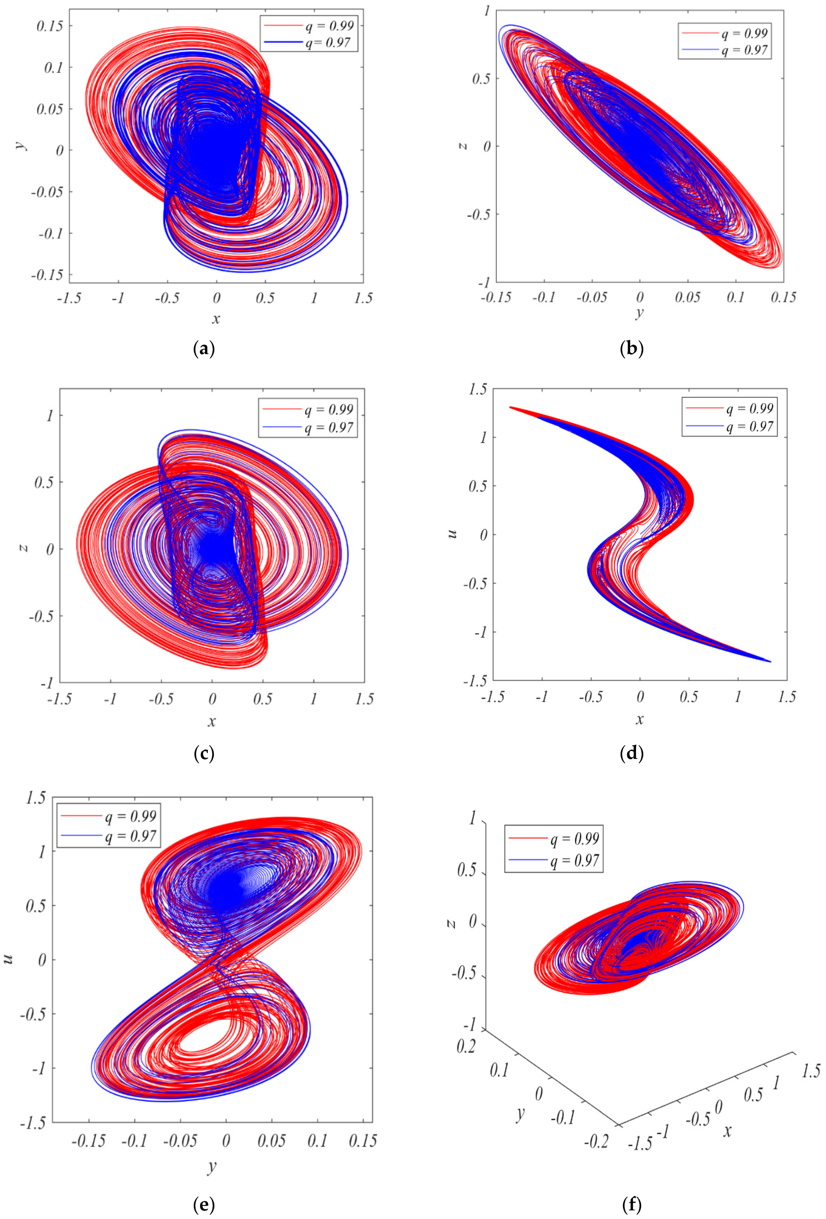
4.1. Chaotic Behaviours of the Memcapacitive System

The proposed fractional-order memcapacitive system modelled by Equation (17) can exhibit chaotic behaviours when its parameters are selected to be a = 2.2222, b = 0.1667, d = 0.45, g = 2, α = −0.75, and β = 1.72. That system is numerically simulated with initial conditions (x₀, y₀, z₀, u₀) = (0.001, 0, 0, 0) and two different fractional-order derivative values (q = 0.97 and q = 0.99). Figure 8 depicts the phase portrait attractors of a fractional-order memcapacitive chaotic model (17) consistent with these designated setting values. A layout of phase portrait chaotic attractors is showed in two-dimensional (2D) and three-dimensional (3D) topologies.

4.2. Equilibria and Stability

Simply, the fractional-order memcapacitive-based basic chaotic system’s equilibria (equilibrium or fixed points) can be computed by setting the state equations of the system (17) to be zero as follows:

$$\begin{gathered} \frac{d^{q}x}{d{t}^q}=a\left(y-\left(\alpha +\beta \left|u\right|\right)z\right)=0 \\ \frac{d^{q}y}{d{t}^q}=b\left(-x-gy\right)=0 \\ \frac{d^{q}z}{d{t}^q}=x-d\left(\alpha +\beta \left|u\right|\right)z=0 \\ \frac{d^{q}u}{d{t}^q}=z=0 \end{gathered}$$

(18)

By solving the system (18), it is clear that the fractional-order memcapacitive chaotic model (17) contains only one equilibrium point, which is (x*, y*, z*, u*) = (0, 0, 0, 0). The Jacobian matrix will be used for determining the stability of the system equilibrium points, where the following highlighted Theorem 1 is used:

Theorem 1.

Consider the following fractional-order system described by the following Equation (19) [34]:

$$\frac{d^{q}x\left(t\right)}{d{t}^q}=f\left(x\left(t\right)\right)$$

(19)

The equilibrium points of$f\left(x\left(t\right)\right)$are locally asymptotically stable if all eigenvalues λ_i (i = 1, 2, 3…, n) of the Jacobian matrix $J=\partial f\left(x\left(t\right)\right)/ \partial x\left(t\right)$ evaluated at the equilibrium points satisfy $\left|arg\left({\lambda }_i\right)\right|>q\frac{\pi }{2}$.

By the linearizing approach, we gained the Jacobian matrix of the system (17), as described by the following Equation (20):

$$J=\left[\begin{array}{cccc}0& a& -a\left(\alpha -\beta \left|u\right|\right)& -a\beta zsgn\left(u\right)\\ -b& -bg& 0& 0\\ 1& 0& -d\left(\alpha -\beta \left|u\right|\right)& -d\beta zsgn\left(u\right)\\ 0& 0& 1& 0\end{array}\right]$$

(20)

As defined by following Equation (21), the Jacobian calculation consistent with the evaluated equilibrium point P(0,0,0,0) was computed.

$$J_{E\left(0,0,0,0\right)}=\left[\begin{array}{cccc}0& a& -a\alpha & 0\\ -b& -bg& 0& 0\\ 1& 0& -d\alpha & 0\\ 0& 0& 1& 0\end{array}\right]$$

(21)

The system parameters were used as a = 2.2222, b = 0.1667, d = 0.45, g = 2, α = −0.75, and β = 1.72. Therefore, the eigenvalues corresponding to the matrix described by Equation (21) were calculated as (λ₁ = 0, λ_2,3 = −0.6926 ± 0.1105i, and λ₄ = 1.3668). Based on Theorem 1, it’s clear that the fractional-order derivative value (q) limits the stability of the equilibrium point. Because we used fractional derivative order value (q = 0.99) in this study, the first and fourth eigenvalues have |arg(λ_1,4)|= 0. That indicates that the stability condition specified in Theorem 1 was not obeyed. Therefore, the equilibrium point P(0,0,0,0) is classified as an unstable equilibrium point. As a result, an excitation from this unstable equilibrium point P(0,0,0,0) might be used to generate a self-excited attractor. As a result, the suggested fractional-order memcapacitive system defined by Equation (17) is excited by this equilibrium point, which is accountable for its chaotic performance.

5. Dynamic Analysis

In this section, for investigating the nonlinear dynamics of the advised fractional-order memcapacitive chaotic model defined by Equation (17), bifurcation analysis and Lyapunov exponents are used.

5.1. Bifurcation Diagrams

When one or more system parameters are slightly changed, bifurcation diagrams are a valuable tool for evaluating system behavior. It can also be used to figure out various system properties, such as the path to chaos [35]. In this work, the effect of a slight change in the α parameter of the system (17) is explored to show the nonlinear dynamics behavior when a slight change occurs in this parameter, where α is plotted in contradiction to the system state variable x(t) as exposed in Figure 9. Furthermore, the system state variable x(t) is plotted versus the system fractional-order derivative value (q), employing bifurcation diagrams to investigate the system’s nonlinear dynamics. The bifurcation illustration, shown in Figure 10, was used to demonstrate the impact of the fractional-order derivative value on the dynamical behaviour of the system. The bifurcation diagrams in Figure 9 and Figure 10 are exposed with initial conditions (x₀, y₀, z₀, u₀) being (0.001,0,0,0), with the system (17) parameters and fractional-order derivative value (q) as shown in

Table 2. The system (17) parameters and fractional-order derivative value (q) utilized in examination bifurcation diagrams (Figure 9 and Figure 10).

Figure 9		Figure 10
Parameter	Value	Parameter	Value
a	2.2222	a	2.2222
b	0.1667	b	0.1667
d	0.45	d	0.45
g	2	g	2
α	Variable	α	0.75
β	1.72	β	1.72
Fractional-order (q)	0.99	Fractional-order (q)	Variable

.

As shown in Figure 9, the suggested model displays chaotic performance when the system parameter α is slightly changed. Additionally, as demonstrated in the bifurcation diagram in Figure 10, the system (17) can also stimulate chaotic performance when the model fractional-order derivative value is more than 0.985 (q > 0.985).

As shown in Figure 9 and Figure 10, the suggested fractional-order memcapacitive chaotic system given by Equation (17) exhibits various bifurcation topological patterns.

These findings indicate that a new fractional-order memcapacitive chaotic model can generate chaotic action. In this work, the bifurcation diagrams in Figure 9 and Figure 10 were plotted using Roberto Garrappa’s procedure with a step of size (h = 0.005) and an advanced code that we wrote [36].

5.2. Lyapunov Exponents

In nonlinear systems, Lyapunov exponents were computed and powerfully verified that our new system can display chaotic behaviours [37]. The Lyapunov exponents (Lei; I = 1, 2, …, n) represent the exponential attraction or time leave taking of two adjacent orbits in the phase space. An n-dimensional system has n Lyapunov exponents [38]. When the system contains at least one (at least) positive Lyapunov exponent, the system is said to be in a chaotic system [39]. Consequently, a system that exhibits chaotic behavior with at least two positive Lyapunov exponents is often defined as a hyperchaotic system.

In this work, the Lyapunov exponents are exposed in two arrangements. In the first Lyapunov exponent investigation, the Lyapunov exponents are considered with respect to the time as illustrated in Figure 11. The numerical investigation of the constructed system’s Lyapunov exponents is obtained over a simulation time of 500 s, where the settling values the Lyapunov exponents as Le1 = 0.0291, Le2 = 0.0035, Le3 = −0.006, and Le4 = −0.211. The presence of two positive Lyapunov exponents (Le3 and Le4) is plenty to prove that the system (17) is a hyperchaotic system.

In the second Lyapunov exponent investigation, Lyapunov exponents are measured in contradiction to changing the fractional-order derivative value (q), where q ∈ [0.98,1], as presented in Figure 12. The settling values of Lyapunov exponents were obtained to be Le1 = 0.0317, Le2 = 0.0174, Le3 = −0.0187, and Le4 = − 0.1071.

It is clear in Figure 11 and Figure 12 that the proposed fractional-order memcapacitive system named by Equation (17) is capable of exhibiting chaotic dynamics behaviours, and it is a hyperchaotic system. Figure 11 and Figure 12 are numerically exposed to initial conditions (x₀, y₀, z₀, u₀) being (0.001, 0, 0, 0), with the system (17) parameters and fractional-order derivative value (q) as shown in

Table 3. The system (17) parameters utilized in examination Lyapunov exponents.

Figure 11		Figure 12
Parameter	Value	Parameter	Value
a	2.2222	a	2.2222
b	0.1667	b	0.1667
d	0.45	d	0.45
g	2	g	2
α	0.75	α	0.75
β	1.72	β	1.72
Fractional-order (q)	0.99	Fractional-order (q)	Variable

.

6. Image Encryption Algorithm

Chaotic encryption algorithms have been successfully utilized to encrypt a variety of images, ranging from remote sensing to medical and elsewhere. In this part, we present an image cryptosystem technique that uses the fractional-order memcapacitive hyperchaotic system defined by Equation (14). This system produces chaotic signals (x, y, z, and u). By integrating these obtained chaotic sequences with the plain image pixels, we will encrypt and decrypt an image. Figure 13 describes the overall encryption operations.

The encryption algorithm in the proposed chaotic-based cryptosystem is described in full below:

Step 1. 

Read a coloured plain image to obtain its pixel values as a matrix I_M*N, where M and N represent the rows and columns of the image pixels, respectively.

Step 2. 

Decompose this image into its three basic bands, which are R (red), G (green), and B (blue).

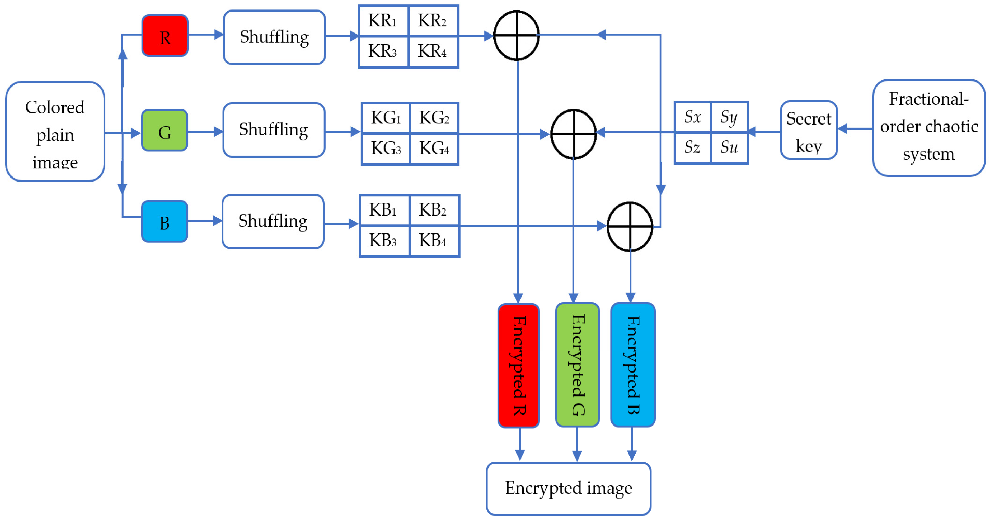
Step 3. 

Read these three bands, R, G, and B, to obtain their pixel values as matrices IR_M*N, IG_M*N, and IB_M*N, respectively. Then shuffle these three matrixes, where the histogram will remain unchanged, whereas it will be further difficult for an intruder to decode the image unless he knows the specific shuffling procedure.

Step 4. 

Each shuffled pixel matrix of the bands R, G, and B is split to four nonoverlapped submatrices (KP₁, KP₂, KP₃, KP₄; P = R,G,B), as shown in Figure 13. In other words, the original band matrix is divided into four blocks, taking into account the total number of elements in the obtained four submatrices equivalent to the pixel number of the basic band matrix. The size of these submatrices is determined as follows:

Size(KP₁) = Round(M/2) × round(N/2)

Size(KP₂) = Round(M/2) × floor(N-N/2)

Size(KP₃) = Floor (M-M/2) × round(N/2)

Size(KP₄) = Floor (M-M/2) × floor(N-N/2)

Step 5. 

For the fractional-order memcapacitive hyperchaotic system defined by Equation (17), set the following values: initial conditions (x₍₀₎, y₍₀₎, z₍₀₎, u₍₀₎), fractional-order derivative value (q), and parameters, which are a, b, d, g, α, and β.

Step 6. 

Use these determined values in step 5 for simulating the fractional-order memcapacitive hyperchaotic system (17). Consequently, iterate the solving process with fixed steps to ensure the iteration solution set coverage of the submatrix size of the generated chaotic sequence for each state variable (x, y, z, and u). Then randomly select elements from the solution set for each state variable of the system (17) with a number equivalent to the decomposed four blocks in step 4, where x, y, z, and u state variables are responsible for generating matrices with element numbers equivalent to these four blocks, KP₁, KP₂, KP₃, and KP₄, respectively.

Step 7. 

To determine the secret keys S_x,y,z,u, preprocess the chaotic sequences of the state_. variables obtained in step 6. The following mathematical operations are used to obtain these secret keys:

$$\begin{gathered} S_{xi}=\left|round\left(mod\left(\left|(x_i-floor\left(\left|x_i\right|\right)\right|\right)\ast 5\ast {10}^5\right),256))\right|; i \\ =1, 2,\dots , Round\left(M/2\right)round\left(N/2\right). \end{gathered}$$

$$\begin{gathered} S_{yi}=\left|round\left(mod\left(\left|(y_i-floor\left(\left|y_i\right|\right)\right|\right)\ast 5\ast {10}^5\right),256))\right|; i \\ =1, 2,\dots ,Round\left(M/2\right)floor\left(N-N/2\right). \\ {S}_{zi}=\left|round\left(mod\left(\left|(z_i-floor\left(\left|z_i\right|\right)\right|\right)\ast 5\ast {10}^5\right),256))\right|;i \\ =1,2,\dots ,Floor\left(M-M/2\right)round\left(N/2\right). \\ {S}_{ui}=\left|round\left(mod\left(\left|(u_i-floor\left(\left|u_i\right|\right)\right|\right)\ast 5\ast {10}^5\right),256))\right|; i \\ =1, 2,\dots ,Floor\left(M-M/2\right)floor\left(N-N/2\right). \end{gathered}$$

Step 8. 

Reshape these obtained secret keys in step 7 to form the matrices S_x, S_y, S_z, and S_u, where their sizes as round(M/2) × round(N/2), round(M/2) × floor(N-N/2), floor(M-M/2) × round(N/2), and floor(M-M/2) × floor(N-N/2), respectively.

Step 9. 

Encrypt the pixels in the four blocks of each band (R, G, and B) of the plain image using the obtained secret key in step 8 by the flowing operations:

$$\begin{gathered} E_{R1}=K{R}_1\oplus S_x; E_{R2}=K{R}_2\oplus S_y; E_{R3}=K{R}_3\oplus S_z; E_{R4}=K{R}_4\oplus S_u \\ {E}_{G1}=K{G}_1\oplus S_x; E_{G2}=K{G}_2\oplus S_y; E_{G3}=K{G}_3\oplus S_z; E_{G4}=K{G}_4\oplus S_u \\ {E}_{B1}=K{B}_1\oplus S_x; E_{B2}=K{B}_2\oplus S_y; E_{B3}=K{B}_3\oplus S_z; E_{B4}=K{G}_4\oplus S_u \end{gathered}$$

where $\oplus$ signifies the B-XOR operation, and E_{Ri(i = 1,2,3,4)}, E_{Gi(i = 1,2,3,4)}, and E_{Bi(i = 1,2,3,4)} are the encrypted blocks of the R, G, and B bands, respectively.

Step 10. 

Rearrange (reshape) these encrypted blocks obtained in step 9 to form the encrypted matrix bands (encrypted R, encrypted G, and encrypted B) of the original image.

Step 11. 

Recompose the encrypted bands obtained in step 10 to give the encrypted image corresponding to the coloured plain image.

Consequently, the decryption technique is an exact inverse operation of the encryption procedure in order to restore the original image, as illustrated in Figure 14. Because we employed a symmetric key encryption algorithm, the cryptosystem sides (source and destination) can use a secret approach to exchange encryption/decryption keys. There are a number of common means for doing this, including saving the encryption/decryption keys beforehand and exchanging them over a secret channel or a disguised trusted postman.

7. Experimental Results

In this section, a “Lena.png” colour plain image of size 512 × 512 was experimentally tested, where this image was encrypted and decrypted using the proposed hyperchaotic-based cryptosystem. That was performed to demonstrate the feasibility and efficiency of the proposed hyperchaotic-based cryptosystem.

In this test, the parameters of the fractional-order hyperchaotic system were given values as a = 2.2222, b = 0.1667, d = 0.45, g = 2, α = −0.75, and β = 1.724 with initial conditions (x₀, y₀, z₀, u₀) = (0.001, 0, 0, 0) and a fractional-order derivative value (q = 0.99). The system (17) was numerically solved with iterations, which ensures that the number of solution sets of the total state variables (x, y, z, and u) can cover 262,144 samples. These samples match the whole number of pixels in the original image (MN = 512 × 512).

Then from these obtained solution sets, 65,536 (MN/4) samples were chosen for each state variable (x, y, z, and u) to create a chaotic sequence that is responsible for secret key matrices (S_x, S_y, S_z, and S_u) highlighted in step 7 (Section 6). Figure 15 displays the visual investigation of the employed hyperchaotic-based cryptosystem on a “Lena.png” colour plain image of size 512 × 512. Figure 15a displays the plain image. R, G, and B bands of the original image are illustrated in Figure 15b–d, respectively. On the other hand, the encrypted (ciphered) images of the respective original R, G, and B are exposed in Figure 15e,f. The recovered (decrypted) images corresponding to the encrypted images are displayed in Figure 15i–l in their respective arrangements. As can be seen in Figure 15, it demonstrates the exact identicalness between the plain and recovered image, which shows the high accuracy of the proposed cryptosystem in recovering the original images. Furthermore, the encrypted images are wholly different from their respective plain images, and these images do not display any pattern similar to the plain images. As a result, the attacker will be unable to extract any information or patterns from the encrypted images. That shows the robust resistance of the cryptosystem against attacks.

8. Cryptanalysis

The performance efficiency of the suggested hyperchaotic-based image cryptosystem is evaluated in this section utilizing several security test methods. A good cryptosystem, as is well known, should exhibit very robust resistance to different attacks and high sensitivity to the key(s) and contain a great plenty of keyspace to thwart adventurer attempts [40]. Here, the following common metrics were explored: histogram, key sensitivity, information entropy, correlation coefficients of adjacent pixels, time efficiency, and other common metrics used to evaluate the efficiency of the image cryptosystems.

8.1. Histogram Check

Generally, the histograms are used to count and plot the spreading of an image’s pixel values (pixel brightness levels). Since the colour image contains three bands (R, B, and B) and each band is an 8-bit image, the original colour image can be considered a 24-bit image. Thus, there are 256 (2⁸) different possible brightnesses of each of these three bands, which are from 0 to 255. As a result, the histogram will display 256 numbers representing the distribution of the image pixels signifying their intensity levels [41]. The histogram of an encrypted image must be statistically and visually dissimilar from the histogram of the plain image. In order to resist statistical pirate attacks, the histogram of the encrypted image and its R, G, and B bands must have a reasonably consistent (flat) shape. The flatness of the histogram specifies the randomness of the encrypted image pixel values. Figure 16a displays the histograms of the plain colour Lena image. Figure 16b–d displays the histogram of the R, G, and B bands of the plain Lena image. On the other hand, the histograms of the encrypted images of the respective original Lena, R, G, and B are shown in Figure 16e,f. The recovered images consistent with the encrypted images are shown in Figure 16i–l in their respective arrangements.

As exposed in Figure 16, it can be understood that the encrypted image histograms have a significantly different distribution compared with the original image’s histograms, and that the encrypted image’s pixel intensities have a uniform distribution (flat), demonstrating that the proposed cryptosystem algorithm offers excellent robustness to statistical attacks. In other words, the encrypted image’s histograms are equally distributed. As a result, the encrypted images offer no information about the original images. Furthermore, the histogram distribution of the recovered image in Figure 16e–h is exactly similar to that of the plain image histogram in Figure 16i–l, respectively. As a result, the plain image can be successfully retrieved with perfect accuracy.

8.2. Keyspace Analysis

The keyspace in any cryptosystem is a significant facet of the security when a pirate force assault takes place [42]. The secret keys are generated in our work by suggesting the fractional-order memcapacitive hyperchaotic system termed by Equation (17). Therefore, the secret keys include the system (17) initial condition values (x₍₀₎, y₍₀₎, z₍₀₎, u₍₀₎), parameters (a, b, d, g, α, and β), and fractional-order derivative value (q).

Fractional-order chaotic systems, as highlighted in the introduction section, are extremely sensitive to slight variations in the fractional-order derivative value (q), the system parameters, and the initial conditions. Assuming that each employed key takes 10⁻¹⁵ step alteration, then the whole keyspace is computed to be (10¹⁶)¹⁴ = 10²²⁴ ≈ 2⁷⁴⁴. These findings indicate that the keyspace of the utilized encryption approach is large enough to resist all forms of brute force attacks.

8.3. Key Sensitivity Analysis

In any cryptosystems, extreme key sensitivity is required for verifying highly secure encryption methods, which means that the ciphered image cannot be recovered successfully even if the encryption and decryption keys are only slightly changed [43]. The robust encryption algorithm should be extremely sensitive to any slight variations in the secret (encryption/decryption) keys. This guarantees the safety of the cryptosystem approach against brute force attacks. In this work, the system (17) initial condition values (x₀, y₀, z₀, u₀), its parameters (a, b, d, g, α, and β), and the fractional-order derivative value (q) control the sensitivity of the secret keys in the employed cryptosystem approach.

Generally, the key sensitivity is determined by computing the net pixel change rate (NPCR) and the unified average changing intensity (UACI). These values compute the influence of little variations in the secret keys for retrieving the plain image. Higher NPCR and UACI ratings mean that the encryption method is very resistant to various pirate attacks [44].

The NPCR calculates the percentage change of the pixel number alteration degree between two images. UACI, on the other hand, calculates the average brightness of the differences between the two images. The following Equations (22) and (23) can be used to compute the NPCR and UACI, respectively [45]:

$$NPCR=\frac{{{\displaystyle \sum }}_{i=1}^M {{\displaystyle \sum }}_{j=1}^N\left|sign\left(I\left(i,j\right)-D\left(i,j\right)\right)\right|}{M·N}\times 100\%$$

(22)

$$UACI=\frac{1}{255}\frac{{{\displaystyle \sum }}_{i=1}^M {{\displaystyle \sum }}_{j=1}^N\left|I\left(i,j\right)-D\left(i,j\right)\right|}{M·N}\times 100\%$$

(23)

In Equation (22), M × N grants image size, I(i, j) presents plain image, D(i, j) presents recovered image, (i, j) grants pixel image location, and if I(i, j) ≠ D(i, j),|sign(⋅)| =1; otherwise, |sign(⋅)| = 0. In the experimental test, the secret keys S_x,y,z,u are created based on the solution set of the system (17) with the chosen parameters a = 2.2222, b = 0.1667, d = 0.45, g = 2, α = −0.75, and β = 1.724 with initial conditions (x₀, y₀, z_0, u₀) = (0.001, 0, 0, 0) and fractional-order derivative value (q = 0.99), where a 512 × 512 color “Lena.png” plain image is encrypted by these keys. Consequently, in the decryption procedure, just the fractional-order derivative value (q) was very slightly varied as q = 0.99 + 10⁻¹⁵ in NPCR and UACI tests for determining key sensitivity.

Table 4. Key sensitivity analysis.

Direction	Original Images
	Lena	R Band	G Band	B Band
NPCR	0.99814	0.99783	0.9982	0.99813
UACI	0.33625	0.336192	0.33626	0.33620

illustrates the results of key sensitivity comparative assessments of NPCR and UACI. Furthermore, Figure 17 depicts the experimental results of a recovering image with the aforementioned very little variation at the decryption key.

These findings imply that the original image cannot be retrieved by utilizing the incorrect keys (even if they varied very slightly somewhat from the original key). As a result, the proposed cryptosystem based on the fractional-order memcapacitive hyperchaotic system (17) is extremely sensitive to secret keys, and it is also effective for resisting brute force attacks.

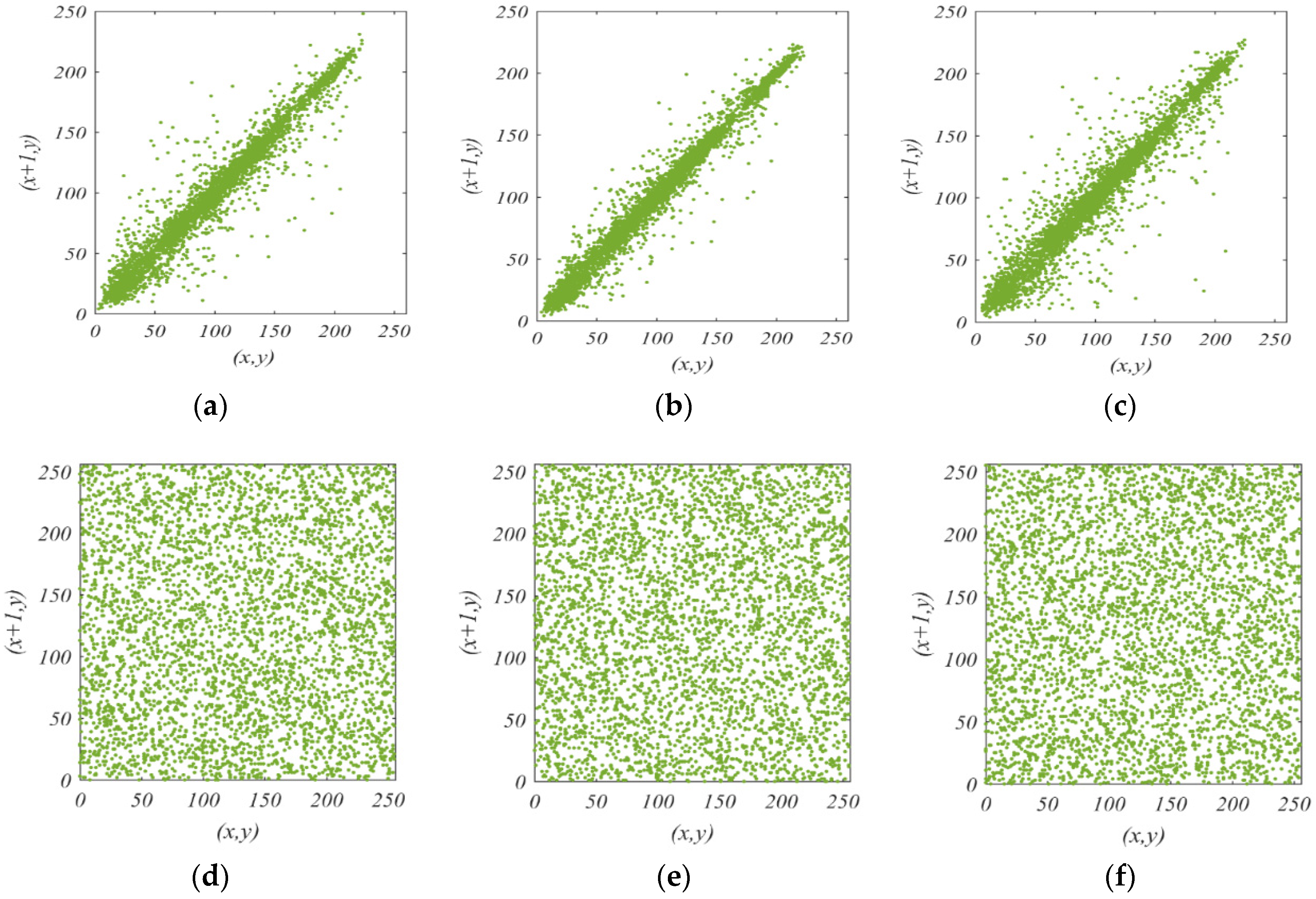
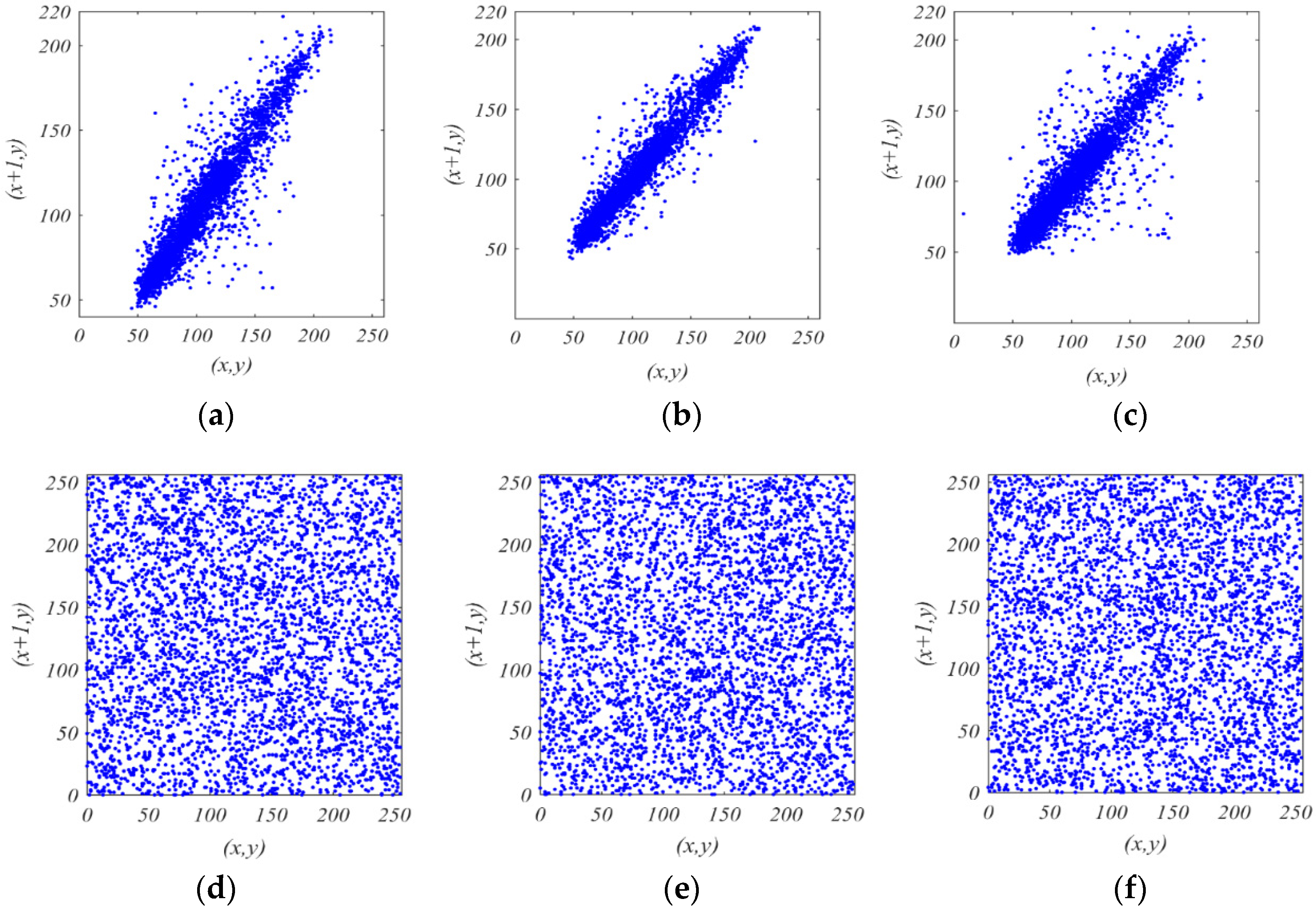
8.4. Correlation Coefficients Analysis

The correlation coefficients are calculated by comparing the values of two adjacent pixels, and they are used to measure data randomness of the encrypted images. Two head-to-head pixels in the original image are significantly connected to each other. However, for the encrypted image, this number should be as low as feasible, meaning the lowest possible correlation between two neighbouring pixels. A high-security image encryption system must be capable of diminishing the correlation between the neighbouring pixels of an encrypted image. In other words, the cryptosystem’s security is inversely related to the correlation coefficient scores obtained [46].

Commonly, correlation coefficient values are computed for a specific number of adjacent pixels in horizontal arrangement (H), vertical arrangement (V), and diagonal arrangement (D).

In an image, the correlation coefficients of two head-to-head pixel x, y values are computed as follows [47]:

$$r_{xy}=\frac{cov\left(x,y\right)}{\sqrt{D\left(x\right)}\sqrt{D\left(y\right)}}$$

(24)

In Equation (24), x and y signify the two neighbouring pixel values, cov(x, y) presents the covariance function, and D(.) denotes the variance. The values cov(x, y) and D(.) can be computed as in the following Equations (25) and (26), respectively [48]:

$$cov\left(x,y\right)=\frac{{{\displaystyle \sum }}_{i=1}^N \left(x_i-E\left(x\right)\right)\left(x_i-E\left(y\right)\right)}{N}$$

(25)

$$D\left(k\right)=\frac{{{\displaystyle \sum }}_{i=1}^N {(k_i-E\left(k\right))}^2}{N}$$

(26)

where the whole number of selected pixels in the image was symbolled by N in Equation (22), and the average is E(k), which can be calculated by Equation (27) as in the following:

$$E\left(k\right)=\frac{{{\displaystyle \sum }}_{i=1}^N k_i}{N}$$

(27)

In our work, for the correlation confection computation, we arbitrarily chose 4000 pairings of adjacent pixels from the plain and its encrypted images in vertical, horizontal, and diagonal arrangements.

Table 5. Correlation coefficients of the proposed cryptosystem.

Direction	Plain Images				Encrypted Images
	Lena	R Band	G Band	B Band	Lena	R Band	G Band	B Band
Vertical	0.9821	0.9712	0.9677	0.9675	0.000472	0.000466	0.000413	0.000398
Horizontal	0.9743	0.9638	0.9847	0.9789	0.000262	0.000269	0.000245	0.000221
Diagonal	0.9672	0.9855	0.9789	0.9813	0.00013	0.000157	0.000173	0.000141

shows the gained correlation confections of adjacent pixels for the plain image and its consistent encrypted image.

Table 5 shows that the plain image pixels have a very robust correlation, while the encrypted image pixels have an actual low correlation, demonstrating that the utilized cryptosystem approach is quite robust for resisting brute force attacks.

Moreover, Figure 18 displays the correlation coefficient plots of the plain Lena image and its consistent encrypted image in horizontal, vertical, and diagonal orders. Consequently, the correlation coefficient plots of the R of the plain Lena image and its corresponding encrypted R band are visibly illustrated in Figure 19. Figure 20 depicts the correlation coefficient plots of the G band of the plain Lena image and its equivalent encrypted G band. On the other hand, the B band of the plain image and its consistent B encrypted band are demonstrated in Figure 21.

It can be seen from Figure 18, Figure 19, Figure 20 and Figure 21 that the plain image and its R, G, and B bands show a very weighty correlation of the related pixels. In other words, as illustrated in Figure 18a–c, Figure 19a–c, Figure 20a–c and Figure 21a–c, all of the pixel points in the plain image and its R, G, and B bands are concentrated along with the diagonal alliance. On the other hand, as shown Figure 18d–f, Figure 19d–f, Figure 20d–f and Figure 21d–f, the responded encrypted image pixel dots are distributed across the whole entire plane. This verifies that the correlations between various pixels in the encrypted image have significantly lessened. The ability to change closely related pixels of a plain image into unrelated pixels of an encrypted image is a desirable feature of an encryption method. As a result, the encrypted image has a lot more randomness, which makes statistical analysis difficult for attackers. This demonstrates that the employed cryptosystem based on a fractional-order memcapacitive system offers great security effectiveness.

8.5. Entropy Evolution

The entropy of an image determines the distribution of its pixel values between 0 and 255 [49]. It determines the degree of unpredictability and ambiguity in the image. The perfect theoretical rate of information entropy in the encrypted image is 8 because each of the 256 intensity levels of a pixel image is specified by 8 bits. Practically, the encrypted image’s information entropy value should be closer as possible to 8. Equation (28) expresses the entropy of information as follows [50]:

$$H\left(s\right)={\displaystyle \sum }_{i=1}^{255} p(s_i)lo{g}_2\left(\frac{1}{p(s_i)}\right)$$

(28)

In Equation (28), p(.) signifies the pixel value probability.

Table 6. Entropy evaluations of the employed cryptosystem.

	Original Image	Encrypted Image
Lena	7.2351	7.9996
R Band	7.1334	7.9994
G Band	6.9541	7.9995
B Band	7.1263	7.9993

presents the computed entropy evaluations of the plain color (Lena image) and its R, G, and B bands and their equivalent encrypted images, respectively.

As can be seen from Table 6, wholly, the encrypted image’s entropy evaluations are quite close to the theoretical perfect (ideal) value. As a result, our cryptosystem provides robust resistance to entropy attacks.

8.6. Time Efficiency

The time efficiency of any cryptosystem algorithm is a significant metric for evaluating the performance of the cryptosystem. The maximum duration of time it could take for any algorithm to accomplish a computational task with perfect precision can be defined as execution time [51]. A real cryptosystem must have excellent encryption/decryption speeds as well as its high-security function. In this article, for the colour plain “Lena.png” image of size 512 × 512, the average time efficiency of the utilized encryption/decryption procedure is 0.5 s. These findings specify the advantages of the used cryptosystem technique in items of speed efficacy.

8.7. Comparison with Related Works

As is well known, any work should be compared with similar works in the topic area in order to demonstrate the developed work’s performance efficiency. In order to demonstrate the high-performance efficiency and security of the proposed fractional-order memcapacitive hyperchaotic system described by Equation (17) in an image encryption application, we compare our obtained findings with other highlighted works in the introduction section for metrics of the employed cryptanalysis tests.

Table 1 displays a comparison for the encrypted image, where the best values for the cryptanalysis test coefficients were chosen from the publications that were compared. In summary, the image encryption approach based on the new fractional-order memcapacitive hyperchaotic system (17) demonstrates an excellent encryption result, a high level of security, and perfect time efficiency, as shown in Table 1.

Finally, the colour “macaws.jpg” with a size of 300 × 309 and “fruits.bmp” with a size of 236 × 235 were encrypted and recovered. This was revealed in order to test the effectiveness of the cryptosystem algorithm employed to encrypt and recover various-sized images and different extensions. The plain image, encrypted image, and recovered image of the macaws are shown in Figure 22a–c, correspondingly. Consequently, Figure 22d–f shows the histogram graphs that correspond to Figure 22a–c, respectively. Figure 23a–c shows the original image, its consistent encrypted image, and the corresponding recovered image of the fruits, correspondingly. Figure 23d–f shows the histogram graph that corresponds to Figure 23a–c.

9. Conclusions

In this article, a fractional-order memcapacitor was developed, numerically investigated, and electronically realized. Then this fractional-order memcapacitor was employed for suggesting a novel fractional-order memcapacitive chaotic oscillator. To demonstrate the nonlinear dynamical performances of this system, the chaotic attractors, equilibrium point, bifurcation maps, and Lyapunov exponents were examined analytically and numerically. According to the dynamic analysis, the new fractional-order memcapacitive chaotic system is extremely sensitive to slight changes in parameters, initial conditions, and its fractional-order derivative values. As a result, the system produces chaotic sequences with a high randomness degree. Consequently, it has been employed in a cryptosystem approach for encrypting color plain images. The initial conditions, state variables, parameters, and fractional-order derivative values of the memcapacitive chaotic system were used to produce the keyspace of the proposed cryptosystem. In order to confirm the security strength of the proposed cryptosystem algorithm, the common cryptanalysis metrics were explored in detail, including keyspace analysis, histogram analysis, key sensitivity, entropy analysis, correlation coefficients, time efficiency examination, and comparisons with articles in a comparable topic area. The obtained values of the investigated cryptanalysis metrics were as keyspace = 2⁷⁴⁴, NPCR = 0.99814, UACI = 0.336251, H(s) = 7.9996, and time efficiency = 0.45 s. The acquired experimental findings and detailed security assessments support the utilized cryptosystem’s effectiveness, high-level security, and good time efficiency, and show high robust resistance to various types of attacks.

References

1. Shirmohammadi, S.; Ferrero, A. Camera as the instrument: The rising trend of vision based measurement. IEEE Instrum. Meas. Mag. 2014, 17, 41–47. [Google Scholar] [CrossRef]
2. Ghadirli, H.M.; Nodehi, A.; Enayatifar, R. An overview of encryption algorithms in color images. SSignal Process. 2019, 164, 163–185. [Google Scholar] [CrossRef]
3. Li, Z.; Peng, C.; Tan, W.; Li, L. A novel chaos-based image encryption scheme by using randomly DNA encode and plaintext related permutation. Appl. Sci. 2020, 10, 7469. [Google Scholar] [CrossRef]
4. Kaur, M.; Singh, S.; Kaur, M.; Singh, A.; Singh, D. A Systematic Review of Metaheuristic-based Image Encryption Techniques. Arch. Comput. Methods Eng. 2021, 1–15. [Google Scholar] [CrossRef]
5. Rahman, Z.-A.S.A.; Jasim, B.H.; Al-Yasir, Y.I.A.; Abd-Alhameed, R.A. High-Security Image Encryption Based on a Novel Simple Fractional-Order Memristive Chaotic System with a Single Unstable Equilibrium Point. Electronics 2021, 10, 3130. [Google Scholar] [CrossRef]
6. Qiang, L.; Wan, Z.; Kamdem Kuate, P.D. Modelling and circuit realization of a new no-equilibrium chaotic system with hidden attractor and coexisting attractors. Electron. Lett. 2020, 56, 1044–1046. [Google Scholar]
7. Wang, G.; Jiang, S.; Wang, X.; Shen, Y.; Yuan, F. A novel memcapacitor model and its application for generating chaos. Math. Probl. Eng. 2016, 2016, 1–15. [Google Scholar] [CrossRef]
8. Patil, S.R.; Chougale, M.Y.; Rane, T.D.; Khot, S.S.; Patil, A.A.; Bagal, O.S.; Jadhav, S.D.; Sheikh, A.D.; Kim, S.; Dongale, T.D. Solution-processable ZnO thin film memristive device for resistive random access memory application. Electronics 2018, 7, 445. [Google Scholar] [CrossRef] [Green Version]
9. Rahman, Z.-A.S.A.; Jasim, B.H.; Al-Yasir, Y.I.A.; Hu, Y.-F.; Abd-Alhameed, R.A.; Alhasnawi, B.N. A New Fractional-Order Chaotic System with Its Analysis, Synchronization, and Circuit Realization for Secure Communication Applications. Mathematics 2021, 9, 2593. [Google Scholar] [CrossRef]
10. Mainardi, F. Fractional calculus. In Fractals and Fractional Calculus in Continuum Mechanics; Springer: Vienna, Austria, 1997; pp. 291–348. [Google Scholar]
11. Liao, T.-L.; Chen, H.-C.; Peng, C.-Y.; Hou, Y.-Y. Chaos-based secure communications in biomedical information application. Electronics 2021, 10, 359. [Google Scholar] [CrossRef]
12. Rahman, Z.-A.; Jasim, B.; Al-Yasir, Y.; Abd-Alhameed, R.; Alhasnawi, B. A New No Equilibrium Fractional Order Chaotic System, Dynamical Investigation, Synchronization, and Its Digital Implementation. Inventions 2021, 6, 49. [Google Scholar] [CrossRef]
13. Ye, G.; Jiao, K.; Wu, H.; Pan, C.; Huang, X. An asymmetric image encryption algorithm based on a fractional-order chaotic system and the RSA public-key cryptosystem. Int. J. Bifurc. Chaos 2020, 30, 2050233. [Google Scholar] [CrossRef]
14. Lai, Q.; Lai, C.; Zhang, H.; Li, C. Hidden coexisting hyperchaos of new memristive neuron model and its application in image encryption. Chaos Solitons Fractals 2022, 158, 112017. [Google Scholar] [CrossRef]
15. Lai, Q.; Wan, Z.; Zhang, H.; Chen, G. Design and analysis of multiscroll memristive hopfield neural network with adjustable memductance and application to image encryption. IEEE Trans. Neural Netw. Learn. Syst. 2022, 1–14. [Google Scholar] [CrossRef] [PubMed]
16. Zhang, D.; Chen, L.; Li, T. Hyper-chaotic color image encryption based on transformed zigzag diffusion and RNA operation. Entropy 2021, 23, 361. [Google Scholar] [CrossRef]
17. Qian, X.; Yang, Q.; Li, Q.; Liu, Q.; Wu, Y.; Wang, W. A novel color image encryption algorithm based on three-dimensional chaotic maps and reconstruction techniques. IEEE Access 2021, 9, 61334–61345. [Google Scholar] [CrossRef]
18. Khalil, N.; Sarhan, A.; Alshewimy, M.A. An efficient color/grayscale image encryption scheme based on hybrid chaotic maps. Opt. Laser Technol. 2021, 143, 107326. [Google Scholar] [CrossRef]
19. Teng, L.; Wang, X.; Yang, F.; Xian, Y. Color image encryption based on cross 2D hyperchaotic map using combined cycle shift scrambling and selecting diffusion. Nonlinear Dyn. 2021, 105, 1859–1876. [Google Scholar] [CrossRef]
20. Li, S.; Yu, Y.; Ji, X.; Sun, Q. A novel colour image encryption based on fractional order Lorenz system. Syst. Sci. Control Eng. 2020, 9, 141–150. [Google Scholar] [CrossRef]
21. Yuan, F.; Li, Y.; Wang, G.; Dou, G.; Chen, G. Complex dynamics in a memcapacitor-based circuit. Entropy 2019, 21, 188. [Google Scholar] [CrossRef] [Green Version]
22. Rahman, Z.; Jassim, B.; Al Yasir, Y. New Fractional Order Chaotic System: Analysis, Synchronization, and it’s Application. Iraqi J. Electr. Electron. Eng. 2021, 17, 116–123. [Google Scholar] [CrossRef]
23. Sabatier, J.; Agrawal, O.P.; Machado, J.A.T. Advances in Fractional Calculus; Springer: Dordrecht, The Netherland, 2007. [Google Scholar]
24. Baleanu, D.; Diethelm, K.; Scalas, E.; Trujillo, J.J. Fractional Calculus: Models and Numerical Methods; World Scientific: Singapore, 2012; Volume 3. [Google Scholar]
25. Ortigueira, M.D. Fractional Calculus for Scientists and Engineers; Springer Science & Business Media: Berlin, Germany, 2011; Volume 84. [Google Scholar]
26. Loverro, A. Fractional Calculus: History, Definitions and Applications for the Engineer. Available online: https://www.semanticscholar.org/paper/Fractional-Calculus-%3A-History-%2C-Definitions-and-for-Loverro/6256fee0c10bdb7096df51ca8e64df58414ed026 (accessed on 25 March 2022).
27. Abdon, A.; Gómez-Aguilar, J.F. Numerical approximation of Riemann-Liouville definition of fractional derivative: From Riemann-Liouville to Atangana-Baleanu. Numer. Methods Partial. Differ. Equ. 2018, 34, 1502–1523. [Google Scholar]
28. Srivastava, H.M. Fractional-order integral and derivative operators and their applications. Mathematics 2020, 8, 1016. [Google Scholar] [CrossRef]
29. Algahtani, O.J.J. Comparing the Atangana–Baleanu and Caputo–Fabrizio derivative with fractional order: Allen Cahn model. Chaos Solitons Fractals 2016, 89, 552–559. [Google Scholar] [CrossRef]
30. Ventra, M.D.; Pershin, Y.V.; Chua, L.O. Circuit elements with memory: Memristors, memcapacitors, and meminductors. Proc. IEEE 2009, 97, 1717–1724. [Google Scholar] [CrossRef] [Green Version]
31. Romero, F.; Ohata, A.; Toral-Lopez, A.; Godoy, A.; Morales, D.; Rodriguez, N. Memcapacitor and meminductor circuit emulators: A review. Electronics 2021, 10, 1225. [Google Scholar] [CrossRef]
32. Pu, Y.-F. Measurement units and physical dimensions of fractance-part II: Fractional-order measurement units and physical dimensions of fractance and rules for fractors in series and parallel. IEEE Access 2016, 4, 3398–3416. [Google Scholar] [CrossRef]
33. Akgul, A. Chaotic oscillator based on fractional order memcapacitor. J. Circuits Syst. Comput. 2019, 28, 1950239. [Google Scholar] [CrossRef]
34. Hosseinnia, S.H.; Ghaderi, R.; Mahmoudian, M.; Momani, S. Sliding mode synchronization of an uncertain fractional order chaotic system. Comput. Math. Appl. 2010, 59, 1637–1643. [Google Scholar] [CrossRef] [Green Version]
35. Rahman, Z.-A.S.A.; Al-Kashoash, H.A.A.; Ramadhan, S.M.; Al-Yasir, Y.I.A. Adaptive control synchronization of a novel memristive chaotic system for secure communication applications. Inventions 2019, 4, 30. [Google Scholar] [CrossRef] [Green Version]
36. Garrappa, R. Numerical solution of fractional differential equations: A survey and a software tutorial. Mathematics 2018, 6, 16. [Google Scholar] [CrossRef] [Green Version]
37. Jasim, B.H.; Hassan, K.H.; Omran, K.M. A new 4-D hyperchaotic hidden attractor system: Its dynamics, coexisting attractors, synchronization and microcontroller implementation. Int. J. Electr. Comput. Eng. 2021, 11, 2068–2078. [Google Scholar] [CrossRef]
38. Jasim, B.H.; Mjily, A.H.; Al-Aaragee, A.M.J. A novel 4 dimensional hyperchaotic system with its control, synchronization and implementation. Int. J. Electr. Comput. Eng. 2021, 11, 2974–2985. [Google Scholar] [CrossRef]
39. Al-Hussein, A.-B.; Tahir, F.; Ouannas, A.; Sun, T.-C.; Jahanshahi, H.; Aly, A. Chaos suppressing in a three-buses power system using an adaptive synergetic control method. Electronics 2021, 10, 1532. [Google Scholar] [CrossRef]
40. Akhavan, A.; Samsudin, A.; Akhshani, A. Cryptanalysis of an image encryption algorithm based on DNA encoding. Opt. Laser Technol. 2017, 95, 94–99. [Google Scholar] [CrossRef]
41. Moussa, K.H.; Naggary, A.I.E.; Mohamed, H.G. Non-linear hopped chaos parameters-based image encryption algorithm using histogram equalization. Entropy 2021, 23, 535. [Google Scholar] [CrossRef]
42. Xiang, Y.; Xiao, D.; Zhang, R.; Liang, J.; Liu, R. Cryptanalysis and improvement of a reversible data-hiding scheme in encrypted images by redundant space transfer. Inf. Sci. 2021, 545, 188–206. [Google Scholar] [CrossRef]
43. Mandal, M.K.; Kar, M.; Singh, S.K.; Barnwal, V.K. Symmetric key image encryption using chaotic Rossler system. Secur. Commun. Netw. 2013, 7, 2145–2152. [Google Scholar] [CrossRef]
44. ElKamchouchi, D.H.; Mohamed, H.G.; Moussa, K.H. A bijective image encryption system based on hybrid chaotic map diffusion and DNA confusion. Entropy 2020, 22, 180. [Google Scholar] [CrossRef] [Green Version]
45. Yousif, B.; Khalifa, F.; Makram, A.; Takieldeen, A. A novel image encryption/decryption scheme based on integrating multiple chaotic maps. AIP Adv. 2020, 10, 75220. [Google Scholar] [CrossRef]
46. Situ, G.; Zhang, J. Position multiplexing for multiple-image encryption. J. Opt. A Pure Appl. Opt. 2006, 8, 391–397. [Google Scholar] [CrossRef]
47. Kari, A.P.; Navin, A.H.; Bidgoli, A.M.; Mirnia, M. A new image encryption scheme based on hybrid chaotic maps. Multimed. Tools Appl. 2021, 80, 2753–2772. [Google Scholar] [CrossRef]
48. Wang, X.; Teng, L.; Qin, X. A novel colour image encryption algorithm based on chaos. Signal Process. 2012, 92, 1101–1108. [Google Scholar] [CrossRef]
49. Ye, G.; Pan, C.; Huang, X.; Zhao, Z.; He, J. A chaotic image encryption algorithm based on information entropy. Int. J. Bifurc. Chaos 2018, 28, 1850010. [Google Scholar] [CrossRef]
50. Peng, X.; Zeng, Y. Image encryption application in a system for compounding self-excited and hidden attractors. Chaos Solitons Fractals 2020, 139, 110044. [Google Scholar] [CrossRef]
51. Hafsa, A.; Sghaier, A.; Malek, J.; Machhout, M. Image encryption method based on improved ECC and modified AES algorithm. Multimed. Tools Appl. 2021, 80, 19769–19801. [Google Scholar] [CrossRef]
Figure 1. q M v M characteristic curve of memcapacitor (9): (a) f = 1 Hz and various amplitude values; (b) Am = 10 C and various frequency values.
Electronics 11 01505 g001
Figure 2. The q M v M hysteresis loop characteristics of the fractional-order memcapacitor (11).
Electronics 11 01505 g002
Figure 3. Chain fractance (CF) arrangement of a fractional order (q = 0.99).
Electronics 11 01505 g003
Figure 4. The electronic circuit layout of the fractional-order memcapacitor.
Electronics 11 01505 g004
Figure 5. The q M v M characteristic curve of fractional-order memcapacitor realized circuit.
Electronics 11 01505 g005
Figure 6. The symbolic layout of the fractional-order memristor.
Electronics 11 01505 g006
Figure 7. Fractional-order memcapacitive chaotic circuit.
Electronics 11 01505 g007
Figure 8. Chaotic attractors of the memcapacitive chaotic system: (a) x-y; (b) y-z; (c) x-z; (d) x-u; (e) y-u; (f) 3-D layout (x-y-z).
Electronics 11 01505 g008
Figure 9. Bifurcation diagram, effect of the parameter α on the system state variable x(t).
Electronics 11 01505 g009
Figure 10. Bifurcation diagram, influence of the fractional-order derivative value (q) on the system state variable x(t).
Electronics 11 01505 g010
Figure 11. Lyapunov exponents in contradiction of time.
Electronics 11 01505 g011
Figure 12. The system (17) Lyapunov exponents in contradiction to varying the system fractional-order derivative value (q).
Electronics 11 01505 g012
Figure 13. Block illustration of the image encryption algorithm using the fractional-order memcapacitive hyper chaotic model (17).
Electronics 11 01505 g013
Figure 14. Block diagram of the decryption algorithm.
Electronics 11 01505 g014
Figure 15. Experimental results of a plain “Lena.png” 512 × 512 color image: (a) the original image, (b) R band, (c) G band, (d) B band, (e) encrypted Lena image, (f) encrypted R band, (g) encrypted G band, (h) encrypted B band, (i) recovered (decrypted) Lena image, (j) recovered R band, (k) recovered G band, (l) recovered B band.
Electronics 11 01505 g015
Figure 16. The histogram of a Lena image: (a) plain image, (b) R band, (c) G band, (d) B band, (e) encrypted image, (f) encrypted R band, (g) encrypted G band, (h) encrypted B band, (i) recovered image, (j) recovered R band, (k) recovered G band, (l) recovered B band.
Electronics 11 01505 g016aElectronics 11 01505 g016b
Figure 17. Sensitivity of key test: (a) original image, (b) encrypted image, (c) recovered image with variation (10−15 is added to q) of the decryption keys, (d) difference between (a,c).
Electronics 11 01505 g017
Figure 18. Correlation analysis of a plain Lena image and its consistent encrypted image: (a,d) horizontal correlation, (b,e) vertical correlation, (c,f) diagonal correlation.
Electronics 11 01505 g018
Figure 19. Correlation analysis of the R band of a plain Lena image and its consistent encrypted image: (a,d) horizontal correlation, (b,e) vertical correlation, (c,f) diagonal correlation.
Electronics 11 01505 g019
Figure 20. Correlation analysis of the G band of a plain Lena image and its consistent encrypted image: (a,d) horizontal correlation, (b,e) vertical correlation, (c,f) diagonal correlation.
Electronics 11 01505 g020
Figure 21. Correlation analysis of the B band of a plain Lena image and its consistent encrypted image: (a,d) horizontal c arrangement, (b,e) vertical arrangement, (c,f) diagonal arrangement.
Electronics 11 01505 g021
Figure 22. Test of “macaws.jpg”, 300 × 309: (a) original image, (b) encrypted image, (c) recovered image, (df) histograms consistent with (ac), respectively.
Electronics 11 01505 g022
Figure 23. Test of “fruits.jpg”, 236 × 235: (a) plain image, (b) encrypted image, (c) recovered image, (df) histograms consistent with (ac), respectively.
Electronics 11 01505 g023