Watermarking Applications of Krawtchouk–Sobolev Type Orthogonal Moments

Abstract

In this contribution, we consider the sequence ${\{{\mathbb{H}}_n(x;q)\}}_{n\ge 0}$ of monic polynomials orthogonal with respect to a Sobolev-type inner product involving forward difference operators For the first time in the literature, we apply the non-standard properties of ${\{{\mathbb{H}}_n(x;q)\}}_{n\ge 0}$ in a watermarking problem. Several differences are found in this watermarking application for the non-standard cases (when $j>0$) with respect to the standard classical Krawtchouk case $\lambda =\mu =0$.

1. Introduction

This work is devoted to an application of the Krawtchouk–Sobolev type polynomials, previously introduced in [1] and orthogonal with respect to the inner product

$${〈f,g〉}_{\lambda ,\mu }=\sum _{x=0}^{N}f\left(x\right)g\left(x\right)\frac{\Gamma (N+1)p^x{(1-p)}^{N-x}}{\Gamma (N-x+1)\Gamma (x+1)}+\lambda {\Delta }^{j}f\left(0\right){\Delta }^{j}g\left(0\right)+\mu {\Delta }^{j}f\left(N\right){\Delta }^{j}g\left(N\right),$$

(1)

in the framework of a watermarking process. Here, $\lambda ,\mu \in {\mathbb{R}}_{+}$, $\Delta$ denotes the forward difference operator defined by $\Delta f\left(x\right)=f\left(x+1\right)-f\left(x\right)$, $j\in \mathbb{N}\cup \{0\}$, and $\Gamma (·)$ stands for the classical Gamma function. Notice that when one considers $\lambda =\mu =0$ in the above expression, one finds the standard classical discrete Krawtchouk inner product. The key point of the application we present here relies on their novel properties related to their norm, and on the construction of the so-called weighted Krawtchouk–Sobolev type orthogonal polynomials. The use of orthogonal polynomials (and orthogonal moments) in a watermarking scheme is widely spread in the scientific community (see, for example [2,3,4,5,6,7,8,9] among many other references). Nevertheless, and to the best of our knowledge, it is the first time that any Sobolev-type orthogonal polynomial family has been considered in such an application, achieving reasonably different, and in some cases, positive results. In this concern, new open problems come up from this novel direction of research which are subject of a future study, such as the optimality of the parameters in the definition of the Krawtchouk–Sobolev polynomials, which compromise a secure watermarking scheme and similarity of the cover and the watermarked image. Such parameters involve not only the boundary points of the support of Krawtchouk measure and the level in which such points interfere in the Sobolev inner product, but also the order of the difference operators involved.

The interest of orthogonal polynomials associated to inner products involving differences on a uniform lattice as (1), started with a series of seminal papers by Herman Bavinck in the 1900s (see [10,11,12]) by analogy with the so-called discrete Sobolev inner products under the action of usual derivatives (see the comprehensive survey [13]). It is well known that this kind of inner products give place to novel families of non-standard orthogonal polynomials, meaning that the action of multiplication by x is not symmetric with respect to such an inner product, i.e., ${\langle xp,q\rangle }_{\lambda ,\mu }\ne {\langle p,xq\rangle }_{\lambda ,\mu }$ and therefore the usual properties of standard orthogonal polynomials disappear: for non-standard inner products, there is not a three term recurrence relation (see, for example [14,15,16]), the zeros of consecutive polynomials could not interlace, or it could not be real, etc. Since those first three seminal papers, many researchers have made advances on the Sobolev-type case for a bunch of discrete orthogonality measures, mainly describing and providing properties of the corresponding new discrete Sobolev-type new orthogonal polynomial families (check again [13] and the references given there). Having said that, the idea here is not to describe the new properties of the Krawtchouk–Sobolev type orthogonal polynomials (which has already been done in [1]), but rather to apply for the first time this new discrete non-standard orthogonal polynomials family in watermarking and steganography techniques. We also refer to [17,18] as research using similar techniques.

The procedure of watermarking an image $\mathcal{C}$ consists, roughly speaking, on embedding some information in the image (the cover image) in order to obtain a modified image $\mathcal{W}$ (the watermarked image) in such a way that both images remain as close as possible. In this work, the tool which serves as a bridge from the first to the second image is the matrix of Krawtchouk–Sobolev type orthogonal moments (see Equation (18)) which satisfies that $\mathcal{W}$ approaches $\mathcal{C}$ due to the properties of the defined Sobolev-type polynomials. The algorithm of embedding the watermark in the cover image is shown in Section 5 and is applied in concrete examples, comparing the results obtained with respect to other families of classical polynomials in experimental analysis.

The structure of the present work is as follows. In Section 2 we recall the definition and main properties of the classical Krawtchouk ${\{K_n^{p,N}\}}_{n\ge 0}$ and Krawtchouk–Sobolev type ${\{{\mathbb{K}}_n^{\left(j\right)}\}}_{n\ge 0}$ orthogonal polynomials introduced in [1]. Most of the results in this section are presented without proof, and those necessary can be found in that previous work. Polynomials in ${\{{\mathbb{K}}_n^{\left(j\right)}\}}_{n\ge 0}$ are defined after a Sobolev type modification, located at the boundary points of the support of the classical Krawtchouk polynomials, of the inner product corresponding to ${\{K_n^{p,N}\}}_{n\ge 0}$. We also deepen in the properties relating both families, and the Section concludes with the novel result relating the norms of both families of polynomials. Section 3 is devoted to define the weighted Krawtchouk–Sobolev type polynomials, based on the knowledge of the norms previously obtained. The key result here is Lemma 3, describing a quasi-orthogonality condition, which is applied in Section 4 to show that the matrix of orthogonal inverse moments defined in (19) gets close to the cover image. In Section 5, we put forward the application of polynomials in ${\{{\mathbb{K}}_n^{\left(j\right)}\}}_{n\ge 0}$ in the framework of a watermarking scheme through an embedding algorithm. The statements relating the theory and the application are described and motivated in Section 4. Finally, we include a last section of directions of future work at the end of the paper.

2. Krawtchouk and Krawtchouk–Sobolev Type Orthogonal Polynomials

In this first section, we recall the main definitions and results related to the elements involved in the construction of the weighted Krawtchouk–Sobolev type polynomials, to be studied in Section 3. More precisely, we deal with Krawtchouk and Krawtchouk–Sobolev type orthogonal polynomials in Section 2.2 and Section 2.3, respectively.

2.1. Basic Definitions

Definition 1.

Given $x\in \mathbb{C}$, the shifted factorial of x, also known as Pochhammer symbol [19] is defined by ${\left(x\right)}_0=1$ and

$${\left(x\right)}_n=\prod _{j=0}^{n-1}\left(x+j\right)$$

for every positive integer n.

For every positive integer k and a finite tuple $(a_1,\dots ,a_r)\in {\mathbb{C}}^r$, we write

$${\left(a_1,\dots ,a_r\right)}_k=\prod _{i=1}^r{\left(a_i\right)}_k.$$

Definition 2.

Let ${\left\{a_i\right\}}_{i=1}^r$ and ${\left\{b_j\right\}}_{j=1}^s$ be two finite sets of complex numbers such that for every $j=1,2,\dots ,s$ one has that $b_j\ne -n$ for $n\in \mathbb{N}\backslash \left\{0\right\}$. The hypergeometric series is the formal power series [20]

$${}_r{F}_s\left(\begin{array}{cc}{a}_1,\dots ,a_r& \\ b_1,\dots ,b_s\end{array}\right|x)=\sum _{k=0}^{\infty }\frac{{\left(a_1,\dots ,a_r\right)}_k}{{\left(b_1,\dots ,b_s\right)}_k}\frac{x^k}{k!}.$$

2.2. Krawtchouk Polynomials

Let $0<p<1$ and let N be a non negative integer. The sequence of monic Krawtchouk orthogonal polynomials ${\{K_n^{p,N}\left(x\right)\}}_{n\ge 0}$ are orthogonal with respect to the inner product

$$〈f,g〉=\sum _{x=0}^{N}f\left(x\right)g\left(x\right)\rho \left(x\right),$$

where

$$\rho \left(x\right)=\frac{\Gamma (N+1)p^x{(1-p)}^{N-x}}{\Gamma (N-x+1)\Gamma (x+1)}.$$

Given $0\le n\le N$, the polynomial $K_n^{p,N}\left(x\right)$ can be explicitly written in the form

$$K_n^{p,N}\left(x\right)=p^n{\left(-N\right)}_n{}_2{F}_1\left(\begin{array}{cc}-n,-x& \\ -N\end{array}|p^{-1}\right).$$

(2)

In the next result we recall some basic properties of Krawtchouk orthogonal polynomials, which can be found in the references [20] and [21].

Proposition 1.

Let $0<p<1$, and let $N\ge 0$ be an integer. We consider the sequence of classical Krawtchouk monic orthogonal polynomials, ${\{K_n^{p,N}\left(x\right)\}}_{n\ge 0}$.

1. 

The following recurrence relation holds for all $n\ge 0$:

$$x{K}_n^{p,N}\left(x\right)=K_{n+1}^{p,N}\left(x\right)+{\alpha }_n^{p,N}{K}_n^{p,N}\left(x\right)+{\beta }_n^{p,N}{K}_{n-1}^{p,N}\left(x\right),$$

(3)

with

$${\alpha }_n^{p,N}=p(N-n)+n(1-p),{\beta }_n^{p,N}=np(1-p)(N-n+1).$$

Here, we have considered $K_{-1}^{p,N}\left(x\right)=0$, and $K_0^{p,N}\left(x\right)=1$.

2. 

Squared norm. For every $n\in \mathbb{N}$, it holds that

$${∥K_n^{p,N}∥}^2=n!{(-N)}_n{p}^n{(p-1)}^n.$$

3. 

Let $0\le k\le N$. The forward shift operator is defined by

$${\Delta }^k{K}_n^{p,N}\left(x\right)={\left[n\right]}_k{K}_{n-k}^{p,N-k}\left(x\right),$$

where ${\left[·\right]}_n$ denotes the falling factorial which is given by ${\left[z\right]}_0=1$ and

$${\left[z\right]}_n:={\left(-1\right)}^n{\left(-z\right)}_n,n\ge 1.$$

4. 

The sequence of classical Krawtchouk monic orthogonal polynomials satisfies the following second-order difference equation (hypergeometric type equation)

$$(1-p)x\Delta \nabla K_n^{p,N}\left(x\right)+(Np-x)\Delta K_n^{p,N}\left(x\right)+n{K}_n^{p,N}\left(x\right)=0,$$

where Δ and ∇ denote the forward and backward difference operators defined by $\Delta f\left(x\right)=f\left(x+1\right)-f\left(x\right)$ and $\nabla f\left(x\right)=f\left(x\right)-f(x-1)$, respectively, with

$${\Delta }^{n}f\left(x\right)=\Delta \left[{\Delta }^{n-1}f\left(x\right)\right]and{\nabla }^{n}f\left(x\right)=\nabla \left[{\nabla }^{n-1}f\left(x\right)\right],n\in \mathbb{N}.$$

Let $0<p<1$ and $N\ge 0$.

Definition 3.

Let ${\{K_n^{p,N}\left(x\right)\}}_{n\ge 0}$ be the sequence of classical Krawtchouk monic orthogonal polynomials. The n-th reproducing kernel is defined by

$${\mathcal{K}}_n(x,y)=\sum _{k=0}^n\frac{K_k^{p,N}\left(x\right)K_k^{p,N}\left(y\right)}{\left|\right|K_k^{p,N}{\left|\right|}^2}.$$

Here, $\left|\right|·\left|\right|$ stands for the Euclidean norm.

Concerning the partial finite difference of ${\mathcal{K}}_n(x,y)$ with respect to each variable, we use the following notation for every pair $i,j\ge 0$:

$${\mathcal{K}}_n^{(i,j)}(x,y)={\Delta }_x^i\left({\Delta }_y^j{\mathcal{K}}_n\left(x,y\right)\right)=\sum _{k=0}^n\frac{{\Delta }^i{K}_k^{p,N}\left(x\right){\Delta }^j{K}_k^{p,N}\left(y\right)}{\left|\right|K_k^{p,N}{\left|\right|}^2}.$$

(4)

2.3. Krawtchouk–Sobolev Type Orthogonal Polynomials

In this subsection, we consider the sequence of monic polynomials orthogonal with respect to a Sobolev-type inner product, as defined in [1]. We include the details of their main properties for the sake of completeness, and refer to [1] for further information and the detailed proofs. Let $0<p<1$, $N,j\in {\mathbb{Z}}^{+}$ and $\lambda ,\mu \in {\mathbb{R}}^{+}$. We define the Sobolev-type inner product ${〈·,·〉}_{\lambda ,\mu }$ by

$${〈f,g〉}_{\lambda ,\mu }=\sum _{x=0}^{N}f\left(x\right)g\left(x\right)\frac{\Gamma (N+1)p^x{(1-p)}^{N-x}}{\Gamma (N-x+1)\Gamma (x+1)}+\lambda {\Delta }^{j}f\left(0\right){\Delta }^{j}g\left(0\right)+\mu {\Delta }^{j}f\left(N\right){\Delta }^{j}g\left(N\right).$$

(5)

It holds that for all integers $2\le n\le N$ one can write the elements of the sequence ${\{{\mathbb{K}}_n^{\left(j\right)}\left(x\right)\}}_{n\ge 0}$, consisting of the family of monic orthogonal polynomials with respect to the previous inner product, in terms of the classical Krawtchouk monic orthogonal polynomials as follows:

$${\mathbb{K}}_n^{\left(j\right)}\left(x\right)={\mathcal{C}}_{1,n}^{\left(j\right)}\left(x\right)K_n^{p,N}\left(x\right)+{\mathcal{D}}_{1,n}^{\left(j\right)}\left(x\right)K_{n-1}^{p,N}\left(x\right),$$

(6)

where

$${\mathcal{C}}_{1,n}^{\left(j\right)}\left(x\right)=1+{\left[x\right]}_{j+1}^{-1}\sum _{k=0}^j{a}_{1,n}^{\left(k\right)}{\left[x\right]}_k+{[x-N]}_{j+1}^{-1}\sum _{k=0}^j{a}_{2,n}^{\left(k\right)}{[x-N]}_k,$$

and

$${\mathcal{D}}_{1,n}^{\left(j\right)}\left(x\right)={\left[x\right]}_{j+1}^{-1}\sum _{k=0}^j{b}_{1,n}^{\left(k\right)}{\left[x\right]}_k+{[x-N]}_{j+1}^{-1}\sum _{k=0}^j{b}_{2,n}^{\left(k\right)}{[x-N]}_k,$$

with

$$a_{1,n}^{\left(k\right)}=-\frac{\lambda j!{\Delta }^k{K}_{n-1}^{p,N}\left(0\right)}{\left|\right|K_{n-1}^{p,N}{\left|\right|}^{2}k!}\frac{\left|\begin{array}{cc}{\Delta }^j{K}_n^{p,N}\left(0\right)& \mu {\mathcal{K}}_{n-1}^{\left(j,j\right)}\left(0,N\right)\\ {\Delta }^j{K}_n^{p,N}\left(N\right)& 1+\mu {\mathcal{K}}_{n-1}^{\left(j,j\right)}\left(N,N\right)\end{array}\right|}{\left|\begin{array}{cc}1+\lambda {\mathcal{K}}_{n-1}^{\left(j,j\right)}\left(0,0\right)& \mu {\mathcal{K}}_{n-1}^{\left(j,j\right)}\left(0,N\right)\\ \lambda {\mathcal{K}}_{n-1}^{\left(j,j\right)}\left(N,0\right)& 1+\mu {\mathcal{K}}_{n-1}^{\left(j,j\right)}\left(N,N\right)\end{array}\right|},$$

(7)

$$a_{2,n}^{\left(k\right)}=-\frac{\mu j!{\Delta }^k{K}_{n-1}^{p,N}\left(N\right)}{\left|\right|K_{n-1}^{p,N}{\left|\right|}^{2}k!}\frac{\left|\begin{array}{cc}1+\lambda {\mathcal{K}}_{n-1}^{\left(j,j\right)}\left(0,0\right)& {\Delta }^j{K}_n^{p,N}\left(0\right)\\ \lambda {\mathcal{K}}_{n-1}^{\left(j,j\right)}\left(N,0\right)& {\Delta }^j{K}_n^{p,N}\left(N\right)\end{array}\right|}{\left|\begin{array}{cc}1+\lambda {\mathcal{K}}_{n-1}^{\left(j,j\right)}\left(0,0\right)& \mu {\mathcal{K}}_{n-1}^{\left(j,j\right)}\left(0,N\right)\\ \lambda {\mathcal{K}}_{n-1}^{\left(j,j\right)}\left(N,0\right)& 1+\mu {\mathcal{K}}_{n-1}^{\left(j,j\right)}\left(N,N\right)\end{array}\right|},$$

(8)

where

$$b_{1,n}^{\left(k\right)}=-\frac{a_{1,n}^{\left(k\right)}\Delta K_n^{p,N}\left(0\right)}{\Delta K_{n-1}^{p,N}\left(0\right)}\mathrm{and}{b}_{2,n}^{\left(k\right)}=-\frac{a_{2,n}^{\left(k\right)}\Delta K_n^{p,N}\left(N\right)}{\Delta K_{n-1}^{p,N}\left(N\right)}.$$

(9)

We observe that $b_{1,n}^{\left(k\right)}$ and $b_{2,n}^{\left(k\right)}$ do not make sense for $n=1$. When $n=1$, you get ${\mathbb{K}}_1^{\left(j\right)}\left(x\right)=K_1^{p,N}\left(x\right)=x-pN$ for $j\ge 1$. It is worth mentioning the coincidence of ${\mathbb{K}}_n^{\left(j\right)}\left(x\right)$ and $K_n^{p,N}\left(x\right)$ for every $0\le n\le j$, that we present later in Proposition 2.

Lemma 1.

Let ${\pi }_h$ be a polynomial of degree h. Assume that $0\le h<j$. Then, one ${\Delta }^j{\pi }_h=0$.

Proof. 

This property follows from an induction argument on h. If h is a constant polynomial, it is straight that ${\Delta }^j{\pi }_h=\Delta {\pi }_h=0$ for every $j\ge 1$. If we assume the property is valid for all integers up to h, and consider a polynomial ${\pi }_{h+1}\left(x\right)$ of degree $h+1$, and $j\ge h$, then one has that

$${\Delta }^j{\pi }_{h+1}={\Delta }^{j-1}(\Delta {\pi }_{h+1}),$$

and $\Delta {\pi }_{h+1}$ is a polynomial of degree less or equal to h and the induction hypothesis can be applied.    □

Proposition 2.

The polynomals ${\mathbb{K}}_n^{\left(j\right)}\left(x\right)$ and $K_n^{p,N}\left(x\right)$ coincide for every $0\le n\le j$.

Proof. 

Let $n\ge 1$ and consider any polynomial ${\pi }_{\ell }$ of degree $0\le \ell <n$. Then, in view of Lemma 1 and the definition of ${〈·,·〉}_{\lambda ,\mu }$ one has

$${〈K_n^{p,N}\left(x\right),{\pi }_{\ell }\left(x\right)〉}_{\lambda ,\mu }=〈K_n^{p,N}\left(x\right),{\pi }_{\ell }\left(x\right)〉=0.$$

This concludes the proof.    □

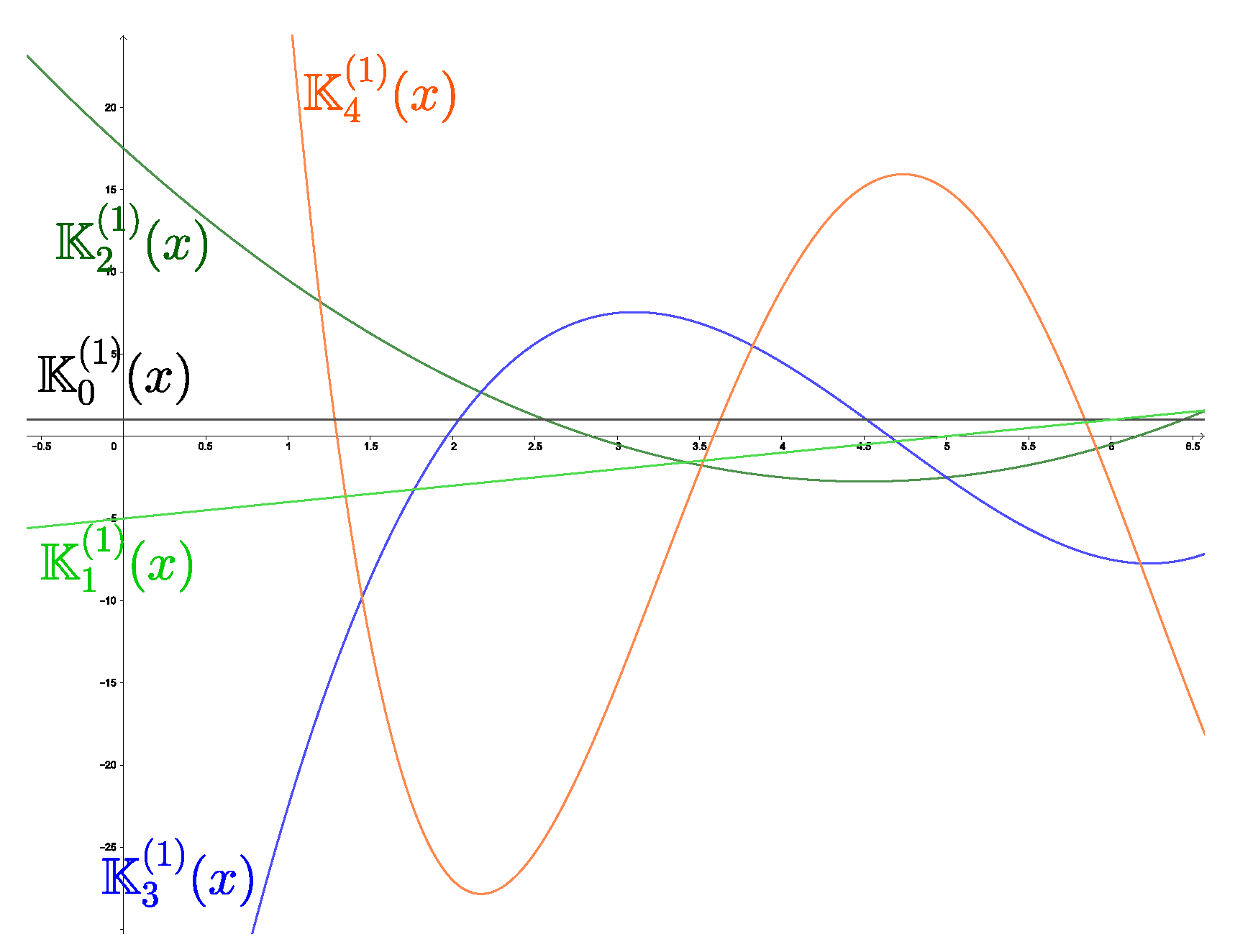
Figure 1 illustrates the Krawtchouk–Sobolev type polynomials for the values $N=10$, $p=1/2$, and with $j=1$. Observe in this case that the first ones coincide with the classical Krawtchouk polynomials in view of Proposition 2.

For the sake of a more compact writing of the forthcoming properties associated with such a family of polynomials, we put

$${\mathcal{C}}_{2,n}^{\left(j\right)}\left(x\right)=-\frac{{\mathcal{D}}_{1,n-1}^{\left(j\right)}\left(x\right)}{{\beta }_{n-1}^{p,N}},$$

$${\mathcal{D}}_{2,n}^{\left(j\right)}\left(x\right)={\mathcal{C}}_{1,n-1}^{\left(j\right)}\left(x\right)+{\mathcal{C}}_{2,n}^{\left(j\right)}\left(x\right)\left({\alpha }_{n-1}^{p,N}-x\right),$$

$${\mathcal{E}}_{1,n}^{\left(j\right)}\left(x\right)=x\nabla {\mathcal{C}}_{1,n}^{\left(j\right)}\left(x\right)+n{\mathcal{C}}_{1,n}^{\left(j\right)}(x-1)-\frac{\left(n-1\right)p\left(N-n+2\right){\mathcal{D}}_{1,n}^{\left(j\right)}(x-1)}{{\beta }_{n-1}^{p,N}},$$

$${\mathcal{F}}_{1,n}^{\left(j\right)}\left(x\right)=$$

$$\begin{array}{ccc}& & x\nabla {\mathcal{D}}_{1,n}^{\left(j\right)}\left(x\right)+np\left(N-n+1\right){\mathcal{C}}_{1,n}^{\left(j\right)}(x-1)\hfill \\ & & +\frac{\left(n-1\right)p\left(N-n+2\right)\left(x-{\alpha }_{n-1}^{p,N}\right){\mathcal{D}}_{1,n}^{\left(j\right)}(x-1)}{{\beta }_{n-1}^{p,N}}+\left(n-1\right){\mathcal{D}}_{1,n}^{\left(j\right)}(x-1),\hfill \end{array}$$

and

$${\mathcal{E}}_{2,n}^{\left(j\right)}\left(x\right)=-\frac{{\mathcal{F}}_{1,n-1}^{\left(j\right)}\left(x\right)}{{\beta }_{n-1}^{p,N}},$$

$${\mathcal{F}}_{2,n}^{\left(j\right)}\left(x\right)={\mathcal{E}}_{1,n-1}^{\left(j\right)}\left(x\right)+{\mathcal{E}}_{2,n}^{\left(j\right)}\left(x\right)\left({\alpha }_{n-1}^{p,N}-x\right).$$

We observe that the choice of the elements involved in the definition of the Krawtchouk–Sobolev type orthogonal polynomials is implicitly made, and will be omitted for simplicity. The properties of the sequence ${\{{\mathbb{K}}_n^{\left(j\right)}\left(x\right)\}}_{n\ge 0}$ determine analogous properties for this novel sequence of orthogonal Sobolev-type orthogonal polynomials.

Proposition 3.

Let ${\{{\mathbb{K}}_n^{\left(j\right)}\left(x\right)\}}_{n\ge 0}$ be the sequence of monic Krawtchouk–Sobolev orthogonal polynomials defined by (6). Then, the following statements hold.

1. 

Hypergeometric representation. Given positive integers $n\le N$ and j, one has

$${\mathbb{K}}_n^{\left(j\right)}\left(x\right)=p^{n-1}{\left(-N\right)}_{n-1}{h}_n^{\left(j\right)}\left(x\right){}_3{F}_2\left(\begin{array}{cc}-n,-x,f_n^{\left(j\right)}\left(x\right)& \\ -N,f_n^{\left(j\right)}\left(x\right)-1\end{array}|p^{-1}\right),$$

where

$$f_n^{\left(j\right)}\left(x\right)=\frac{np\left(N-n+1\right){\mathcal{C}}_{1,n}^{\left(j\right)}\left(x\right)}{{\mathcal{D}}_{1,n}^{\left(j\right)}\left(x\right)}-n+1,$$

and

$$h_n^{\left(j\right)}\left(x\right)=-\left(p\left(N-n+1\right){\mathcal{C}}_n^{\left(j\right)}\left(x\right)-{\mathcal{D}}_n^{\left(j\right)}\left(x\right)\right).$$

2. 

Structure relations.

$${\Theta }_n^{\left(j\right)}\left(x\right)\nabla {\mathbb{K}}_n^{\left(j\right)}\left(x\right)+{\Lambda }_n^{\left(j\right)}\left(x;2,1\right){\mathbb{K}}_n^{\left(j\right)}\left(x\right)={\Lambda }_n^{\left(j\right)}\left(x;1,1\right){\mathbb{K}}_{n-1}^{\left(j\right)}\left(x\right)$$

and

$${\Theta }_n^{\left(j\right)}\left(x\right)\nabla {\mathbb{K}}_{n-1}^{\left(j\right)}\left(x\right)+{\Lambda }_n^{\left(j\right)}\left(x;1,2\right){\mathbb{K}}_{n-1}^{\left(j\right)}\left(x\right)={\Lambda }_n^{\left(j\right)}\left(x;2,2\right){\mathbb{K}}_n^{\left(j\right)}\left(x\right),$$

where

$${\Theta }_n^{\left(j\right)}\left(x\right)=x\left|\begin{array}{cc}{\mathcal{C}}_{1,n}^{\left(j\right)}\left(x\right)& {\mathcal{C}}_{2,n}^{\left(j\right)}\left(x\right)\\ {\mathcal{D}}_{1,n}^{\left(j\right)}\left(x\right)& {\mathcal{D}}_{2,n}^{\left(j\right)}\left(x\right)\end{array}\right|,$$

and

$${\Lambda }_n^{\left(j\right)}\left(x;i,k\right)={\left(-1\right)}^k\left|\begin{array}{cc}{\mathcal{E}}_{k,n}^{\left(j\right)}\left(x\right)& {\mathcal{C}}_{i,n}^{\left(j\right)}\left(x\right)\\ {\mathcal{F}}_{k,n}^{\left(j\right)}\left(x\right)& {\mathcal{D}}_{i,n}^{\left(j\right)}\left(x\right)\end{array}\right|,i=1,2,k=1,2.$$

3. 

Second-order difference equations.

$${\mathcal{F}}_n^{\left(j\right)}\left(x\right){\nabla }^2{\mathbb{K}}_n^{\left(j\right)}\left(x\right)+{\mathcal{G}}_n^{\left(j\right)}\left(x\right)\nabla {\mathbb{K}}_n^{\left(j\right)}\left(x\right)+{\mathcal{H}}_n^{\left(j\right)}\left(x\right){\mathbb{K}}_n^{\left(j\right)}\left(x\right)=0,$$

and

$${\tilde{\mathcal{F}}}_n^{\left(j\right)}\left(x\right)\Delta \nabla {\mathbb{K}}_n^{\left(j\right)}\left(x\right)+{\tilde{\mathcal{G}}}_n^{\left(j\right)}\left(x\right)\Delta {\mathbb{K}}_n^{\left(j\right)}\left(x\right)+{\tilde{\mathcal{H}}}_n^{\left(j\right)}\left(x\right){\mathbb{K}}_n^{\left(j\right)}\left(x\right)=0,$$

where

$${\mathcal{F}}_n^{\left(j\right)}\left(x\right)={\Theta }_n^{\left(j\right)}\left(x\right){\Theta }_n^{\left(j\right)}\left(x-1\right),$$

$$\begin{array}{ccc}\hfill {\mathcal{G}}_n^{\left(j\right)}\left(x\right)& =& {\Theta }_n^{\left(j\right)}\left(x\right)(\nabla {\Theta }_n^{\left(j\right)}\left(x\right)+{\Lambda }_n^{\left(j\right)}\left(x-1;2,1\right)+{\Lambda }_n^{\left(j\right)}\left(x;1,2\right))\hfill \\ & & -\frac{\nabla {\Lambda }_n^{\left(j\right)}\left(x;1,1\right)({\Theta }_n^{\left(j\right)}\left(x\right)+{\Lambda }_n^{\left(j\right)}\left(x;1,2\right)){\Theta }_n^{\left(j\right)}\left(x\right)}{{\Lambda }_n^{\left(j\right)}\left(x;1,1\right)},\hfill \end{array}$$

$$\begin{array}{ccc}\hfill {\mathcal{H}}_n^{\left(j\right)}\left(x\right)& =& {\Theta }_n^{\left(j\right)}\left(x\right)\nabla {\Lambda }_n^{\left(j\right)}\left(x;2,1\right)+{\Lambda }_n^{\left(j\right)}\left(x;1,2\right){\Lambda }_n^{\left(j\right)}\left(x;2,1\right)\hfill \\ & & -\frac{\nabla {\Lambda }_n^{\left(j\right)}\left(x;1,1\right){\Lambda }_n^{\left(j\right)}\left(x;2,1\right)({\Theta }_n^{\left(j\right)}\left(x\right)+{\Lambda }_n^{\left(j\right)}\left(x;1,2\right))}{{\Lambda }_n^{\left(j\right)}\left(x;1,1\right)}\hfill \\ & & -{\Lambda }_n^{\left(j\right)}\left(x-1;1,1\right){\Lambda }_n^{\left(j\right)}\left(x;2,2\right),\hfill \end{array}$$

$${\tilde{\mathcal{F}}}_n^{\left(j\right)}\left(x\right)={\mathcal{F}}_n^{\left(j\right)}\left(x+1\right),and{\tilde{\mathcal{H}}}_n^{\left(j\right)}\left(x\right)={\mathcal{H}}_n^{\left(j\right)}\left(x+1\right),$$

and

$${\tilde{\mathcal{G}}}_n^{\left(j\right)}\left(x\right)={\mathcal{G}}_n^{\left(j\right)}\left(x+1\right)+{\tilde{\mathcal{H}}}_n^{\left(j\right)}\left(x\right).$$

4. 

The recurrence relation for the classical Krawtchouk monic orthogonal polynomials determines that, for the Krawtchouk–Sobolev type orthogonal polynomials, as follows:

$${\tilde{\Theta }}_n^{\left(j\right)}\left(x\right){\mathbb{K}}_{n+1}^{\left(j\right)}\left(x\right)={\Xi }_{1,n}^{\left(j\right)}\left(x\right){\mathbb{K}}_n^{\left(j\right)}\left(x\right)+{\Xi }_{2,n}^{\left(j\right)}\left(x\right){\mathbb{K}}_{n-1}^{\left(j\right)}\left(x\right),n\ge 0,$$

(10)

where

$${\tilde{\Theta }}_n^{\left(j\right)}\left(x\right)={\Theta }_n^{\left(j\right)}\left(x\right){\Lambda }_{n+1}^{\left(j\right)}\left(x;2,2\right),$$

$${\Xi }_{1,n}^{\left(j\right)}\left(x\right)={\Theta }_n^{\left(j\right)}\left(x\right){\Lambda }_{n+1}^{\left(j\right)}\left(x;1,2\right)-{\Theta }_{n+1}^{\left(j\right)}\left(x\right){\Lambda }_n^{\left(j\right)}\left(x;2,1\right),$$

and

$${\Xi }_{2,n}^{\left(j\right)}\left(x\right)={\Theta }_{n+1}^{\left(j\right)}\left(x\right){\Lambda }_n^{\left(j\right)}\left(x;1,1\right),$$

with initial conditions ${\mathbb{K}}_{-1}^{\left(j\right)}\left(x\right)=0$, and ${\mathbb{K}}_0^{\left(j\right)}\left(x\right)=1$.

In the remaining part of this Section, we complete the previous properties with the norm of the elements in ${\{{\mathbb{K}}_n^{\left(j\right)}\left(x\right)\}}_{n\ge 0}$, stated in Theorem 1. This result is derived from the Proposition 4, whose proof is a direct result of the following technical Lemma, together with (6).

Lemma 2.

For every $p,q\in \mathbb{P}$ one can apply the definition of the inner product to arrive at

$$\begin{array}{ccc}\hfill {〈{[x-N]}_{j+1}{\left[x\right]}_{j+1}p\left(x\right),q\left(x\right)〉}_{\lambda ,\mu }& =& {〈p\left(x\right),{[x-N]}_{j+1}{\left[x\right]}_{j+1}q\left(x\right)〉}_{\lambda ,\mu }\hfill \\ & =& 〈{[x-N]}_{j+1}{\left[x\right]}_{j+1}p\left(x\right),q\left(x\right)〉\hfill \\ & =& 〈p\left(x\right),{[x-N]}_{j+1}{\left[x\right]}_{j+1}q\left(x\right)〉.\hfill \end{array}$$

(11)

Proposition 4.

Let ${\{{\mathbb{K}}_n^{\left(j\right)}\left(x\right)\}}_{n\ge 0}$ be the sequence of monic Krawtchouk–Sobolev orthogonal polynomials defined by (6). Then, one has

$${\left[x\right]}_{j+1}{[x-N]}_{j+1}{\mathbb{K}}_n^{\left(j\right)}\left(x\right)={\Phi }_{1,n}^{\left(j\right)}\left(x\right)K_n^{p,N}\left(x\right)+{\Phi }_{2,n}^{\left(j\right)}\left(x\right)K_{n-1}^{p,N}\left(x\right),n\ge 0,$$

(12)

where

$${\Phi }_{1,n}^{\left(j\right)}\left(x\right)={\left[x\right]}_{j+1}{[x-N]}_{j+1}+{[x-N]}_{j+1}\sum _{k=0}^j{a}_{1,n}^{\left(k\right)}{\left[x\right]}_k+{\left[x\right]}_{j+1}\sum _{k=0}^j{a}_{2,n}^{\left(k\right)}{[x-N]}_k$$

(13)

and

$${\Phi }_{2,n}^{\left(j\right)}\left(x\right)={[x-N]}_{j+1}\sum _{k=0}^j{b}_{1,n}^{\left(k\right)}{\left[x\right]}_k+{\left[x\right]}_{j+1}\sum _{k=0}^j{b}_{2,n}^{\left(k\right)}{[x-N]}_k,$$

(14)

with $a_{i,n}^{\left(k\right)}$ and $b_{i,n}^{\left(k\right)}$ given in (7)–(8) and (9), respectively.

We denote $\left|\right|·{\left|\right|}_{\lambda ,\mu }$ the norm associated with the product ${〈·,·〉}_{\lambda ,\mu }$.

Theorem 1.

Let ${\{{\mathbb{K}}_n^{\left(j\right)}\left(x\right)\}}_{n\ge 0}$ be the sequence of monic Krawtchouk–Sobolev orthogonal polynomials defined by (6). Then, for every $\lambda ,\mu \in {\mathbb{R}}^{+}$, $j\in \mathbb{N}$, $0<p<1$ and $n\le N$ the norm of these orthogonal polynomials with respect to (5),

$$\left|\right|{\mathbb{K}}_n^{\left(j\right)}{\left|\right|}_{\lambda ,\mu }^2=\left|\right|K_n^{p,N}{\left|\right|}^2+(b_{1,n}^{\left(j\right)}+b_{2,n}^{\left(j\right)})\left|\right|K_{n-1}^{p,N}{\left|\right|}^2,$$

(15)

where $b_{1,n}^{\left(j\right)}$ and $b_{2,n}^{\left(j\right)}$ are determined in (9).

Proof. 

It is straightforward to check that

$$\left|\right|{\mathbb{K}}_n^{\left(j\right)}{\left|\right|}_{\lambda ,\mu }^2={〈{\mathbb{K}}_n^{\left(j\right)},{\left[x\right]}_{j+1}{[x-N]}_{j+1}{\pi }_{n-2j-2}\left(x\right)〉}_{\lambda ,\mu },$$

for every monic polynomial ${\pi }_{n-2j-2}$ of degree $n-2j-2$. In addition, from (11) we have

$$\begin{array}{ccc}\hfill {〈{\mathbb{K}}_n^{\left(j\right)},{\left[x\right]}_{j+1}{[x-N]}_{j+1}{\pi }_{n-2j-2}\left(x\right)〉}_{\lambda ,\mu }& =& {〈{\left[x\right]}_{j+1}{[x-N]}_{j+1}{\mathbb{K}}_n^{\left(j\right)},{\pi }_{n-2j-2}\left(x\right)〉}_{\lambda ,\mu }\hfill \\ & =& 〈{\left[x\right]}_{j+1}{[x-N]}_{j+1}{\mathbb{K}}_n^{\left(j\right)},{\pi }_{n-2j-2}\left(x\right)〉.\hfill \end{array}$$

Next we use the connection Formula (12). Taking into account that ${\Phi }_{1,n}^{\left(j\right)}\left(x\right)$ (see (13)) is a monic polynomial of degree exactly $2j+2$ and ${\Phi }_{2,n}^{\left(j\right)}\left(x\right)$ (see (14)) is a polynomial of degree exactly $2j+1$ with the leading coefficient $b_{1,n}^{\left(j\right)}+b_{2,n}^{\left(j\right)}$ we deduce

$$\begin{array}{ccc}\hfill \left|\right|{\mathbb{K}}_n^{\left(j\right)}{\left|\right|}_{\lambda ,\mu }^2& =& 〈{\Phi }_{1,n}^{\left(j\right)}\left(x\right)K_n^{p,N}\left(x\right),{\pi }_{n-2j-2}\left(x\right)〉+\hfill \\ & & +〈{\Phi }_{2,n}^{\left(j\right)}\left(x\right)K_{n-1}^{p,N}\left(x\right),{\pi }_{n-2j-2}\left(x\right)〉,\hfill \\ & =& 〈K_n^{p,N}\left(x\right),x^n〉+(b_{1,n}^{\left(j\right)}+b_{2,n}^{\left(j\right)})〈K_{n-1}^{p,N}\left(x\right),x^{n-1}〉,\hfill \end{array}$$

which leads to (15).    □

3. Weighted Krawtchouk–Sobolev Type Polynomials

This section is devoted to define the so-called weighted Krawtchouk–Sobolev type polynomials, and describe their main properties, which will be used in Section 5 in an application to watermarking schemes. The knowledge of the norm obtained in Theorem 1 is of great importance in order to define such weighted Krawtchouk–Sobolev type polynomials. It is worth remarking that, despite their name, the elements of the sequence of weighted Krawtchouk–Sobolev type polynomials are no longer polynomials. We have maintained this and other denominations to maintain the one used in applications such as that of Section 5. We refer to [22] for more information in this concern.

As in the previous sections, we fix the parameters defining the norm of a Krawtchouk–Sobolev sequence of monic orthogonal polynomials.

Definition 4.

Let ${\{{\mathbb{K}}_n^{\left(j\right)}\left(x\right)\}}_{n\ge 0}$ be the sequence of monic Krawtchouk–Sobolev orthogonal polynomials defined by (6) and let (15) be the norm of such polynomials. The weighted Krawtchouk–Sobolev type polynomial ${\overline{\mathbb{K}}}_n^{\left(j\right)}\left(x\right)$ is defined by

$${\overline{\mathbb{K}}}_n^{\left(j\right)}\left(x\right)={\mathbb{K}}_n^{\left(j\right)}\left(x\right)\sqrt{\frac{\rho \left(x\right)}{\left|\right|{\mathbb{K}}_n^{\left(j\right)}{\left|\right|}_{\lambda ,\mu }^2}},$$

(16)

for every $n\ge 0$.

In the next result, we obtain the asymptotic behavior as $\lambda$ and $\mu$ approach zero, which leads to the asymptotic behavior of the matrix of orthogonal direct moments, as defined in Section 5.

Lemma 3.

Let ${\{{\overline{\mathbb{K}}}_n^{\left(j\right)}\left(x\right)\}}_{n\ge 0}$ be the sequence of weighted Krawtchouk–Sobolev type polynomials defined by (16). Then, it holds that

$$\underset{(\lambda ,\mu )\to (0,0)}{lim}\sum _{x=0}^N{\overline{\mathbb{K}}}_m^{\left(j\right)}\left(x\right){\overline{\mathbb{K}}}_n^{\left(j\right)}\left(x\right)={\delta }_{m,n}.$$

Here, ${\delta }_{m,n}$ stands for the Kronecker delta.

Proof. 

From the definition of the Krawtchouk–Sobolev type orthogonal polynomials in (5), we then observe that

$$\sum _{x=0}^N{\mathbb{K}}_m^{\left(j\right)}\left(x\right){\mathbb{K}}_n^{\left(j\right)}\left(x\right)\rho \left(x\right)+\lambda {\Delta }^j{\mathbb{K}}_m^{\left(j\right)}\left(0\right){\Delta }^j{\mathbb{K}}_n^{\left(j\right)}\left(0\right)+\mu {\Delta }^j{\mathbb{K}}_m^{\left(j\right)}\left(N\right){\Delta }^j{\mathbb{K}}_n^{\left(j\right)}\left(N\right)$$

$$=\left|\right|{\mathbb{K}}_n^{\left(j\right)}{\left|\right|}_{\lambda ,\mu }^2{\delta }_{m,n}.$$

From the previous equality, one can conclude that

$$\sum _{x=0}^N{\mathbb{K}}_m^{\left(j\right)}\left(x\right)\sqrt{\frac{\rho \left(x\right)}{\left|\right|{\mathbb{K}}_n^{\left(j\right)}{\left|\right|}_{\lambda ,\mu }^2}}{\mathbb{K}}_n^{\left(j\right)}\left(x\right)\sqrt{\frac{\rho \left(x\right)}{\left|\right|{\mathbb{K}}_n^{\left(j\right)}{\left|\right|}_{\lambda ,\mu }^2}}$$

$$+\frac{1}{\left|\right|{\mathbb{K}}_n^{\left(j\right)}{\left|\right|}_{\lambda ,\mu }^2}\left[\lambda {\Delta }^j{\mathbb{K}}_m^{\left(j\right)}\left(0\right){\Delta }^j{\mathbb{K}}_n^{\left(j\right)}\left(0\right)+\mu {\Delta }^j{\mathbb{K}}_m^{\left(j\right)}\left(N\right){\Delta }^j{\mathbb{K}}_n^{\left(j\right)}\left(N\right)\right]={\delta }_{m,n}.$$

Therefore,

$$\underset{(\lambda ,\mu )\to (0,0)}{lim}\sum _{x=0}^N{\mathbb{K}}_m^{\left(j\right)}\left(x\right)\sqrt{\frac{\rho \left(x\right)}{\left|\right|{\mathbb{K}}_n^{\left(j\right)}{\left|\right|}_{\lambda ,\mu }^2}}{\mathbb{K}}_n^{\left(j\right)}\left(x\right)\sqrt{\frac{\rho \left(x\right)}{\left|\right|{\mathbb{K}}_n^{\left(j\right)}{\left|\right|}_{\lambda ,\mu }^2}}={\delta }_{m,n}.$$

   □

The following recurrence relation holds for the sequence of weighted Krawtchouk–Sobolev type polynomials.

Proposition 5.

Let ${\{{\overline{\mathbb{K}}}_n^{\left(j\right)}\left(x\right)\}}_{n\ge 0}$ be the sequence of weighted Krawtchouk–Sobolev type polynomials defined in (16). Then, the following recurrence relation holds:

$${\overline{\mathbb{K}}}_{n+1}^{\left(j\right)}\left(x\right)={\Psi }_{1,n}^{\left(j\right)}\left(x\right){\overline{\mathbb{K}}}_n^{\left(j\right)}\left(x\right)+{\Psi }_{2,n}^{\left(j\right)}\left(x\right){\overline{\mathbb{K}}}_{n-1}^{\left(j\right)}\left(x\right),n\ge 0,$$

where

$${\Psi }_{1,n}^{\left(j\right)}\left(x\right)=\frac{\left|\right|{\mathbb{K}}_n^{\left(j\right)}{\left|\right|}_{\lambda ,\mu }}{\left|\right|{\mathbb{K}}_{n+1}^{\left(j\right)}{\left|\right|}_{\lambda ,\mu }}\frac{{\Xi }_{1,n}^{\left(j\right)}\left(x\right)}{{\tilde{\Theta }}_n^{\left(j\right)}\left(x\right)}and{\Psi }_{2,n}^{\left(j\right)}\left(x\right)=\frac{\left|\right|{\mathbb{K}}_{n-1}^{\left(j\right)}{\left|\right|}_{\lambda ,\mu }}{\left|\right|{\mathbb{K}}_{n+1}^{\left(j\right)}{\left|\right|}_{\lambda ,\mu }}\frac{{\Xi }_{2,n}^{\left(j\right)}\left(x\right)}{{\tilde{\Theta }}_n^{\left(j\right)}\left(x\right)}.$$

Proof. 

A direct application of (10) yields

$${\mathbb{K}}_{n+1}^{\left(j\right)}\left(x\right)=\frac{{\Xi }_{1,n}^{\left(j\right)}\left(x\right)}{{\tilde{\Theta }}_n^{\left(j\right)}\left(x\right)}{\mathbb{K}}_n^{\left(j\right)}\left(x\right)+\frac{{\Xi }_{2,n}^{\left(j\right)}\left(x\right)}{{\tilde{\Theta }}_n^{\left(j\right)}}{\mathbb{K}}_{n-1}^{\left(j\right)}\left(x\right),n\ge 0.$$

The previous equation is equivalent to

$$\left|\right|{\mathbb{K}}_{n+1}^{\left(j\right)}{\left|\right|}_{\lambda ,\mu }{\mathbb{K}}_{n+1}^{\left(j\right)}\left(x\right)\sqrt{\frac{\rho \left(x\right)}{\left|\right|{\mathbb{K}}_{n+1}^{\left(j\right)}{\left|\right|}_{\lambda ,\mu }^2}}=$$

$$\frac{\left|\right|{\mathbb{K}}_n^{\left(j\right)}{\left|\right|}_{\lambda ,\mu }{\Xi }_{1,n}^{\left(j\right)}\left(x\right)}{{\tilde{\Theta }}_n^{\left(j\right)}\left(x\right)}{\mathbb{K}}_n^{\left(j\right)}\left(x\right)\sqrt{\frac{\rho \left(x\right)}{\left|\right|{\mathbb{K}}_n^{\left(j\right)}{\left|\right|}_{\lambda ,\mu }^2}}+\frac{\left|\right|{\mathbb{K}}_{n-1}^{\left(j\right)}{\left|\right|}_{\lambda ,\mu }^2{\Xi }_{2,n}^{\left(j\right)}\left(x\right)}{{\tilde{\Theta }}_n^{\left(j\right)}}{\mathbb{K}}_{n-1}^{\left(j\right)}\left(x\right)\sqrt{\frac{\rho \left(x\right)}{\left|\right|{\mathbb{K}}_{n-1}^{\left(j\right)}{\left|\right|}_{\lambda ,\mu }^2}},$$

and the result follows from here.    □

4. Krawtchouk–Sobolev Type Orthogonal Moments

In this section, we briefly describe the mathematical statements to be considered in the application for a watermarking scheme. For this reason, the notation stated in this section will be maintained in the last section of applications.

Assume one considers an image, the cover image, stored in matrix $\mathcal{C}$. Such a matrix is divided into matrices of size $N\times N$ bytes. The $k$-th image block of $\mathcal{C}$ is denoted by ${\mathcal{C}}^{(k,N)}$. Let us write

$${\mathcal{C}}^{(k,N)}=\left(\begin{array}{ccc}{\mathcal{C}}_{0,0}^{(k,N)}& \cdots & {\mathcal{C}}_{0,N-1}^{(k,N)}\\ ⋮& \ddots & ⋮\\ {\mathcal{C}}_{N-1,0}^{(k,N)}& \cdots & {\mathcal{C}}_{N-1,N-1}^{(k,N)}\end{array}\right).$$

Definition 5.

Let ${\mathcal{C}}^{(k,N)}$ be the $k$-th image block of a cover image $\mathcal{C}$. We define its matrix of orthogonal direct moments by

$$\mathcal{M}=\mathcal{A}{\mathcal{C}}^{(k,N)}{\mathcal{A}}^t,$$

(17)

where

$$\mathcal{A}=\left(\begin{array}{ccc}{\overline{\mathbb{K}}}_0^{\left(j\right)}\left(0\right)& \cdots & {\overline{\mathbb{K}}}_{N-1}^{\left(j\right)}\left(0\right)\\ ⋮& \ddots & ⋮\\ {\overline{\mathbb{K}}}_0^{\left(j\right)}(N-1)& \cdots & {\overline{\mathbb{K}}}_{N-1}^{\left(j\right)}(N-1)\end{array}\right),$$

(18)

for some fixed j.

The purpose of a steganographic image, created from a cover image, relies on the fact that the steganographic image hides some data within it, while maintaining a similar shape as that of the cover image, hiding secret data in it. The results obtained in Section 3, in particular Lemma 3, guarantees that ${\mathcal{A}}^t\mathcal{A}\approxeq \mathcal{I}$, where $\mathcal{I}$ denote the identity matrix.

The previous fact motivates the following transformation associated to $\mathcal{M}$.

Definition 6.

Let $\mathcal{M}$ be the matrix of orthogonal direct moments. The matrix of orthogonal inverse moments is given by

$${\mathcal{W}}^{(k,N)}={\mathcal{A}}^t\mathcal{M}\mathcal{A}.$$

(19)

According to Lemma 3 and (17), one has that

$${\mathcal{W}}^{(k,N)}={\mathcal{A}}^t\mathcal{M}\mathcal{A}={\mathcal{A}}^t\mathcal{A}{\mathcal{C}}^{(k,N)}{\mathcal{A}}^t\mathcal{A}$$

and therefore, one concludes

$$\underset{(\lambda ,\mu )\to (0,0)}{lim}{\mathcal{W}}^{(k,N)}={\mathcal{C}}^{(k,N)}.$$

Therefore, one can choose $\lambda ,\mu$ such that the watermarked image remains as close as needed to the cover image.

5. Application: Watermarking Scheme

In this section a watermarking scheme is presented as an application of the Krawtchouk–Sobolev type orthogonal moments. The embedding algorithm obtaining a watermarked image $\mathcal{W}$ from a cover image $\mathcal{C}$ is deduced following the procedure explained in the previous section. The present work concludes with the experimental analysis of the proposed scheme.

5.1. Arnold Transform

The Arnold transform is an invertible method that can be used for pixel scrambling. This important transform has been widely used in various watermarking schemes proposed by several authors. Arnold transform can be used in order to eliminate the high correlation of pixels, see [23]:

$$\left[\begin{array}{c}\widehat{x}\\ \widehat{y}\end{array}\right]=\left[\begin{array}{cc}1& p\\ q& pq+1\end{array}\right]\left[\begin{array}{c}x\\ y\end{array}\right]\left(modN\right).$$

(20)

The watermark is scrambled from $\omega$ into $\widehat{\omega }$. Here, $(x,y)$ y $(\widehat{x},\widehat{y})$ represent the pixels of $\omega$ and $\widehat{\omega }$, respectively. In particular, we take $p=1$ and $q=\eta$, being $\eta$ the control parameter, which is used as a private key during the watermark embedding and extraction processes.

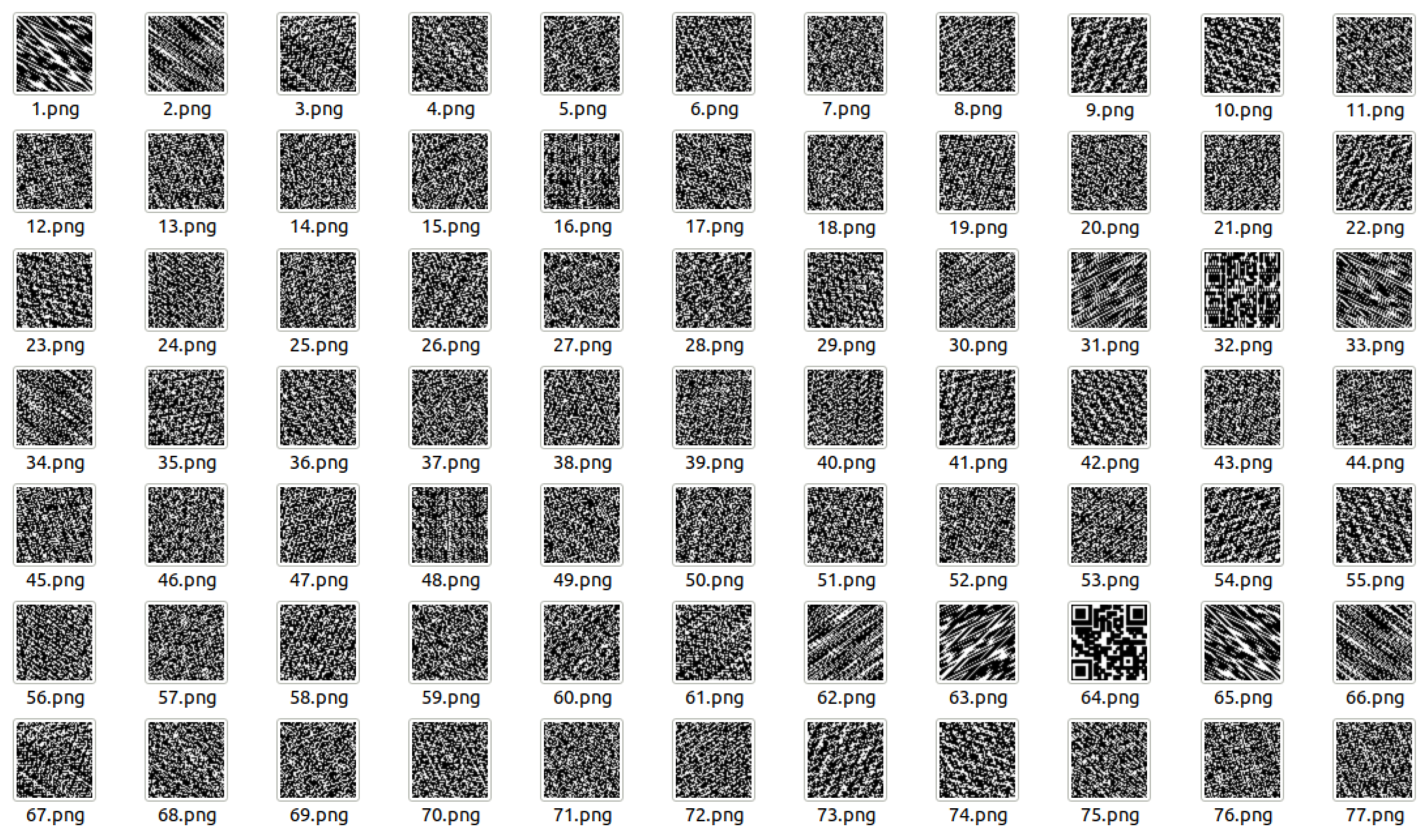
The watermark that will be used in this contribution is that of Figure 2:

Thus, considering Figure 3, it is deduced that the control parameter $\eta$ should satisfy that $\eta \in [1,63]$, since for $\eta =64$ the watermark is recovered in the process of applying the Arnold transform.

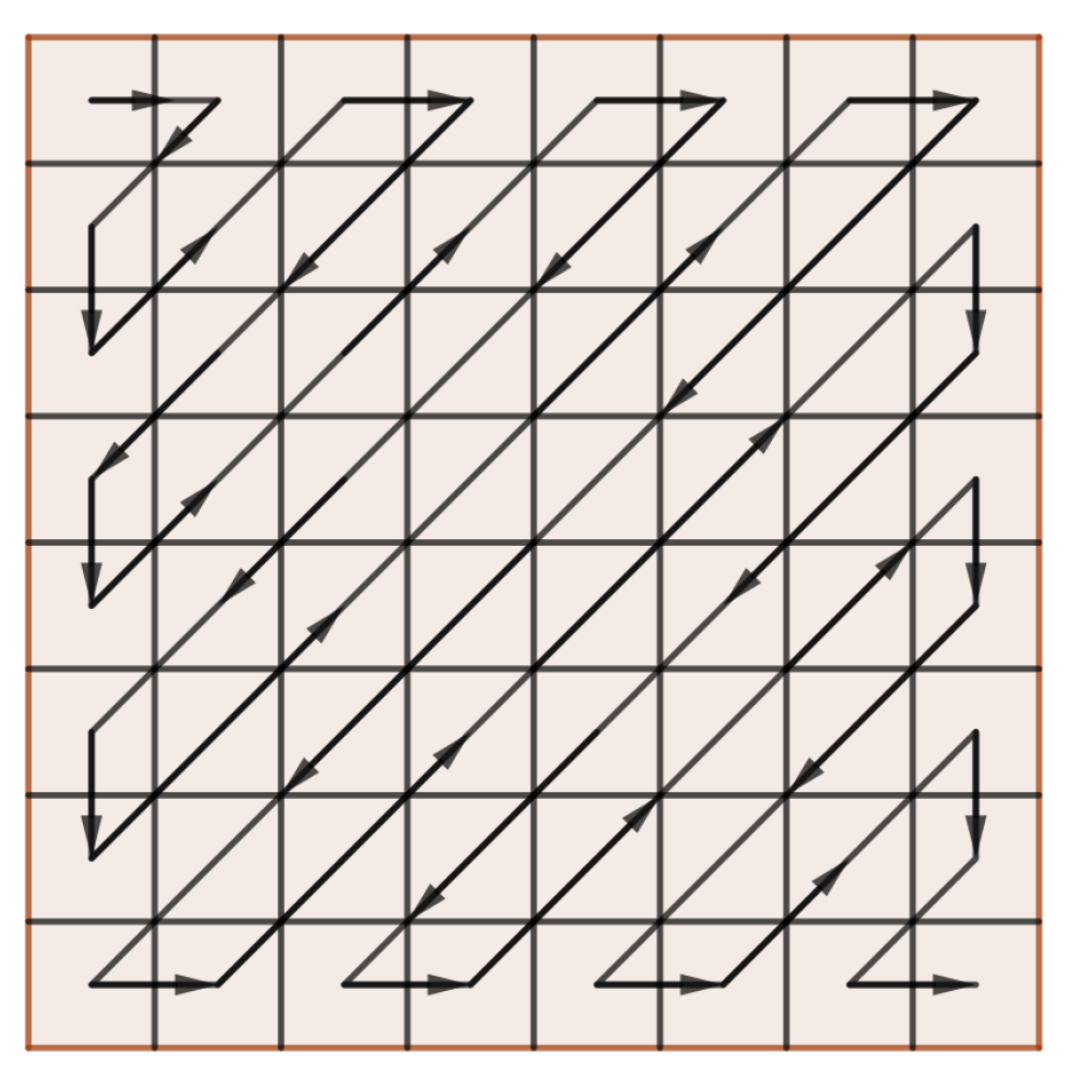
5.2. Zigzag Scan

Following the notation considered in [22], we write $\mathcal{Z}(·)$ for the operator transforming a $8\times 8$ matrix into a vector of length 64 after the ordering given to the elements of the matrix determined by the zigzag scan (see Figure 4). The inverse operator ${\mathcal{Z}}^{-1}(·)$ sends a vector of length 64 to a matrix of order 8 with ${\mathcal{Z}}^{-1}\circ \mathcal{Z}$ being the identity sending a matrix of order 8 to itself, and $\mathcal{Z}\circ {\mathcal{Z}}^{-1}$ is the operator sending a vector of length 64 to itself. The symbol ∘ stands for the composition operator.

5.3. Dither Modulation

Dither Modulation (DM) is a special form of quantization index molulation that is applied in an image watermarking system in order to assign one bit to each transformation coefficient. In case of a uniform scalar quantization, see [24,25], the watermarked signal is given by

$$y_n={\mathcal{Q}}_{\Delta }\left(x_n+d_m\right)-d_m,m\in \{0,1\},n=1,\dots ,L,$$

where $\Delta$ denotes the quantization step size that controls the embedding strength of the watermark bit. In addition, ${\mathcal{Q}}_{\Delta }(·)$ is defined as follows

$${\mathcal{Q}}_{\Delta }\left(\alpha \right)=\Delta \times round\left(\frac{\alpha }{\Delta }\right),$$

where round $(·)$ denotes the round function to the nearest integer. Moreover, $x_n$ represents the signal, $d_m$ the dither value, m the message, and L denotes the number of elements of m. In an uncoded case of binary dither modulation with an embedding rate one, the quantizers are constructed with the constraint

$$d_1=\left\{\begin{array}{cc}{\displaystyle d_0-\frac{\Delta }{2},}\hfill & d_0\ge 0,\hfill \\ \\ {\displaystyle d_0+\frac{\Delta }{2},}\hfill & d_0<0,\hfill \end{array}\right.$$

which complies with the following

$$-\frac{\Delta }{2}\le d_0\le \frac{\Delta }{2}.$$

In particular, in this contribution we have taken $d_0=-\Delta /4$.

For this embedding method, the received signal ${\widehat{y}}_n$ is a possibly corrupted version of $y_n$, which is re-quantized with the family of quantizers used during embedding to determine the bit of the embedded message

$$\widehat{m}={\mathrm{argmin}}_{m\in \{0,1\}}|{\mathcal{Q}}_{\Delta }\left({\widehat{y}}_n+d_m\right)-{\widehat{y}}_n|,$$

where argmin returns the indices of the minimum values along an axis.

5.4. Embedding and Extraction Watermark Algorithm

First, the embedding watermark algorithm scrambles the watermark by the Arnold transform (20) for a control parameter $\eta$, with $1\le \eta \le 63$, see Figure 3, and then it is organized into a binary sequence $\{{\widehat{\omega }}_i\}$, $i=1,\dots ,64\times 64$. Next, this scheme splits the cover image $\mathcal{C}$ into non-overlapping blocks ${\mathcal{C}}^{(k,8)}$ of size $8\times 8$, where the number of blocks coincide with the number of watermark bits. On the other hand, it applies the direct moments (17) to each block of $8\times 8$. Next, the zigzag scan is applied to the resultant coefficients block, see Figure 4, with the purpose to align frequency coefficients in ascending order. Then, it selects a coefficient of (17), in this case, the coefficient number is 28. Thus, the secret bits are embedded in the selected coefficient by applying the Dither Modulation (DM). Finally, the inverse moment transform (19) is applied in order to reconstruct the image, obtaining the watermarked image ${\mathcal{W}}^{(k,8)}$.

Algorithm 1 describes the procedure explained in Section 4 at the time of watermarking a cover image $\mathcal{C}$.

Algorithm 1 Embedding Algorithm

1: Input: Cover image $\mathcal{C}$, watermark $\{{\omega }_i\in \{0,1\}:i=1,2,\dots \}$ 2: Output: Watermarked image $\mathcal{W}$ 3: $\{{\widehat{\omega }}_i\}\leftarrow$ scrambled watermark by the Arnold transform (20). 4: Divide $\mathcal{C}$ into non-overlapping blocks of $8\times 8$ bytes 5: for each${\mathcal{C}}^{(k,8)}\in \mathcal{C}$do 6:    $\mathcal{M}\leftarrow \mathcal{A}{\mathcal{C}}^{(k,N)}{\mathcal{A}}^t$: according to (17) 7:    ${\nu }^k\leftarrow \mathcal{Z}\left(\mathcal{M}\right)$: Apply the zigzag scan 8:    ${\overline{\nu }}_{28}^k\leftarrow {\nu }_{28}^k$ watermark bit ${\widehat{\omega }}_k$ is embedded in the selected coefficient ${\nu }_{28}^k$ by using Dither Modulation. 9:    $\overline{\mathcal{M}}\leftarrow {\mathcal{Z}}^{-1}\left({\overline{\nu }}^k\right)$ 10:    ${\mathcal{W}}^{(k,N)}\leftarrow {\mathcal{A}}^t\mathcal{M}\mathcal{A}$: According to (19) 11: end for 12: return$\mathcal{W}$

The extraction process is similar to the embedding process detailed above.

5.5. Experimental Analysis

In this section we describe the experimental results of the proposed scheme. Changes in the cover image pixel values appear due to the cover image being altered to embed the secret data. The changes made on the image need to be analyzed since it directly affect the imperceptibility of the output stego image.

For the experimental analysis several color images of size ($512\times 512$) were used from two different datasets: a first image dataset of 1500 RGB-BMP images, transformed from Caltech birds’ dataset in JPEGC format [26] (Dataset I) and a second image dataset of 1500 RGB-BMP images, transformed from NRC dataset in TIFF format [26] (Dataset II). Since the cover images are of size $512\times 512$ and the watermark is $64\times 64$ bits, see Figure 2, then the watermark bits are distributed in each block throughout the original image. The algorithm proposed in the present work is implemented in Python 3.8.10.

The results of the experimental analysis are displayed in the following figures in which the PSNR values of the watermarked images corresponding to each of the two datasets are considered. More precisely, we show the values of PSNR of Krawtchouk polynomials (K) and the proposed Krawtchouk–Sobolev type polynomials (KSX), where $X\in \{1,2,3\}$ determines the value of j in the definition of such polynomials. In addition, a comparison of the proposed method for Krawtchouk moments (KMs, $p=0.5$) with respect to the method proposed for Krawtchouk–Sobolev type orthogonal moments (KS1Ms with $p=0.5$, $\lambda =\mu ={10}^{-7}$, KS2Ms with $p=0.5$, $\lambda =\mu ={10}^{-10}$, and KS3Ms with $p=0.5$, $\lambda =\mu ={10}^{-11}$) is included in this section.

Moreover, a comparison of the proposed moments with respect to the moments proposed by Yamni et al., Fractional Moments of Charlier (FrCMs) [27] and Yamni et al., Fractional Moments of Charlier–Meixner (FrCMMs) [28] is included in this section. The following attacks to measure robustness were applied: Cropping noise, Gaussian noise, Salt & Pepper noise, and Median filter noise.

In order to make a fair comparison with the FrCMs and FrCMMs moments in relation to KMs, KS1Ms, KS2Ms, and KS3Ms, the quantization steps $\Delta =30$ and $\Delta =50$ were chosen for the experiments, maintaining a PSNR value close to 50 dB. For the moments KMs, KS1Ms, KS2Ms, and KS3Ms, $\Delta =50$ was used. The performance of the proposed approach has been studied using the following of statistical measures.

5.6. Imperceptibility Test

The measure of the quality of the watermarked image is made in terms of PSNR (Peak Signal to Noise Ratio) of different datasets. PSNR is widespread and a top notch metric is used in order to measure the quality of the watermarked image. It analyzes the mean squared error value, comparing the cover and the stego image [29].

PSNR is defined by

$$\mathrm{PSNR}=10{log}_{10}\left({\displaystyle \frac{{\displaystyle {\Xi }^2}}{{\displaystyle \mathrm{MSE}}}}\right),$$

with

$$\mathrm{MSE}={\left(N^2\rho \right)}^{-1}\sum _{\mathbf{fl}\in \Gamma }{∥\mathcal{C}\left(\mathbf{fl}\right)-\mathcal{W}\left(\mathbf{fl}\right)∥}^2.$$

$\mathcal{C}$ and $\mathcal{W}$ represent the cover image and the stego image, respectively, of size $N^2\rho$, with $\mathcal{C},\mathcal{W}\in \{0,1,\cdots ,\Xi \}$, and $\Xi =\max \left(\max \right(\mathcal{C}),\max (\mathcal{W}\left)\right)$.

The index set $\mathbf{fl}=({\ell }_1,{\ell }_2,{\ell }_3)$ sums over the set

$$\Gamma =\{1,\cdots ,m\}\times \{1,\cdots ,n\}\times \{1,\cdots ,\rho \},$$

where $\rho =1$ for gray scale images and $\rho =3$ for 24-bit color images.

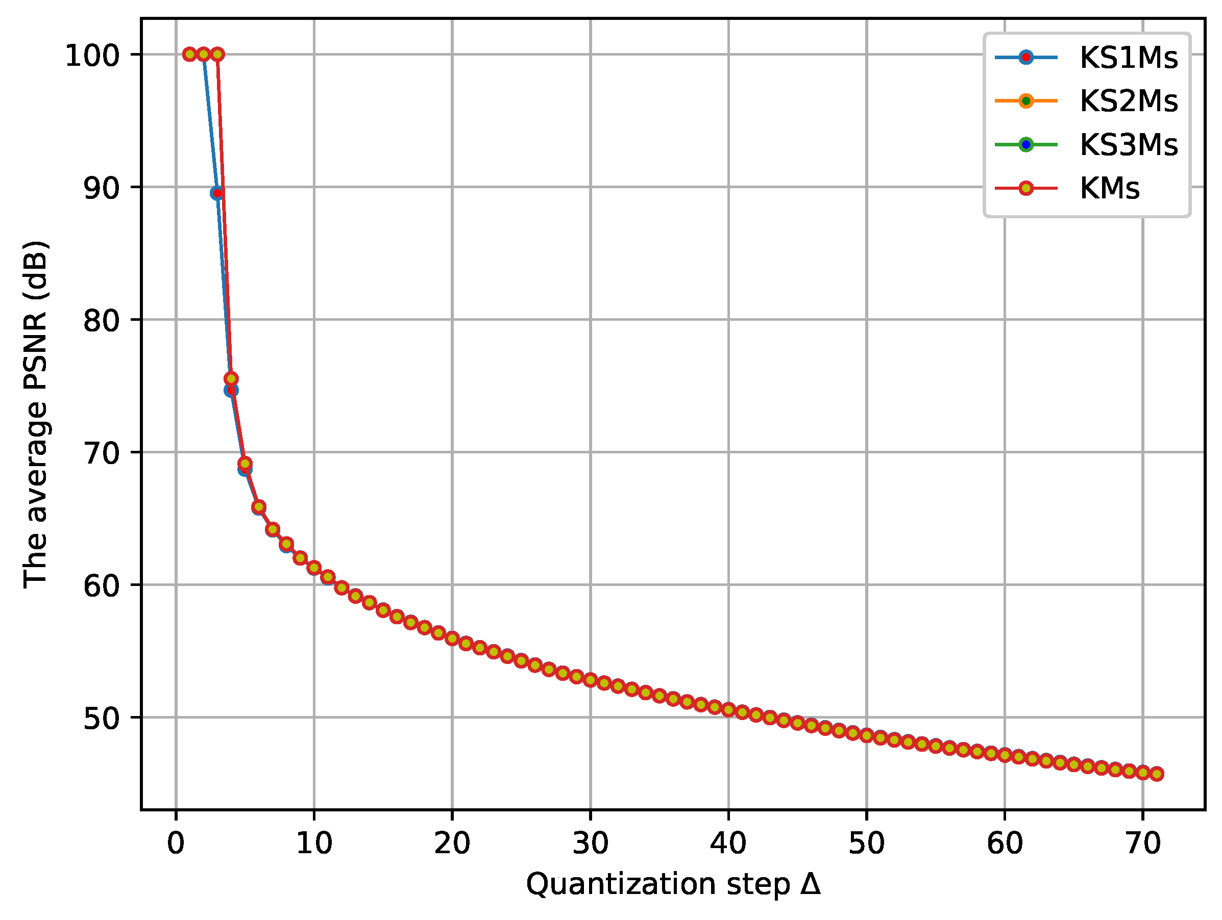
In the first experiment, we use the PSNR as a measure to evaluate the level of imperceptibility and distortion as well as to measure the difference between cover and watermarked images. The experimental results showed that the proposed moments produced good quality watermarked images with good PSNR values, see Figure 5, which is in correspondence with the heuristic values of PSNR. On the other hand, in Figure 5, it is possible to observe that as the quantization step increases, the average PSNR decreases. Moreover, this experiment showed that for the two datasets, the results of imperceptibility corresponding to the KMs, KS1Ms, KS2Ms, and KS3Ms are similar. This is interesting, since a priori no differences are shown. However, the next study demonstrates the strength of KS1Ms, KS2Ms, and KS3Ms in relation to KMs.

5.7. Robustness Test

The robustness is measured as the bit error rate (BER) corresponding to incorrectly formed binary values of the watermark image. The BER value is calculated by using the equation

$$\mathrm{BER}=\frac{1}{L}\sum _{n=0}^{L-1}\left\{\begin{array}{cc}1,\hfill & \overline{\omega }\left(n\right)\ne \omega \left(n\right),\hfill \\ 0,\hfill & \overline{\omega }\left(n\right)=\omega \left(n\right),\hfill \end{array}\right.$$

where $\omega \left(n\right)$ and $\overline{\omega }\left(n\right)$ are binary bits (0 or 1) of the original watermark and the extracted watermark. Moreover, L is the number of bits of the watermark.

In order to evaluate the robustness, the following attacks were applied: Cropping noise, Gaussian noise, Salt and Pepper noise, and Median filter noise. Their parameters appear in

Table 1. Information of the applied attacks.

Attacks	Parameters
Cropping noise	5%, 10%, 12%, 15%, 17%, 20%, 23%, 25%, 27%, 30%, 33%, 35%, 37%, 40%.
Gaussian noise	Percent noise: 0.01, 0.02, 0.03, 0.04, 0.05, 0.06, 0.07, 0.08
Salt and Pepper noise	Density: 0.01, 0.02, 0.03, 0.04, 0.05, 0.06, 0.07, 0.08
Median filter noise	Kernel size: 2 × 2, 4 × 4, 6 × 6, 8 × 7, 10 × 10, 12 × 12, 14 × 14, 16 × 16, 18 × 18, 20 × 20

.

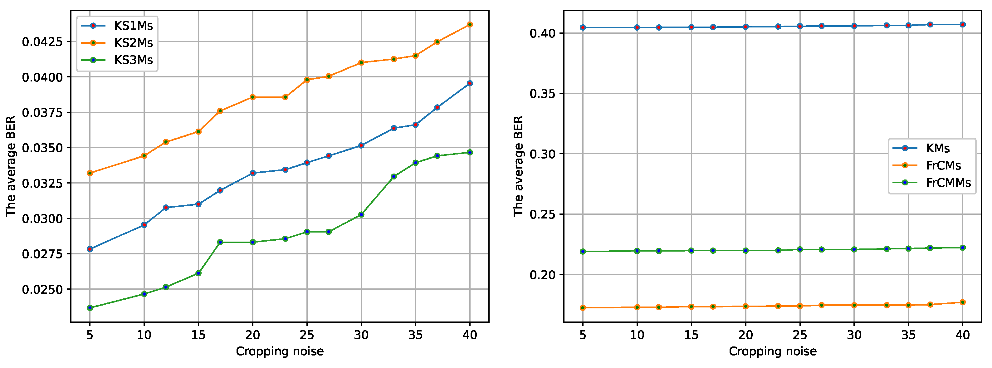
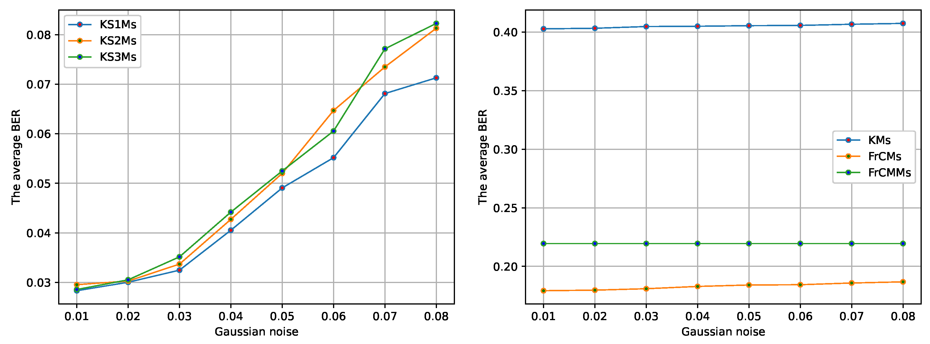
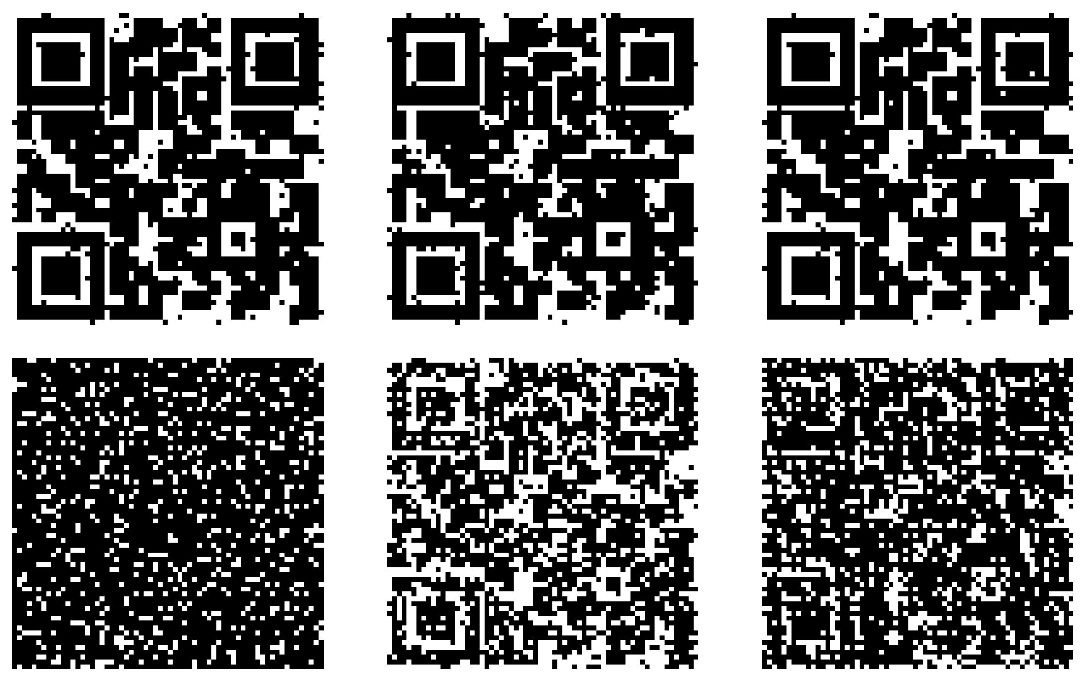
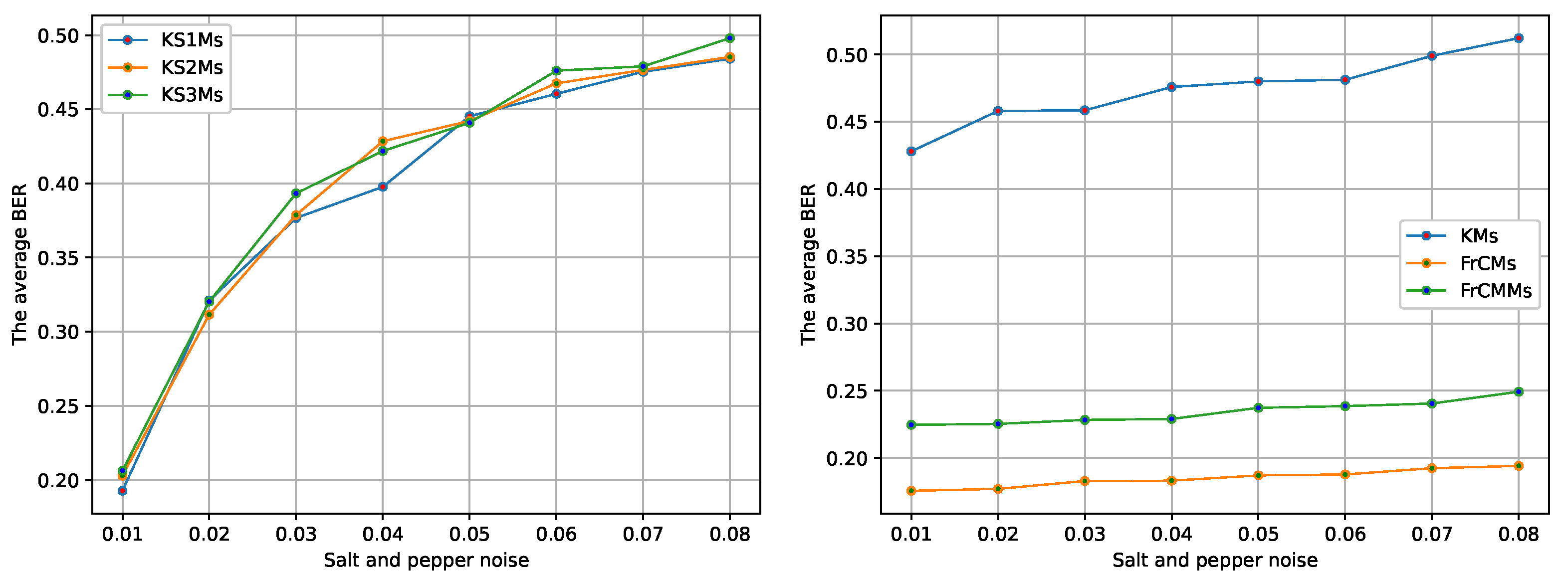
In this experiment, it is shown in the results displayed in Figure 6, Figure 7 and Figure 8, that robustness of the watermarking scheme based on KS1Ms, KS2Ms, and KS3Ms is much higher than that of the schemes based on KMs, KMs, and FrCMs. Moreover, the KMs do not resist well to the attacks performed in this contribution since the BER values are higher, see Figure 9Figure 10. On the other hand, for Salt & Pepper noise displayed in Figure 11, the moments FrCMs and FrCMMs seem to be more robust with respect to the schemes based on KS1Ms, KS2Ms, KS3Ms, and KMs.

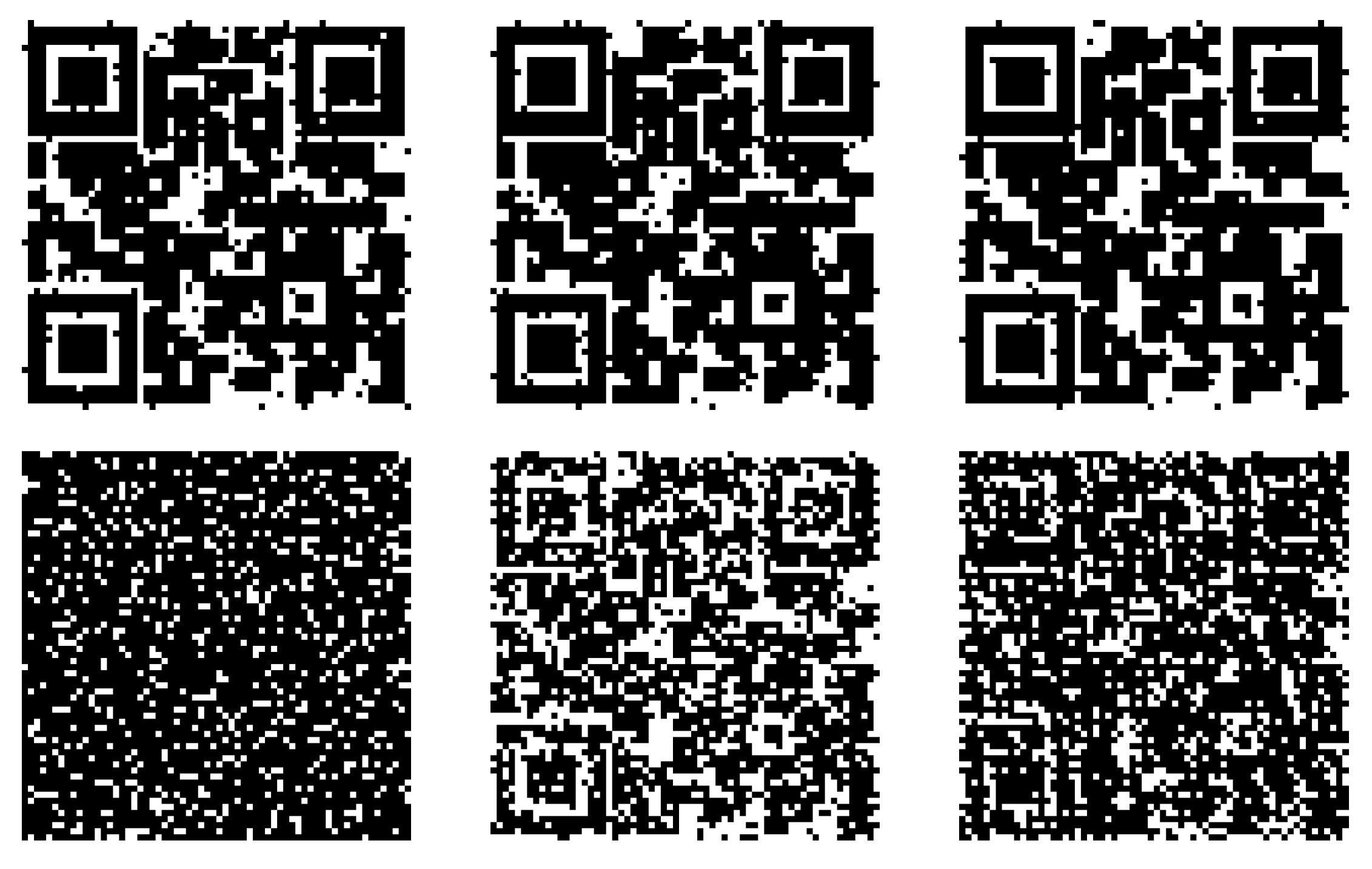
The BER values are close to zero, obtained after applying the attacks (Cropping noise and Gaussian noise), corresponding to KS1Ms, KS2Ms, and KS3Ms. This means that the extracted watermarks are recognizable and very similar to the original watermarks, see Figure 9 and Figure 10.

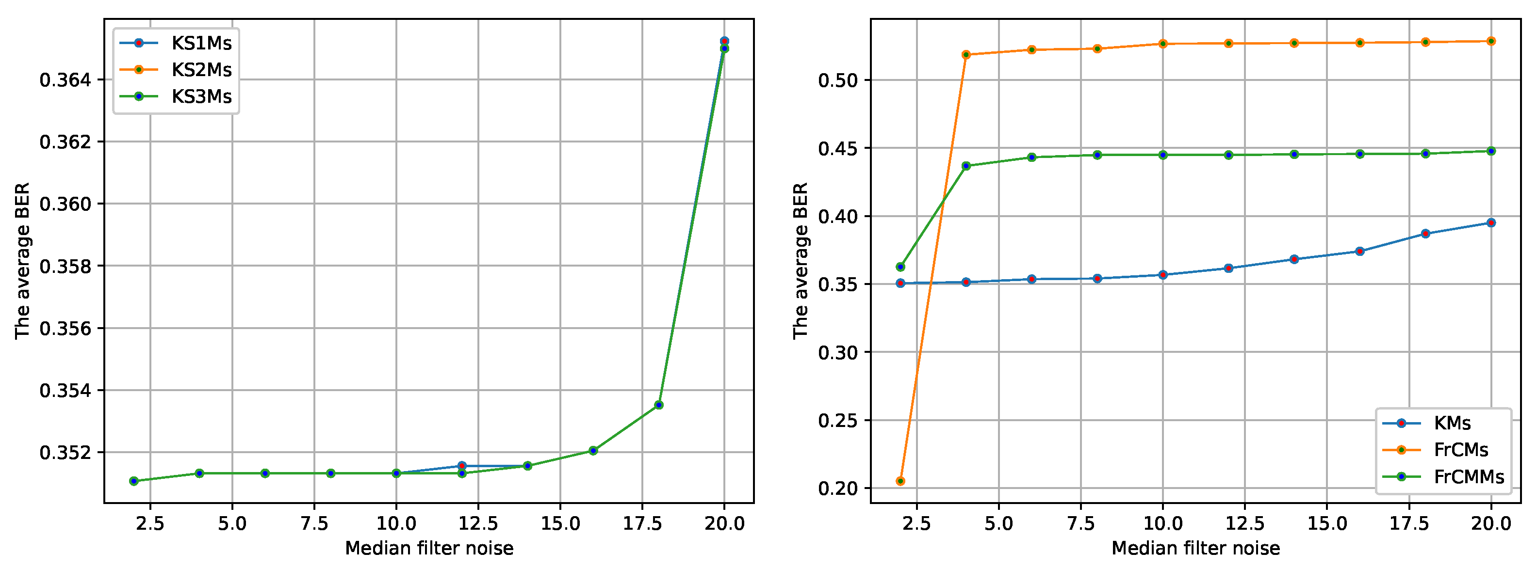
The noises (salt & pepper noise and median filter noise) were more aggressive in all cases, so that the studied moments are less robust to these attacks, see Figure 8 and Figure 11.

6. Discussion

In this work, we have proposed a new procedure to create watermarked images by using Krawtchouk–Sobolev type polynomials. The results obtained undertake a promising future direction of research in which the variation of the parameters involved in the definition of the polynomials can vary in order to give optimal results, compromising a secure watermarking scheme and the similarity of the cover and the watermarked image.

A future work in this direction is to obtain optimized values for the parameters involved in the definition of the Sobolev type polynomials. According to the results obtained, the case of $j=2$ seems to give better results and should be analyzed separately.