Detail-Aware Deep Homography Estimation for Infrared and Visible Image

Abstract

Homography estimation of infrared and visible images is a highly challenging task in computer vision. Recently, the deep learning homography estimation methods have focused on the plane, while ignoring the details in the image, resulting in the degradation of the homography estimation performance in infrared and visible image scenes. In this work, we propose a detail-aware deep homography estimation network to preserve more detailed information in images. First, we design a shallow feature extraction network to obtain meaningful features for homography estimation from multi-level multi-dimensional features. Second, we propose a Detail Feature Loss (DFL), which utilizes refined features for computation and retains more detailed information while reducing the influence of unimportant features, enabling effective unsupervised learning. Finally, considering that the evaluation indicators of the previous homography estimation tasks are difficult to reflect severe distortion or the workload of manually labelling feature points is too large, we propose an Adaptive Feature Registration Rate (AFRR) to adaptive extraction of image pair feature points to calculate the registration rate. Extensive experiments demonstrate that our method outperforms existing state-of-the-art methods on synthetic benchmark dataset and real dataset.

1. Introduction

With the vigorous development of computer vision, single-source images have shown certain limitations. They are difficult to meet the needs of daily applications. In contrast, multi-source images can make up for the lack of single-source image expression capabilities by integrating multi-spectral scene information [1]. Infrared and visible images have been the most widely used image processing [2,3,4]. Infrared images focus on highlighting the overall contour characteristics of the image, and visible images use light to reflect energy on different objects in an image, which can well present scene detail information. They have a high degree of complementarity of scene information [5,6,7,8,9,10,11,12]. Image registration is the process of finding the best alignment between images and plays a very important role in input image preprocessing [13,14,15]. The registration task of infrared and visible images is widely used as an essential part of computer vision applications, such as image fusion [16,17,18] and target tracking [19].

The homography model is mainly used to realize the geometric transformation between two images, including 8 degrees of freedom for scaling, translation, rotation, and perspective, which can be expressed as an image registration problem [20,21,22,23,24]. Traditional feature-based homography estimation methods usually need to detect the features of image pairs [25,26,27,28,29,30,31,32,33,34,35], then establish image correspondences by matching common features, and use robust estimation algorithms such as RANSAC [36] and MAGSAC [37] to eliminate feature correspond to outliers in points. Still, such algorithms require higher quality image pairs. For infrared and visible images, the common features have significant uncertainties, and it is difficult to obtain better registration performance using such methods.

Recent deep homography estimation methods utilize convolutional neural networks to compute the homography matrix between two images [38,39,40,41,42,43,44]. However, most deep learning solutions failed due to the large grayscale and contrast differences inherent in infrared and visible images. At the same time, partial solutions require homography ground-truths for supervised network training, which are often inapplicable in practical applications. In addition, Zhang et al. [40] propose learning deep features and masks to cull outlier regions simultaneously, but this results in loss of details in the image. In practical applications, these details are essential for the image registration task of infrared and visible image, as shown in Figure 1.

In this work, inspired by Zhang et al. [46], we build a feature extraction block by introducing a residual dense network (RDN) to extract detailed information about image pairs. Specifically, we utilize a residual dense network to extract features from both global and local perspectives to generate global perceptual features. In this way, we avoid the defect that most feature extraction methods and ignore hierarchical features, so the resulting features also retain more detailed information.

Since the masks produced in previous methods do not well identify features that are meaningful for homography solving, we construct a feature refinement block. It introduces channel and spatial attention to refine features and suppress unimportant features, thereby retaining meaningful features for homography solving. At the same time, we start from a new direction and generate attention maps directly for the extracted features instead of directly generating masks from the source image and weighting the features as in previous methods [40], which is more conducive to retaining details.

At the same time, since the previous method Triplet Loss [40] loses the details in the image, which are very important for the registration task of infrared and visible images, we propose a new method named “Detail Feature Loss” (DFL) constraints, which directly use the sophisticated features to participate in the loss calculation instead of using the mask [40] in the previous method to normalize the loss. With this improvement, our network preserves more detailed information in image pairs. We describe this in detail in Section 4.6.

In addition, since most of the existing image registration evaluation index functions [47] only use the brightness, contrast, and pixel error of the image to evaluate the image, it is difficult to reflect the registration of severely distorted wrapped images. The point matching error [40,42] uses hand-labelled feature points to calculate the error and is one of the best existing methods to evaluate the registration situation. However, the workload of manual annotation is too large, which results in great difficulties to our evaluation of registration performance, and introduces specific errors. This paper refers to point matching error as PME for short. Moreover, using average corner errors [41,43] to evaluate image registration performance is another suitable method. But this approach only works on synthetic benchmark dataset. This paper refers to the average corner error as ACE for short. Therefore, because of the above difficulties, we design an Adaptive Feature Registration Rate (AFRR) to adaptively extract feature points to calculate the registration performance between image pairs.

Extensive experiments demonstrate that our method outperforms existing state-of-the-art homography estimation methods on synthetic benchmark dataset and real dataset. In summary, our contributions are as follows:

• We design a shallow feature extraction network consisting of a feature extraction block, a feature refinement block, and a feature integration block. The meaningful features are fed into the subsequent network to obtain a homography matrix by performing attention mapping on the channel and spatial dimensions of multi-level features.
• We propose a DFL loss that directly utilizes the sophisticated features to participate in operations to preserve more detailed information in image pairs.
• We propose an image registration evaluation metric, AFRR, to calculate the registration rate of image pairs by adaptively extracting feature points.

2. Related Works

Traditional homography. Image features and feature descriptors are usually first extracted, such as SIFT [25], SURF [26], KAZE [30], ORB [27], BRISK [28], AKAZE [29], and IO-Net [34], and then matched correspondence between common features. Finally, robust estimation algorithms are used to eliminate outliers and solve the homography matrix between image pairs, such as RANSAC [36], MAGSAC [37], and MAGSAC++ [48]. This approach depends heavily on the quality of feature correspondences and tends to fail in infrared and visible image scenes.

Deep homography. Usually, a convolutional neural network is used to obtain the correspondence between image pairs to obtain the homography matrix. DeTone et al. [38] pioneered a VGG-style network for homography estimation that directly learns the parameters of the homography transformation from two images. Nguyen et al. [39] used a photometric loss that does not require manual labels to train the network but failed to converge in infrared and visible image scenarios, making it challenging to achieve registration. Zhang et al. [40] learned a mask to select only reliable regions for homography estimation, which would lose details. Le et al. [41] learn from image pairs with ground-truth homography, which are hard to obtain in practical applications. Shao et al. [43] used a transdoemer structure to address the cross-resolution problem in homography estimation. Nie et al. [44] propose to predict multi-grid homography from global to local to address parallax in images. Inspired by Zhang et al., Ye et al. [42] proposed a homography flow representation to reduce feature rank and suppress motion noise. However, due to the large grayscale and contrast differences between the infrared and visible images, the homography flow is unstable, making it difficult for the network to converge. Similarly, Hong et al. [49] also used homography flow to obtain homography matrices, which would be difficult to apply to infrared and visible scenarios.

Evaluation Metrics. Commonly used image registration evaluation indicators are usually calculated according to the pixels of the image pair, such as SSIM [47], MI [50], PSNR [51], etc. Still, it is difficult to reflect the actual image registration. SSIM and PSNR are also widely used in image denoising tasks and are a general image quality evaluation metric [52,53]. In addition, some evaluation indicators also use location information for evaluation. Ye et al. [42] utilized manually annotated feature points for registration performance evaluation. Specifically, the average $l_2$ distance between the warped source and target points of each pair of test images is considered an error measure. However, this method brings immense workload when the test set data are significant. Le et al. [41] evaluated registration performance by averaging corner errors. Specifically, the method utilizes estimated homography and ground truth homography to transform corners, respectively, which are then used for evaluation index computation. But this method only works on synthetic benchmark dataset.

Discussions. A closely related work to ours is [40], the authors consider using a feature extractor consisting of three layers of convolutions to learn deep features in images and utilize masks to select only reliable regions for homography estimation. Additionally, a Triplet Loss is formulated to enable unsupervised learning. Compared to [40], our work considers the importance of details in the image and retains more details from three aspects. First, RDN [46] is introduced to obtain dense features in the image. Second, CBAM [54] is introduced to refine the features in both channel and space dimensions and transform the location of the attention. Finally, the proposed DFL directly utilizes the refined features to participate in the loss computation.

3. Algorithm

3.1. Network Structure

This section proposes a detail-aware depth homography estimation method for infrared and visible image scenes. Our network consists of two parts: a shallow feature extraction network and a homography estimation network. The shallow feature extraction network consists of a feature extraction block (FEB), a feature refinement block (FRB), and a feature integration block (FIB). Figure 2 shows the basic framework of our network. First, two grayscale image patches $I_a$ and $I_b$ of size $H\times W\times 1$ are given as the input of the neural network, and they are input into the shallow feature extraction network to obtain the integrated refined feature map $G_a$ and $G_b$, respectively. Second, connect the two integrated refined features in the channel dimension to obtain $G_{a,b}$, and input it into the homography estimation network with ResNet-34 [55] as the backbone to get the offset matrix $H$ between the two image pairs. Finally, for the offset matrix $H$, we use direct linear transformation (DLT) [56] to obtain the homography matrix $H_{ab}$ of image pairs, and then calculate the loss to back-propagate the modified network parameters.

3.1.1. Feature Extraction Block

Previous methods [40] cannot extract enough details from the images for infrared and visible images. To address this issue, we introduce RDN [46] to extract multi-level detail information in images to enhance image representation. At the same time, since we want to keep the output feature map size consistent with the input image size, we do not need to upsample the image as in RDN [46], our feature extraction block structure is shown in Figure 3, and Section 4.6 demonstrates in detail the effectiveness. Specifically, given a grayscale image patch of size $H\times W\times 1$ as input. The shallow image features are first extracted through two convolutional layers. Then the dense features in the image are extracted through 3 RDBs. Finally, global fusion is used to preserve the hierarchical features in the image and output a multi-channel feature map of size $H\times W\times 1$. Meanwhile, for grayscale image patches $I_a$ and $I_b$, the network weights are shared to output multi-channel feature maps $F_a$ and $F_b$, i.e.,

$$F_k=F_{\mathrm{-1}}+H_{\mathit{GFF}}\left(\right[F_1,F_2,F_3\left]\right),k\mathsf{\in }\{a,b\}$$

(1)

where $F_{-1}$ denotes the shallow features. $F_d$ depicts the dense features extracted by the d-th RDB, $d\in \left\{1,2,3\right\}$. $H_{GFF}(·)$ means the fusion operation of three RDBs.

3.1.2. Feature Refinement Block

In [40], Zhang et al. use the mask predictor to generate masks directly from the source image, but the network framework of this method is idealization, and the ability to refine features is insufficient. It is difficult to identify the homography matrix solution in a large number of detailed meaningful features. To address this problem, we start from a new direction. Instead of generating attention maps directly for source images, we introduce CBAM [54] to adaptively refine the features themselves. Specifically, the detailed features are further refined by sequentially extracting informative features along the two dimensions of channel and space by mapping multi-channel features $F_k$ to focus on the most critical features and suppress unimportant features. Similar to the feature extraction block, for the multi-channel feature maps $F_a$ and $F_b$, the feature refinement block shares weights and outputs of size $H\times W\times C$ the refined feature map $M_a$ and $M_b$, i.e.,

$$\begin{array}{c}{M}_k^{\prime }=M_{ck}\left(F_k\right)\otimes F_k\\ M_k=M_{sk}\left(M_k^{\prime }\right)\otimes M_k^{\prime }\end{array},k\in \left\{a,b\right\}$$

(2)

where $M_{ck}\in R^{C\times 1\times 1}$ and $M_{sk}\in R^{1\times H\times W}$ denote the channel attention map and the spatial attention map, respectively.

3.1.3. Feature Integration Block

Since the number of output channels of the feature extraction block and the feature refinement block are both $C$, this increases the time and computational complexity of the subsequent homography estimation network training. We design a feature integration block to transform the number of channels of the feature map to 1. Specifically, our feature integration block consists of two convolutional layers, and each convolutional layer is followed by batch normalization [57] and ReLu, as shown in

Table 1. Feature integration blocks.

Layer	1	2
Type	Conv	Conv
Kernel	3	3
Stride	1	1
Channel	32	1

. Similar to the feature extraction block, the feature integration block takes a feature map of size $H\times W\times C$ as input, and the shared network weight outputs an integrated feature map of size $H\times W\times 1$, i.e.,

$$G_k=f\left(M_k\right),k\in \left\{a,b\right\}$$

(3)

where $G_k$ depicts the integrated refined feature map. $f(·)$ represents the operation of the feature integration block.

3.2. Triplet Loss with Retaining Details

In the visible image scene, although the Triplet Loss [40] can use the mask as a weighting term to make the network pay more attention to the regions suitable for alignment, for the homography estimation of infrared and visible images, this method loses the detailed information in the image degrades the registration performance. This paper starts from a new perspective by proposing a constraint named “Detail Feature Loss” (DFL), which uses the integrated refined feature map to participate in the loss calculation. Specifically, since it is difficult for a single homography to satisfy the transformation between two views in real scenes, the previous Triplet Loss [40] uses masks for normalization. Based on this inspiration, we use the integrated refined features to calculate the loss, which can preserve many details while reducing the influence of unimportant features. We demonstrate this in Section 4.6.

According to the homography matrix $H_{ab}$ obtained by the network, image $I_a$ can be wrapped into $I_a^{\prime }$, and our DFL can be expressed as:

$$L_T\left(I_a^{\prime },I_b\right)=||G_a^{\prime }-G_b{||}_1-||G_a-G_b{||}_1$$

(4)

where $G_a^{\prime }$ is the integrated refined feature produced by the warped image $I_a^{\prime }$.

In practice, we also swap the order of the network input image pairs $I_a$ and $I_b$ to produce a homography matrix $H_{ba}$, resulting in a warped image $I_b^{\prime }$ of $I_b$. Similar to Equation (4), another loss $L_T\left(I_b^{\prime },I_a\right)$ is obtained. At the same time, we force $H_{ab}$ and $H_{ba}$ to be inverses of each other. Therefore, our objective function is as follows:

$$L=L_T\left(I_a^{\prime },I_b\right)+L_T\left(I_b^{\prime },I_a\right)+\lambda ||H_{ab}{H}_{ba}-E{||}_2^2$$

(5)

where $\lambda$ denotes the equilibrium hyperparameter, which is set to 0.01 in the experiments. $E$ is a third-order identity matrix.

3.3. Adaptive Feature Registration Rate

SSIM, MI, and PSNR are currently the most widely used image evaluation metrics. Image registration tasks are generally sensitive to grayscale changes and suffer from distorted wrapped images and black edges. At the same time, their evaluation values are often difficult to reflect accurately under these interferences. They have a large deviation from the observation results of human eyes, so these indicators often cannot reflect the actual registration performance. We perform a detailed experimental proof in Section 4.6. Meanwhile, another evaluation method has recently been widely used in image registration tasks, namely, PME [40]. Compared with other methods, this method can better reflect the registration situation but often requires manual annotation of feature points. For a test set with a large amount of data, the labor cost of this method is too high. In addition, the ACE [41] is also widely used in image registration tasks, but this evaluation metric can only be applied to synthetic benchmark dataset containing ground-truth values.

According to the above observations, we directly use SIFT [25] to adaptively extract feature points from another perspective and use the ratio of more accurate feature points as the evaluation value to obtain the Adaptive Feature Registration Rate (AFRR). At the same time, the use of feature points for evaluation calculation can effectively avoid problems such as registration performance and manual annotation workload that are difficult to reflect in other evaluation indicators. Specifically, we first adaptively extract feature points of image pairs by SIFT [25] and utilize FLANN [58] to match feature corresponding points. Then, the Euclidean distance $d_i$ between the feature corresponding points (representing the i-th feature corresponding point) is used as the judgment amount. Since SIFT [25] itself may have mismatches, we need to remove the mismatched points corresponding to the feature points. The specific method is as follows: we select a threshold value $\epsilon$ as the judgment criterion for mismatching, that is, only $d_i$ smaller than the threshold value $\epsilon$ is included in the subsequent judgment range. We denote $d_i$ that falls within this range as $d_i^{\prime }$.

In addition, we also set a threshold of $\mu$, if and only if $d_i^{\prime }$ is less than $\mu$, and we record the corresponding point of the feature as a feature point with more accurate registration. On the contrary, it is recorded as the feature points whose registration is inaccurate. Finally, the registration rate is generated by calculating the number of accurately registered feature points within the judgment range, and this is used as the evaluation value of AFRR. Therefore, our calculation formula is as follows:

$$\mathrm{AFRR}=\frac{1}{N}{\displaystyle \sum }_{i=1}^N{d}_i^{\prime }$$

(6)

where $N$ denotes the corresponding number of feature points that satisfy the threshold $\epsilon$. We set the threshold $\epsilon$ to 10 and the threshold $\mu$ to 6 respectively in our experiments.

4. Experiment

4.1. Dataset and Implementation Details

4.1.1. Dataset

Synthetic benchmark dataset. We validate our algorithm on synthetic benchmark dataset and real dataset, respectively. We make our synthetic benchmark dataset from publicly registered infrared and visible datasets such as OSU Color-Thermal Database [59], INO [60], and TNO [61]. We selected 115 pairs and 42 pairs of infrared and visible images for training and test sets, respectively.

Real dataset. The real dataset comes from the KAIST multispectral pedestrian detection dataset [62]. Although it is stated that the infrared and visible images are already aligned in [62], there is an offset in the case of camera movement. We only select image pairs with camera movement for the dataset. Finally, we selected 80,189 pairs of infrared and visible images for the training set, and 49 pairs of infrared and visible images for the test set.

4.1.2. Implementation Details

The experimental configuration is an Intel i9-10980XE processor, 64G memory, and NVIDIA GeForce RTX 3090 GPU. The deep learning framework we adopt is Pytorch, and Adam is used as the network optimizer. The exponential decay learning rate is initialized to 1.0 × 10⁻⁴, the decay factor is 0.8, and the decay step size is 1 epoch. The batch size is set to 16, and the epoch is set to 50.

4.2. Experiment Procedure

The experiment procedure is divided into three steps. In step 1, the data are augmented to construct a dataset for experiments. In step 2, the image data are normalized to obtain the network input image. In step 3, we visualize the network output results of the feature extraction block, feature refinement block, and feature integration block in turn according to the proposed framework, and finally display the distorted image transformed by the homography matrix.

4.2.1. Data Augmentation

Synthetic benchmark dataset. First, because of the problem of too little data in the training set, we use data augmentation methods such as rotation, offset, and clipping to expand. To use the same parameters for augmentation, we uniformly transform the training set images of different sizes to 320 × 240. A total of 48,736 infrared and visible image pairs are obtained. Second, we use the dataset generation method in [38] on the training and test set to generate synthetic benchmark dataset. The synthetic benchmark dataset includes infrared image $I_r$, visible image $I_v$, and infrared ground-truth image $I_{GT}$ of size 150 × 150, where $I_r$ and $I_v$ are unregistered, and $I_v$ and $I_{GT}$ are registered. In particular, only $I_{GT}$ is included in the test set, which is intended to be used for evaluation index calculation, so as to better reflect the registration performance of infrared and visible images. The specific production method of the synthetic benchmark dataset is shown in Figure 4. The comparative information of the original dataset and the synthetic benchmark dataset is shown in

Table 2. Comparative information of the original dataset and the synthetic benchmark dataset. The source image column indicates the number and resolution of images used in different subsets or categories in the source dataset (OSU Color-Thermal Database, INO, and TNO). The unregistered image column indicates the number and resolution of images in different subsets or classes in the synthetic benchmark dataset.

	Dataset	Subsets/Categories	Original Image		Unregistered Image
			Number	Resolution	Number	Resolution
Training set	OSU Color-Thermal Database	Location 1	10	320 × 240	3383	150 × 150
	INO	Close person	2	512 × 184	841	150 × 150
		Coat deposit	14	512 × 384	6093	150 × 150
		Group fight	18	452 × 332	7773	150 × 150
		Main entrance	9	328 × 254	3975	150 × 150
		Multiple deposit	5	448 × 324	2261	150 × 150
		Parking evening	6	328 × 254	2598	150 × 150
		Trees and runner	5	328 × 254	2165	150 × 150
		Visitor parking	9	328 × 254	3732	150 × 150
	TNO	Athena	14	768 × 576, 595 × 328 etc.	5959	150 × 150
		DHV	2	280 × 280	780	150 × 150
		FEL	2	360 × 270	837	150 × 150
		tank	1	472 × 354	455	150 × 150
		Triclobs	18	640 × 480, 620 × 458 etc.	7884	150 × 150
Test set	OSU Color-Thermal Database	Location 2	9	320 × 240	9	150 × 150
	INO	Parking snow	16	448 × 324	16	150 × 150
		Backyard runner	4	448 × 324	4	150 × 150
	TNO	Athena	2	590 × 426, 768 × 576	2	150 × 150
		DHV	1	575 × 475	1	150 × 150
		Triclobs	10	472 × 371, 622 × 458 etc.	10	150 × 150

.

Real dataset. The brightness of the infrared images in the multispectral pedestrian dataset is too dark, so we also enhanced the contrast of the infrared images by employing image enhancement as our final dataset, as shown in Figure 5. In particular, the enhanced real dataset is the size of 200 × 200. The comparison information between the original dataset and the enhanced real dataset is shown in

Table 3. Comparison information of the original dataset and the enhanced real dataset. The source image column indicates the number and resolution of images used in different subsets or categories in the source dataset (KAIST multispectral pedestrian detection dataset). The enhanced image column indicates the number and resolution of images in different subsets or categories in the real dataset after enhancement.

	Dataset	Subsets/Categories	Original Image		Enhanced Image
			Number	Resolution	Number	Resolution
Training set	KAIST multispectral pedestrian detection dataset	Day Campus	28,104	640 × 512	28,104	200 × 200
		Day Road	12,509	640 × 512	12,509	200 × 200
		Day Downtown	14,212	640 × 512	14,212	200 × 200
		Night Campus	6668	640 × 512	6668	200 × 200
		Night Road	12,270	640 × 512	12,270	200 × 200
		Night Downtown	6426	640 × 512	6426	200 × 200
Test set	KAIST multispectral pedestrian detection dataset	Day Campus	16	640 × 512	16	200 × 200
		Night Campus	33	640 × 512	33	200 × 200

.

4.2.2. Data Normalization

Due to the different image sizes in different datasets, we uniformly transform the images to 150 × 150 in the network preprocessing. Then, we also get normalized grayscale images by normalization and gray scale. Finally, an image patch of size 128 × 128 is randomly generated from the grayscale image as the input image of the subsequent network to enhance the richness of the dataset. It is worth noting that uniform downsampling or upsampling of images of different sizes to fixed-size images will blur or introduce noise into the network input image in the above process.

4.2.3. Network Layer Output

To clearly show the results of data processing in the network layer, we visualized the network output results of the feature extraction block, feature refinement block, and feature integration block on the synthetic benchmark dataset, respectively. The results are shown in Figure 6. In particular, since the outputs of both the feature extraction block and feature refinement block are multi-channel feature maps, we only visualize their first channel.

First, we perform feature extraction on the input images $I_a$ and $I_b$ using a feature extraction block, respectively, to generate multi-channel feature maps $F_a$ and $F_b$, and the results are shown in column 2 in Figure 6. We can see that the feature extraction block can obtain richer detailed features. Second, we use the feature refinement block to refine the input multi-channel feature maps $F_a$ and $F_b$, respectively, to obtain the refined feature maps $M_a$ and $M_b$, and the results are shown in the third column in Figure 6. The road edge features and pedestrian features in the lower left corner of $M_a$ are significantly less than those in $F_a$, and the pedestrian head features in the lower left corner of $M_b$ are also significantly less than those in $F_b$, which fully shows that the feature refinement block is important to refine the feature in $F_a$ and $F_b$. Finally, we integrate the multi-channel refined features in $M_a$ and $M_b$ using a feature integration block to produce single-channel integrated refined feature map $G_a$ and $G_b$. This reduce the time and computation for subsequent homography estimation network training, and the results are shown in column 4 in Figure 6. After integrating the refined features of multiple channels, our single-channel feature map $G_a$ and $G_b$ are fine and dense.

In addition, we input $G_a$ and $G_b$ into the homography estimation network after channel concatenation to obtain the final homography matrix. The warped image produced by transforming the source image by the homography matrix is shown in Figure 7, where $I_{GT}$ represents the infrared image form corresponding to the visible target image. As shown in Figure 7, we can see that the warped image is closer to the target image than the source image, which confirms the accuracy of the homography matrix.

4.3. Evaluation Metrics

SSIM [47] uses the brightness, contrast, and structure of the image to measure the image similarity, and its value belongs to [0, 1]. The larger the value of SSIM, the better the registration effect. The calculation formula can be described as:

$$\mathrm{SSIM}\left(x,y\right)=\frac{\left(2{\mu }_x{\mu }_y+C_1\right)\left(2{\sigma }_{xy}+C_2\right)}{\left({\mu }_x^2+{\mu }_y^2+C_1\right)\left({\sigma }_x^2+{\sigma }_y^2+C_2\right)}$$

(7)

where $x$ and $y$ denote warped and ground-truth images, respectively. ${\mu }_x$ and ${\mu }_y$ represent the mean of all pixels in $x$ and $y$, respectively. ${\sigma }_x$ and ${\sigma }_y$ represent the standard deviations of $x$ and $y$, respectively. ${\sigma }_{xy}$ represents the covariance of the two images. $C_1$ and $C_2$ represent constants to maintain stability.

MI [50] reflects the degree of correlation by calculating the entropy and joint entropy of both the warped and ground-truth images. The larger the value, the higher the similarity. The calculation formula of MI can be described as:

$$\mathrm{MI}\left(x,y\right)=\mathrm{H}\left(\mathrm{x}\right)+\mathrm{H}\left(\mathrm{y}\right)-\mathrm{H}\left(\mathrm{x},\mathrm{y}\right)$$

(8)

where $x$ and $y$ denote warped and ground-truth images, respectively. $\mathrm{H}(·)$ and $\mathrm{H}\left(x,y\right)$ denote the calculation functions of entropy and joint entropy, respectively.

PSNR [51] can directly reflect the difference in the grayscale of the two images as a whole. The larger the PSNR value, the smaller the gray difference between the two images, that is, the more similar the image pair is. The calculation formula of PSNR is as follows:

$$\mathrm{PSNR}\left(x,y\right)=10lo{g}_{10}\frac{MN{\left(2^k-1\right)}^2}{{{\displaystyle \sum }}_{i=1}^M{{\displaystyle \sum }}_{j=1}^N{\left(x\left(i,j\right)-y\left(i,j\right)\right)}^2}$$

(9)

where $x$ and $y$ denote warped and ground-truth images, respectively. $i$ and $j$ represent the pixel locations in the image row and column, respectively. $k$ is the number of bits per sample value.

Average corner error (ACE) [41,43] evaluates the homography performance by transforming the corners with estimated and ground-truth homography, respectively. The smaller the ACE value, the better the homography estimation performance, that is, the better the registration performance. The calculation formula of ACE can be expressed as:

$$\mathrm{ACE}=\frac{1}{4}{{\displaystyle \sum }}_{j=1}^4||x_j-y_j{||}_2$$

(10)

where $x_j$ and $y_j$ are the corner $j$ transformed by the estimated homography and the ground-truth homography, respectively.

Point matching error (PME) [40,42] utilizes manually annotated feature points for homography estimation performance evaluation, and it regards the average l2 distance between warped source and target points for each pair of test images as an error metric. The smaller the PME value, the better the homography estimation performance, that is, the better the registration performance. The calculation formula of PME is as follows:

$$\mathrm{PME}=\frac{1}{N}{{\displaystyle \sum }}_{j=1}^N||x_j-y_j{||}_2$$

(11)

where $x$ denotes the feature points produced by the estimated homography transformation. $y$ represents the target feature point marked manually. $N$ represents the number of manually labeled feature point pairs.

4.4. Comparison on Synthetic Benchmark Dataset

We conduct quantitative comparisons with 11 algorithms on synthetic benchmark dataset, including traditional feature-based methods and deep learning-based methods. The evaluation results on warped infrared images and infrared ground-truth images are shown in

Table 4. Quantitative comparison on synthetic benchmark dataset. We mark the best method in red and the suboptimal method in blue. The rest of this article uses the same notation method.

(1)		SSIM (↑)	MI (↑)	PSNR (↑)	ACE (↓)	AFRR (↑)
(2)	I3×3	0.54 (+0.00%)	1.09 (+0.00%)	30.66 (−0.16%)	5.79 (+10.29%)	0.73 (−23.96%)
(3)	SIFT + RANSAC	0.49 (−9.26%)	0.95 (−12.84%)	30.01 (−2.28%)	50.87 (+868.95%)	0.96 (+0.00%)
(4)	SIFT + MAGSAC++	0.45 (−16.67%)	0.88 (−19.27%)	29.58 (−3.68%)	131.71 (+2408.76%)	0.65 (−32.29%)
(5)	ORB + RANSAC	0.36 (−33.34%)	0.59 (−45.87%)	28.17 (−8.27%)	160.89 (+2964.57%)	0.05 (−94.79%)
(6)	ORB + MAGSAC++	0.36 (−33.34%)	0.56 (−48.62%)	28.14 (−8.37%)	109.13 (+1978.67%)	0.06 (−93.75%)
(7)	KAZE + RANSAC	0.34 (−37.04%)	0.63 (−42.20%)	28.40 (−7.52%)	144.07 (+2644.19%)	0.09 (−90.63%)
(8)	KAZE + MAGSAC++	-	-	-	-	-
(9)	BRISK + RANSAC	0.36 (−33.34%)	0.57 (−47.71%)	28.21 (−8.14%)	143.20 (+2627.62%)	0.03 (−96.87%)
(10)	BRISK + MAGSAC++	0.36 (−33.34%)	0.58 (−46.79%)	28.18 (−8.24%)	146.62 (+2692.76%)	0 (−100.00%)
(11)	AKAZE + RANSAC	0.28 (−48.15%)	0.55 (−49.54%)	28.15 (−8.34%)	159.66 (+2941.14%)	0 (−100.00%)
(12)	AKAZE + MAGSAC++	0.26 (−51.85%)	0.57 (−47.71%)	28.14 (−8.39%)	139.40 (+2555.24%)	0 (−100.00%)
(13)	CADHN	0.54 (+0.00%)	1.09 (+0.00%)	30.71 (+0.00%)	5.25 (+0.00%)	0.73 (−23.96%)
(14)	Proposed method	0.55 (+1.85%)	1.10 (+0.97%)	30.74 (+0.10%)	5.08 (−3.24%)	0.74 (−22.92%)

. In Table 4, I_3×3 indicates that the 3 × 3 identity matrix is used as the “no-warping” homography matrix, and “-” indicates that the algorithm fails. We used evaluation metrics such as SSIM, MI, PSNR, ACE [41], and AFRR in the quantitative comparison. Since MSE is calculated similarly to ACE [41] and PME [40], we do not use it as our evaluation metric in the future. In particular, partial deep learning-based methods are difficult to fit on infrared and visible datasets, such as UDHN [39], MBL-UDHEN [42], etc.

As shown in Table 4, our algorithm significantly outperforms feature-based methods on most of the evaluation metrics, only worse than SIFT [25] + RANSAC [36] on the evaluation metric AFRR. Although this class of methods achieves the best on AFRR, it is the algorithm with the highest failure rate except for KAZE [30] + MAGSAC++ [48], as shown in Figure 8. This shortcoming will greatly limit the practical application, and the rest of the traditional methods usually suffer from algorithm failures on infrared and visible datasets. In addition, we can observe that the ACE [41] of the traditional method is generally large, which is caused by the characteristic of calculating the evaluation value through the corner position, so the size of the evaluation value reflects the degree of distortion of the image.

Furthermore, our algorithm slightly outperforms CADHN [40] on every evaluation metric. In particular, the algorithm performance is significantly improved by 3.24% on ACE [41].

4.5. Comparison on Real Dataset

Qualitative comparison. We performed qualitative comparisons with 11 contrasting algorithms on real dataset and fused the blue and green channels of the visible warped image with the red channel of the infrared target image to evaluate the registration performance. The fusion results are shown in Figure 9, where “-” indicates that the algorithm fails. We can see that the feature-based solutions are severely distorted, and the algorithm is prone to failure. Therefore, it is difficult for the feature-based method to obtain a more accurate homography matrix in infrared and visible scenarios. In particular, the KAZE [30] + MAGSAC++ [48] algorithm fails on the test set.

In addition, the deep learning-based solution significantly outperforms the feature-based solution, resulting in more accurate warped images. Although it is difficult to see a significant difference between our method and CADHN [40] in qualitative comparison, according to the PME [40] in the lower right corner of Figure 9, our results in both examples are significantly better than CADHN [40]. The PME [40] drops significantly from 4.04 and 5.86 to 3.43 and 5.19, respectively, where the red ghost in the fusion result of our method and CADHN [40] represents the texture in the infrared target image.

Quantitative comparison. We use evaluation metrics such as SSIM, MI, PSNR, PME [40], and AFRR to quantitatively compare visible warped images with infrared target images to demonstrate the effectiveness of our method, as shown in

Table 5. Quantitative comparison on real dataset.

(1)		SSIM (↑)	MI (↑)	PSNR (↑)	PME (↓)	AFRR (↑)
(2)	I3×3	0.17 (−55.26%)	0.90 (+0.00%)	27.90 (+0.00%)	5.01 (+16.24%)	0.08 (−27.27%)
(3)	SIFT + RANSAC	0.38 (+0.00%)	0.44 (−51.11%)	27.72 (−0.65%)	226.60 (+5157.54%)	0 (−100.00%)
(4)	SIFT + MAGSAC++	0.16 (−57.90%)	0.53 (−41.11%)	27.63 (−0.97%)	180.05 (+4077.49%)	0 (−100.00%)
(5)	ORB + RANSAC	0.15 (−60.53%)	0.61 (−32.22%)	27.96 (−0.22%)	153.46 (+3460.56%)	0 (−100.00%)
(6)	ORB + MAGSAC++	0.15 (−60.53%)	0.58 (35.56%)	27.95 (−0.18%)	128.93 (+2891.42%)	0 (−100.00%)
(7)	KAZE + RANSAC	0.14 (−63.16%)	0.52 (−42.22%)	28.00 (−0.36%)	417.28 (+9581.67%)	0 (−100.00%)
(8)	KAZE + MAGSAC++	-	-	-	-	-
(9)	BRISK + RANSAC	0.16 (−57.90%)	0.57 (−36.67%)	27.93 (−0.11%)	163.84 (+3701.39)	0.01 (−90.91%)
(10)	BRISK + MAGSAC++	0.16 (−57.90%)	0.54 (−40.00%)	27.93 (−0.11%)	139.85 (+3144.78%)	0 (−100.00%)
(11)	AKAZE + RANSAC	0.14 (−63.16%)	0.62 (−31.11%)	27.98 (−0.29%)	149.33 (+3364.73%)	0 (−100.00%)
(12)	AKAZE + MAGSAC++	0.15 (−60.53%)	0.56 (37.78%)	27.97 (−0.25%)	122.65 (+2745.71%)	0 (−100.00%)
(13)	CADHN	0.17 (−55.26%)	0.89 (+1.11%)	27.90 (+0.00%)	4.31 (+0.00%)	0.11 (+0.00%)
(14)	Proposed method	0.16 (−57.90%)	0.88 (−2.22%)	27.90 (+0.00%)	4.14 (−3.94%)	0.16 (+45.46%)

. Infrared and visible image pairs have large grayscale differences, so evaluation metrics based on the pixel values are no longer applicable to this task. As shown in Table 5, despite the severe distortion of the feature-based solutions, their SSIM and PSNR are consistent with the neural network-based methods, and even the PSNR of most of the feature-based methods is slightly higher than that of the neural network-based methods, which is obviously unrealistic.

In addition, MI measures the correlation between sets, so it can better reflect the registration performance than SSIM and PSNR. However, MI is also affected by image pixel values, so it cannot accurately express the image registration performance, nor can it reflect the registration performance of severely distorted wrapped images. Only a rough evaluation can be made. As can be seen from Table 5, the deep learning-based solution significantly outperforms the feature-based solution.

Since the PME [40] is calculated based on the position of the feature points, it is not affected by the gray level, which can well reflect the accuracy of the predicted homography matrix. As in column 5 in Table 5, the feature-based solution cannot estimate a more accurate homography matrix, and the neural network-based solution performs well. In particular, since our method pays more attention to the details in the image pair, the performance of PME [40] is improved by 3.94%.

As shown in column 6 in Table 5, the AFRR evaluation value of the feature-based methods is 0, which is consistent with the severe distortion they appear in the qualitative comparison. In particular, our method significantly outperforms CADHN [40] with a significant improvement in AFRR performance from 0.11 to 0.16. Although our evaluation metric AFRR can distinguish the registration performance of different algorithms to a certain extent, its accuracy is not high enough. This is because it has the defect of SIFT [25], that is, it is difficult to extract feature point pairs of better quality in heterologous image pairs, which affects the calculation of AFRR itself.

4.6. Ablation Studies

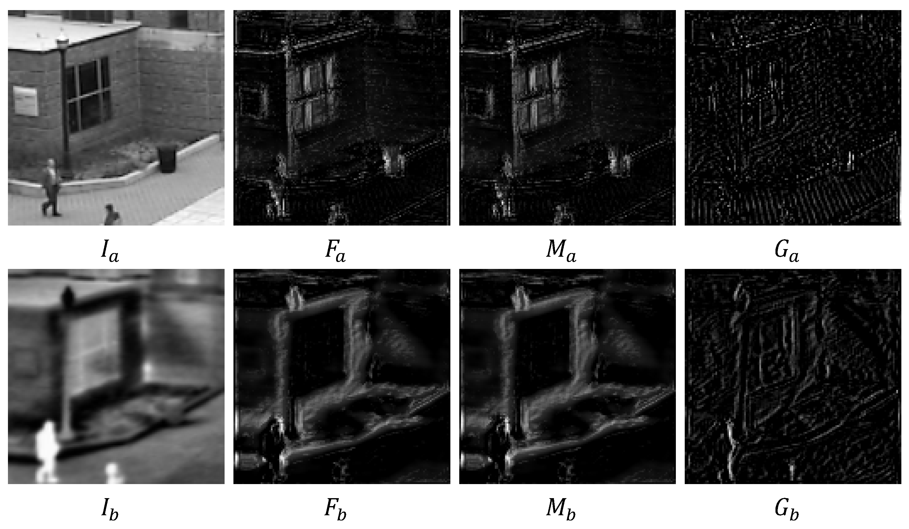
Feature extraction block. We conduct ablation experiments on a synthetic benchmark dataset and verify its effectiveness by replacing the feature extractor in [40] with the feature extraction block and feature integration block in our model. The main reason for adding a feature integration block is to keep the number of output channels of the feature extractor in [40] consistent. In Figure 10, we visualize the feature extraction results of these two methods. According to the observation, compared with the feature extractor of [40], the feature extraction block can extract the deep-level features in the image, and the outline is more precise. As shown in rows 2 and 3 in

Table 6. Ablation experiments.

(1)		SSIM (↑)	MI (↑)	PSNR (↑)	ACE(↓)	AFRR (↑)
(2)	Feature extractor [40]	0.54 (−1.82%)	1.09 (−0.91%)	30.71 (−0.10%)	5.25 (+3.35%)	0.73 (−1.35%)
(3)	Feature extraction block & Feature integration block	0.54 (−1.82%)	1.09 (−0.91%)	30.72 (−0.07%)	5.19 (+2.17%)	0.73 (−1.35%)
(4)	Backshift mask predictor	0.54 (−1.82%)	1.09 (−0.91%)	30.70 (−0.13%)	5.15 (+1.38 %)	0.73 (−1.35%)
(5)	Triplet Loss [40]	0.54 (−1.82%)	1.09 (−0.91%)	30.73 (−0.03%)	5.13 (+0.98%)	0.73(−1.35%)
(6)	DFL	0.55	1.10	30.74	5.08	0.74

, the evaluation metric ACE [41] drops significantly from 5.25 to 5.19, but the remaining four evaluation metrics are basically unchanged. The main reason is that the evaluation metric ACE [41] is calculated on the wrapped source and target points, so it has a high sensitivity to small changes in the image. However, due to the calculation characteristics of the rest of the evaluation indicators, the subtle changes in the image cannot be clearly reflected. In the subsequent ablation experiments of the evaluation metric AFRR, we explain it in more detail.

Feature refinement block. We demonstrate its effectiveness from both the location of the feature refinement block and itself. First, we show that the performance of generating attention maps directly from features is slightly better than that of generating attention maps from the images themselves. Specifically, we modified the position of the mask predictor to the “Feature extraction block & Feature integration block” and then compared it with the “Feature extraction block & Feature integration block” to prove the importance of the position. The result is shown in row 4 in Table 6. We can see that ACE [41] drops significantly from 5.25 to 5.19, and the rest of the evaluation metrics remain unchanged.

Second, we replace the mask predictor in the network framework of the “Backshift mask predictor” with our feature refinement block and modify its position to be in the middle of the feature extraction block and feature integration block to demonstrate the effectiveness of the feature refinement block. The main reason for modifying the position is that we need to perform attention mapping on the channel and space dimensions, and the original number of output channels is 1, which obviously cannot meet our needs. The comparison results are shown in rows 4 and 5 in Table 6. We can see that the ACE [41] drops significantly from 5.15 to 5.13, and the rest of the evaluation indicators remain unchanged. This shows that the feature refinement block can improve the network performance to a certain extent.

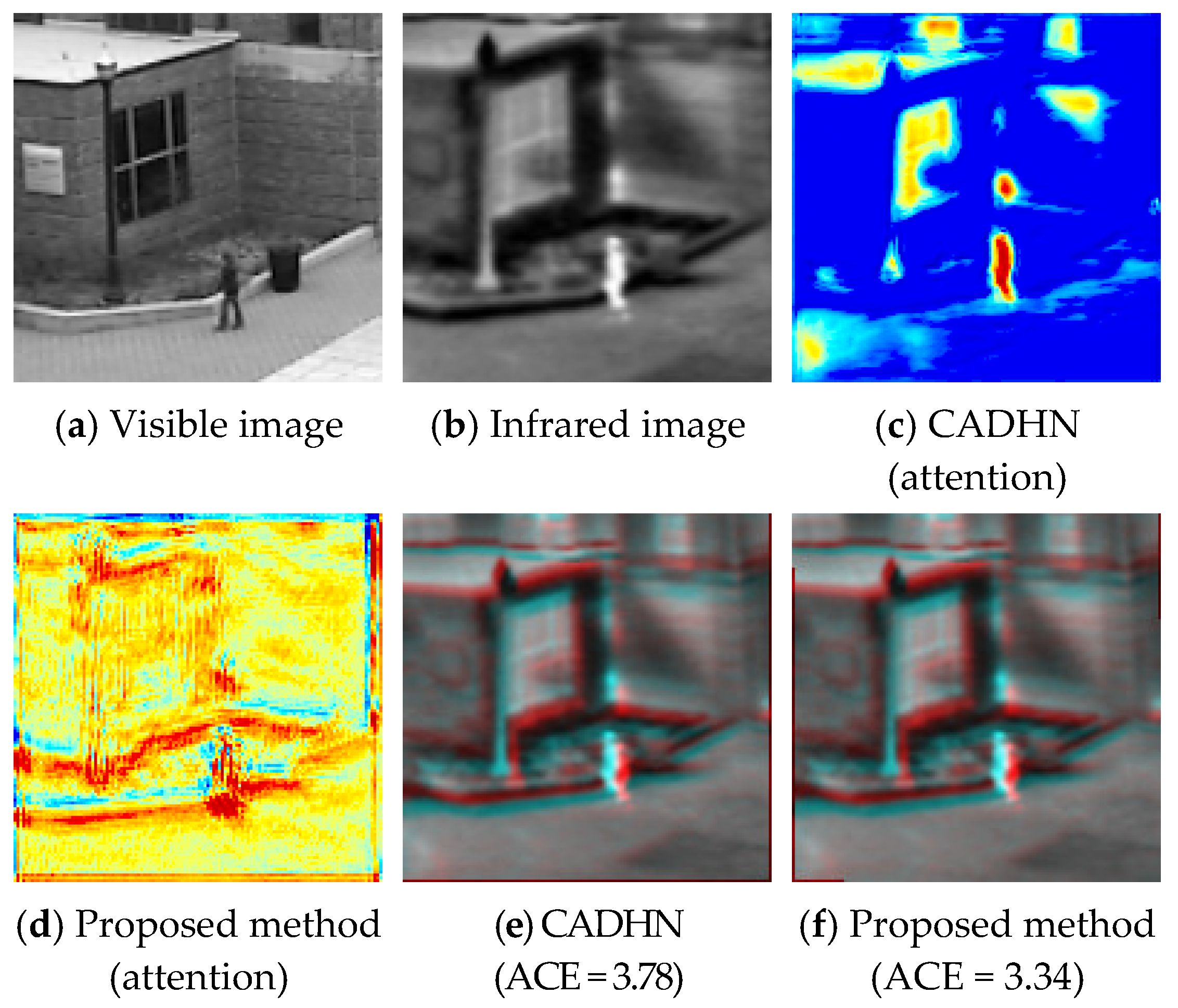
In addition, for a more intuitive understanding of the performance of the feature refinement block, we use Grad-CAM [45] to visualize the attention maps produced in the feature refinement block. The results are shown in Figure 11. Since the attention map in “Feature extraction block & Feature integration block” is generated from the original grayscale image, the other two comparison algorithms are generated from the feature map of the image patch, the visual image content of these two algorithms is less than “Feature extraction block & Feature integration block”. As shown in columns 2 and 3 in Figure 11, compared to “Feature extraction block & Feature integration block”, “Backshift mask predictor” focuses more on the image features themselves but cannot identify deep-level features in the image. But as shown in column 4 in Figure 11, after introducing the feature refinement block, not only the features can be refined, but also more deep-level features can be extracted.

DFL. To demonstrate the effectiveness of our proposed DFL, we compare by modifying the DFL in our network to “Triplet Loss” in [40]. The results are shown in Table 6 and Figure 12. According to the visualization results in Figure 12, we can see that the proposed loss can retain more detailed information by using the integrated refined features to calculate. According to rows 5 and 6 in Table 6, the proposed loss can effectively improve the performance of the network, especially for SSIM and AFRR, the performance is improved by 1.82% and 1.35%, respectively. In summary, the detailed information can help improve the homography estimation performance between infrared and visible images.

Evaluation indicator AFRR. To demonstrate the effectiveness of the proposed evaluation metrics, we explain them from two perspectives. First, we use ORB [27] and SIFT [25] as the feature point extraction algorithm in AFRR, respectively, to demonstrate the effectiveness of the used feature point extraction algorithm. Figure 13 shows the number of feature corresponding points extracted by ORB [27] and SIFT [25] on 42 pairs of warped images and ground-truth images, where the proposed algorithm predicts the warped images. As shown in Figure 13, the overall trend of the number of feature-corresponding points of ORB [27] and SIFT [25] is consistent, but the number of feature-corresponding points of SIFT [25] is significantly more than that of ORB [27]. In addition, we can see that ORB [27] cannot match the feature corresponding points on the three image pairs clearly, but the warped images in these three image pairs are not severely distorted. Therefore, ORB [27] is often not applicable in practical evaluation scenarios.

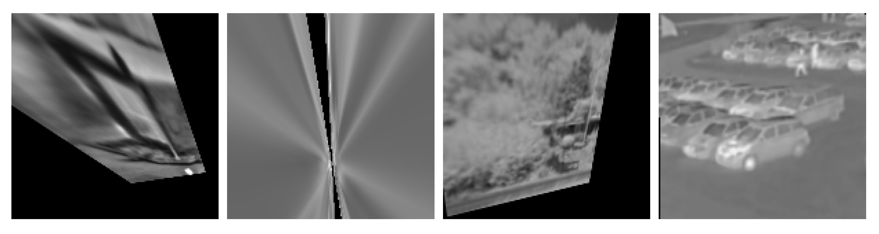
In addition, for infrared and visible images, the homography estimation often produces severely distorted wrapped images in traditional algorithms, so we randomly selected the four group results from ORB [27] + RANSAC [36] and the algorithm in this paper. Four groups of wrapped images and ground-truth images are used to compare different evaluation metrics, thus proving the effectiveness of AFRR, including severely distorted and well-performing wrapped images. The results are shown in Figure 14.

Table 7. Comparison of evaluation indicators of four groups of images.

	SSIM (↑)	MI(↑)	PSNR (↑)	ACE (↓)	AFRR (↑)
(a)	0.10	0.67	27.88	137.70	0
(b)	0.45	0.39	28.37	87.36	0
(c)	0.26	0.52	28.89	34.71	0.57
(d)	0.59	1.02	31.10	4.83	0.92

shows the results of the four groups of images on various evaluation indicators, in which SSIM and PSNR are easily affected by the black background that does not belong to the original image content. MI reflects the registration effect to a certain extent, but cannot more accurately reflect the registration results of severely distorted wrapped images, as shown in (b) in Figure 14 and in row 3 and column 3 of Table 7. In addition, since ACE [41] is obtained from the corners transformed by the estimated homography and ground truth homography, respectively, the estimated value is higher for images with severe distortion and a large number of black backgrounds. This method directly calculates the corner coordinates, so it is more sensitive to image changes, and its accuracy is significantly better than other evaluation indicators, but it is only suitable for synthetic benchmark dataset with ground truth. In short, compared with other evaluation indicators, AFRR can more accurately identify distorted wrapped images and more accurately estimate the registration rate of images, which is more in line with the feeling of the human eye. In particular, due to the computational characteristics of AFRR itself, its accuracy is slightly worse than that of ACE [41].

5. Conclusions

For infrared and visible scenes, we propose a new detail-aware deep homography solution, which includes two components to improve the performance of previous methods: a shallow feature extraction network to extract multi-level and multi-dimensional fine features to improve homography estimation performance and a Detail Feature Loss to preserve more details. In addition, we also propose an image registration evaluation method AFRR to calculate the registration rate by adaptively extracting feature points. Extensive experiments demonstrate that both our proposed components and evaluation metrics outperform previous methods. Compared to the suboptimal method CADHN [40] on the real dataset, the proposed method significantly improves the PME by 3.94%, and the AFFR is also significantly improved from 0.11 to 0.16. Nevertheless, our proposed evaluation metric has certain limitations. It can only quickly and accurately calculate the registration rate in homologous images. Although the registration performance of different algorithms can be distinguished in multi-source images, the registration rate has a large deviation from the perception of the human eye. In the future, we will further explore AFRR to generalize in multi-source images. At the same time, based on this research, the shallow feature extraction method in multi-source images is further optimized to improve the homography estimation performance.

References

1. Pan, N. A sensor data fusion algorithm based on suboptimal network powered deep learning. Alex. Eng. J. 2022, 61, 7129–7139. [Google Scholar] [CrossRef]
2. Zhong, Z.; Gao, W.; Khattak, A.M.; Wang, M. A novel multi-source image fusion method for pig-body multi-feature detection in NSCT domain. Multimed. Tools Appl. 2020, 79, 26225–26244. [Google Scholar] [CrossRef]
3. Xu, H.; Ma, J.; Jiang, J.; Guo, X.; Ling, H. U2Fusion: A unified unsupervised image fusion network. IEEE Trans. Pattern Anal. Mach. Intell. 2020, 44, 502–518. [Google Scholar] [CrossRef] [PubMed]
4. Zhang, H.; Xu, H.; Tian, X.; Jiang, J.; Ma, J. Image fusion meets deep learning: A survey and perspective. Inf. Fusion 2021, 76, 323–336. [Google Scholar] [CrossRef]
5. Ding, W.; Bi, D.; He, L.; Fan, Z. Infrared and visible image fusion method based on sparse features. Infrared Phys. Technol. 2018, 92, 372–380. [Google Scholar] [CrossRef]
6. Ma, J.; Ma, Y.; Li, C. Infrared and visible image fusion methods and applications: A survey. Inf. Fusion 2019, 45, 153–178. [Google Scholar] [CrossRef]
7. Cai, H.; Zhuo, L.; Chen, X.; Zhang, W. Infrared and visible image fusion based on BEMSD and improved fuzzy set. Infrared Phys. Technol. 2019, 98, 201–211. [Google Scholar] [CrossRef]
8. Li, J.; Huo, H.; Li, C.; Wang, R.; Feng, Q. AttentionFGAN: Infrared and visible image fusion using attention-based generative adversarial networks. IEEE Trans. Multimed. 2020, 23, 1383–1396. [Google Scholar] [CrossRef]
9. Ma, J.; Tang, L.; Xu, M.; Zhang, H.; Xiao, G. STDFusionNet: An infrared and visible image fusion network based on salient target detection. IEEE Trans. Instrum. Meas. 2021, 70, 1–13. [Google Scholar] [CrossRef]
10. Xu, H.; Wang, X.; Ma, J. DRF: Disentangled representation for visible and infrared image fusion. IEEE Trans. Instrum. Meas. 2021, 70, 1–13. [Google Scholar] [CrossRef]
11. Zhang, H.; Yuan, J.; Tian, X.; Ma, J. GAN-FM: Infrared and visible image fusion using GAN with full-scale skip connection and dual Markovian discriminators. IEEE Trans. Comput. Imaging 2021, 7, 1134–1147. [Google Scholar] [CrossRef]
12. Liu, L.; Chen, M.; Xu, M.; Li, X. Two-stream network for infrared and visible images fusion. Neurocomputing 2021, 460, 50–58. [Google Scholar] [CrossRef]
13. Gasz, R.; Ruszczak, B.; Tomaszewski, M.; Zator, S. The Registration of Digital Images for the Truss Towers Diagnostics. In Proceedings of the International Conference on Information Systems Architecture and Technology, Nysa, Poland, 16–18 September 2018; pp. 166–177. [Google Scholar]
14. Yang, Z.; Dan, T.; Yang, Y. Multi-temporal remote sensing image registration using deep convolutional features. IEEE Access 2018, 6, 38544–38555. [Google Scholar] [CrossRef]
15. Tondewad, M.P.S.; Dale, M.M.P. Remote sensing image registration methodology: Review and discussion. Procedia Comput. Sci. 2020, 171, 2390–2399. [Google Scholar] [CrossRef]
16. Chen, J.; Li, X.; Luo, L.; Mei, X.; Ma, J. Infrared and visible image fusion based on target-enhanced multiscale transform decomposition. Inf. Sci. 2020, 508, 64–78. [Google Scholar] [CrossRef]
17. Goyal, B.; Dogra, A.; Khoond, R.; Gupta, A.; Anand, R. Infrared and Visible Image Fusion for Concealed Weapon Detection using Transform and Spatial Domain Filter. In Proceedings of the 2021 9th International Conference on Reliability, Infocom Technologies and Optimization (Trends and Future Directions) (ICRITO), Noida, India, 3–4 September 2021; pp. 1–4. [Google Scholar]
18. Long, Y.; Jia, H.; Zhong, Y.; Jiang, Y.; Jia, Y. RXDNFuse: A aggregated residual dense network for infrared and visible image fusion. Inf. Fusion 2021, 69, 128–141. [Google Scholar] [CrossRef]
19. Lan, X.; Ye, M.; Shao, R.; Zhong, B.; Yuen, P.C.; Zhou, H. Learning modality-consistency feature templates: A robust RGB-infrared tracking system. IEEE Trans. Ind. Electron. 2019, 66, 9887–9897. [Google Scholar] [CrossRef] [Green Version]
20. Wang, C.; Wang, X.; Bai, X.; Liu, Y.; Zhou, J. Self-supervised deep homography estimation with invertibility constraints. Pattern Recognit. Lett. 2019, 128, 355–360. [Google Scholar] [CrossRef]
21. Zhou, Q.; Li, X. Stn-homography: Estimate homography parameters directly. arXiv 2019, arXiv:1906.02539. [Google Scholar]
22. Nie, L.; Lin, C.; Liao, K.; Liu, M.; Zhao, Y. A view-free image stitching network based on global homography. J. Vis. Commun. Image Represent. 2020, 73, 102950. [Google Scholar] [CrossRef]
23. Cao, S.Y.; Hu, J.; Sheng, Z.; Shen, H.L. Iterative Deep Homography Estimation. In Proceedings of the IEEE/CVF Conference on Computer Vision and Pattern Recognition, New Orleans, LA, USA, 19–24 June 2022; pp. 1879–1888. [Google Scholar]
24. Nogueira, L.; de Paiva, E.C.; Silvera, G. Towards a unified approach to homography estimation using image features and pixel intensities. arXiv 2022, arXiv:2202.09716. [Google Scholar]
25. Lowe, D.G. Distinctive image features from scale-invariant keypoints. Int. J. Comput. Vis. 2004, 60, 91–110. [Google Scholar] [CrossRef]
26. Bay, H.; Tuytelaars, T.; Gool, L.V. Surf: Speeded up robust features. In Proceedings of the European Conference on Computer Vision, Graz, Austria, 7–13 May 2006; pp. 404–417. [Google Scholar]
27. Rublee, E.; Rabaud, V.; Konolige, K.; Bradski, G. ORB: An efficient alternative to SIFT or SURF. In Proceedings of the 2011 International Conference on Computer Vision, Barcelona, Spain, 6–13 November 2011; pp. 2564–2571. [Google Scholar]
28. Leutenegger, S.; Chli, M.; Siegwart, R.Y. BRISK: Binary robust invariant scalable keypoints. In Proceedings of the 2011 International Conference on Computer Vision, Barcelona, Spain, 6–13 November 2011; pp. 2548–2555. [Google Scholar]
29. Alcantarilla, P.F.; Solutions, T. Fast explicit diffusion for accelerated features in nonlinear scale spaces. IEEE Trans. Patt. Anal. Mach. Intell 2011, 34, 1281–1298. [Google Scholar]
30. Alcantarilla, P.F.; Bartoli, A.; Davison, A.J. KAZE features. In Proceedings of the European Conference on Computer Vision, Florence, Italy, 7–13 October 2012; pp. 214–227. [Google Scholar]
31. Yi, K.M.; Trulls, E.; Lepetit, V.; Fua, P. Lift: Learned invariant feature transform. In Proceedings of the European Conference on Computer Vision, Amsterdam, Netherlands, 10–16 October 2016; pp. 467–483. [Google Scholar]
32. DeTone, D.; Malisiewicz, T.; Rabinovich, A. Superpoint: Self-supervised interest point detection and description. In Proceedings of the IEEE Conference on Computer Vision and Pattern Recognition Workshops, Salt Lake City, UT, USA, 18–22 June 2018; pp. 224–236. [Google Scholar]
33. Ma, J.; Zhao, J.; Jiang, J.; Zhou, H.; Guo, X. Locality preserving matching. Int. J. Comput. Vis. 2019, 127, 512–531. [Google Scholar] [CrossRef]
34. Tang, J.; Kim, H.; Guizilini, V.; Pillai, S.; Ambrus, R. Neural outlier rejection for self-supervised keypoint learning. arXiv 2019, arXiv:1912.10615. [Google Scholar]
35. Tian, Y.; Yu, X.; Fan, B.; Wu, F.; Heijnen, H.; Balntas, V. Sosnet: Second order similarity regularization for local descriptor learning. In Proceedings of the IEEE/CVF Conference on Computer Vision and Pattern Recognition, Long Beach, CA, USA, 16–20 June 2019; pp. 11016–11025. [Google Scholar]
36. Fischler, M.A.; Bolles, R.C. Random sample consensus: A paradigm for model fitting with applications to image analysis and automated cartography. Commun. ACM 1981, 24, 381–395. [Google Scholar] [CrossRef]
37. Barath, D.; Matas, J.; Noskova, J. MAGSAC: Marginalizing sample consensus. In Proceedings of the IEEE/CVF Conference on Computer Vision and Pattern Recognition, Long Beach, CA, USA, 26–20 June 2019; pp. 10197–10205. [Google Scholar]
38. DeTone, D.; Malisiewicz, T.; Rabinovich, A. Deep image homography estimation. arXiv 2016, arXiv:1606.03798. [Google Scholar]
39. Nguyen, T.; Chen, S.W.; Shivakumar, S.S.; Taylor, C.J.; Kumar, V. Unsupervised deep homography: A fast and robust homography estimation model. IEEE Robot. Autom. Lett. 2018, 3, 2346–2353. [Google Scholar] [CrossRef] [Green Version]
40. Zhang, J.; Wang, C.; Liu, S.; Jia, L.; Ye, N.; Wang, J.; Zhou, J.; Sun, J. Content-aware unsupervised deep homography estimation. In Proceedings of the European Conference on Computer Vision, Online, 23–28 August 2020; pp. 653–669. [Google Scholar]
41. Le, H.; Liu, F.; Zhang, S.; Agarwala, A. Deep homography estimation for dynamic scenes. In Proceedings of the IEEE/CVF Conference on Computer Vision and Pattern Recognition, Seattle, WA, USA, 14–19 June 2020; pp. 7652–7661. [Google Scholar]
42. Ye, N.; Wang, C.; Fan, H.; Liu, S. Motion basis learning for unsupervised deep homography estimation with subspace projection. In Proceedings of the IEEE/CVF International Conference on Computer Vision, Montreal, QC, Canada, 10–17 October 2021; pp. 13117–13125. [Google Scholar]
43. Shao, R.; Wu, G.; Zhou, Y.; Fu, Y.; Fang, L.; Liu, Y. Localtrans: A multiscale local transformer network for cross-resolution homography estimation. In Proceedings of the IEEE/CVF International Conference on Computer Vision, Montreal, QC, Canada, 10–17 October 2021; pp. 14890–14899. [Google Scholar]
44. Nie, L.; Lin, C.; Liao, K.; Liu, S.; Zhao, Y. Depth-Aware Multi-Grid Deep Homography Estimation with Contextual Correlation. arXiv 2021, arXiv:2107.02524. [Google Scholar] [CrossRef]
45. Selvaraju, R.R.; Cogswell, M.; Das, A.; Vedantam, R.; Parikh, D.; Batra, D. Grad-cam: Visual explanations from deep networks via gradient-based localization. In Proceedings of the IEEE international conference on computer vision, Venice, Italy, 22–29 October 2017; pp. 618–626. [Google Scholar]
46. Zhang, Y.; Tian, Y.; Kong, Y.; Zhong, B.; Fu, Y. Residual dense network for image super-resolution. In Proceedings of the IEEE conference on Computer Vision and Pattern Recognition, Salt Lake City, UT, USA, 18–22 June 2018; pp. 2472–2481. [Google Scholar]
47. Wang, Z.; Bovik, A.C.; Sheikh, H.R.; Simoncelli, E.P. Image quality assessment: From error visibility to structural similarity. IEEE Trans. Image Process. 2004, 13, 600–612. [Google Scholar] [CrossRef] [Green Version]
48. Barath, D.; Noskova, J.; Ivashechkin, M.; Matas, J. MAGSAC++, a fast, reliable and accurate robust estimator. In Proceedings of the IEEE/CVF conference on computer vision and pattern recognition, Seattle, WA, USA, 14–19 June 2020; pp. 1304–1312. [Google Scholar]
49. Hong, M.; Lu, Y.; Ye, N.; Lin, C.; Zhao, Q.; Liu, S. Unsupervised Homography Estimation with Coplanarity-Aware GAN. In Proceedings of the IEEE/CVF Conference on Computer Vision and Pattern Recognition, New Orleans, LA, USA, 19–24 June 2022; pp. 17663–17672. [Google Scholar]
50. Duncan, T.E. On the calculation of mutual information. SIAM J. Appl. Math. 1970, 19, 215–220. [Google Scholar] [CrossRef] [Green Version]
51. Ferroukhi, M.; Ouahabi, A.; Attari, M.; Habchi, Y.; Taleb-Ahmed, A. Medical video coding based on 2nd-generation wavelets: Performance Evaluation. Electronics 2019, 8, 88. [Google Scholar] [CrossRef] [Green Version]
52. Ouahabi, A. A review of wavelet denoising in medical imaging. In Proceedings of the 2013 8th International Workshop on Systems, Signal Processing and their Applications (WoSSPA), Algiers, Algeria, 12–15 May 2013; pp. 19–26. [Google Scholar]
53. Mahdaoui, A.E.; Ouahabi, A.; Moulay, M.S. Image denoising using a compressive sensing approach based on regularization constraints. Sensors 2022, 22, 2199. [Google Scholar] [CrossRef] [PubMed]
54. Woo, S.; Park, J.; Lee, J.Y.; Kweon, I.S. Cbam: Convolutional block attention module. In Proceedings of the European conference on computer vision (ECCV), Munich, Germany, 8–14 September 2018; pp. 3–19. [Google Scholar]
55. He, K.; Zhang, X.; Ren, S.; Sun, J. Deep residual learning for image recognition. In Proceedings of the IEEE conference on computer vision and pattern recognition, Las Vegas, NV, USA, 26 June–1 July 2016; pp. 770–778. [Google Scholar]
56. Hartley, R.; Zisserman, A. Multiple View Geometry in Computer Vision; Cambridge University Press: Cambridge, UK, 2003. [Google Scholar]
57. Ioffe, S.; Szegedy, C. Batch normalization: Accelerating deep network training by reducing internal covariate shift. In Proceedings of the International conference on machine learning, Lille, France, 6–11 July 2015; pp. 448–456. [Google Scholar]
58. Muja, M.; Lowe, D.G. Fast approximate nearest neighbors with automatic algorithm con configuration. VISAPP (1) 2009, 2, 2. [Google Scholar]
59. Davis, J.W.; Sharma, V. Background-subtraction using contour-based fusion of thermal and visible imagery. Comput. Vis. Image Underst. 2007, 106, 162–182. [Google Scholar] [CrossRef]
60. INO’s Video Analytics Dataset. Available online: https://www.ino.ca/en/technologies/video-analytics-dataset/ (accessed on 6 September 2022).
61. Toet, A. TNO Image Fusion Dataset. Available online: https://figshare.com/articles/dataset/TNO_Image_Fusion_Dataset/1008029/1 (accessed on 6 September 2022).
62. Hwang, S.; Park, J.; Kim, N.; Choi, Y.; Kweon, I.S. Multispectral pedestrian detection: Benchmark dataset and baseline. In Proceedings of the IEEE conference on computer vision and pattern recognition, Boston, MA, USA, 7–12 June 2015; pp. 1037–1045. [Google Scholar]
Figure 1. Homography estimation for infrared and visible images. We propose a detail-aware deep homography estimation method to obtain detailed information in images and reduce matching errors. (a,b) Input image pairs. (c,d) The results of visualizing attention in the different network using Grad-CAM [45]. (e,f) The results of fusing the blue and green channels of the warped infrared image with the red channel of the ground-truth infrared image and computing the corresponding average corner error (ACE) [41].
Electronics 11 04185 g001
Figure 2. Network structure. The legend in the upper right corner represents a simple description of the different colored modules in the network. RDB represent residual dense block in RDN [46]. CAM and SAM represent the channel attention module and spatial attention module in CBAM [54], respectively. Conv layer represents different convolutional layers in blocks. AP layer and FC layer represent the average pooling layer and fully connected layer in ResNet-34 [55], respectively.
Electronics 11 04185 g002
Figure 3. Feature extraction block.
Electronics 11 04185 g003
Figure 4. Production process of synthetic benchmark dataset.
Electronics 11 04185 g004
Figure 5. Infrared and visible image pairs from a moving camera in a real dataset. Column 1 is the visible image. Column 2 is the infrared image. Column 3 is the infrared image after image enhancement.
Electronics 11 04185 g005
Figure 6. The network outputs of the feature extraction block, feature refinement block, and feature integration block are visualized on a synthetic benchmark dataset, respectively. Column 1 represents the input image to the network. Column 2 represents the multi-channel feature map visualization results output by the feature extraction block. Column 3 represents the visualization of the refined feature map output by the feature refinement block. Column 4 represents the visualization result of the integrated refined feature map output by the feature integration block.
Electronics 11 04185 g006
Figure 7. The resulting warped image results from the transformation of the source image by the homography matrix. Column 1 represents the source image. Column 2 represents the target image. Column 3 represents the infrared image form corresponding to the target image. Column 4 represents the warped image.
Electronics 11 04185 g007
Figure 8. Comparison of failure rates of different comparison methods.
Electronics 11 04185 g008
Figure 9. Qualitative comparison with 11 contrasting algorithms for two examples, including feature-based and deep learning-based solutions. (a,c,e) shows the results of the first example, and (b,d,f) shows the results of the second example. We also show the PME [40] of different contrast algorithms in two examples.
Electronics 11 04185 g009
Figure 10. Ablation experiments on the effectiveness of our feature extraction block. Column 1 is the infrared image of our network input. Column 2 is the feature map extracted by [40]. Column 3 is the feature map after replacing the feature extractor in [40] with our feature extraction block and feature integration block.
Electronics 11 04185 g010
Figure 11. Ablation experiments on the effectiveness of our feature refinement block. Column 1 is the infrared image of the input to our network. Column 2 is a visualization of the attention maps in the “Feature extraction block & Feature integration block” framework. Column 3 is a visualization of the attention map in the “Backshift mask predictor” framework. Column 4 is a visualization of the attention map in the “Triplet Loss” [40] framework.
Electronics 11 04185 g011
Figure 12. We conduct ablation experiments on the effectiveness of DFL by replacing DFL with “Triplet Loss” in [40], and separately visualize the attention maps produced in the feature refinement block using Grad-CAM [45]. Column 1 is the infrared image of the input to our network. Column 2 is the attention visualization result using “Triplet Loss”. Column 3 is the result of attention visualization using DFL.
Electronics 11 04185 g012
Figure 13. Comparison of the number of feature-corresponding points extracted by ORB [27] and SIFT [25] on 42 pairs of warped images and ground-truth images.
Electronics 11 04185 g013
Figure 14. Fusion image comparison of ORB [27] + RANSAC [36] and our method. Row 1 is the infrared warped image. Row 2 is the ground-truth image. Row 3 is the fused image. The fused image is obtained by fusing the blue and green channels of the infrared warped image with the red channel of the ground-truth image, and blue and yellow ghosts represent misaligned pixels. (ac) are from ORB [27] + RANSAC [36], and (d) is from our method.
Electronics 11 04185 g014aElectronics 11 04185 g014b