
An Uncalibrated Image-Based Visual Servo Strategy for Robust Navigation in Autonomous Intravitreal Injection

Abstract
:1. Introduction
2. Materials and Methods
2.1. System Overview
2.2. Visual Mapping Model
2.3. Visual Servo Controller
3. Experiments and Results
3.1. Simulation
3.2. Physical Model Experiments
4. Discussion
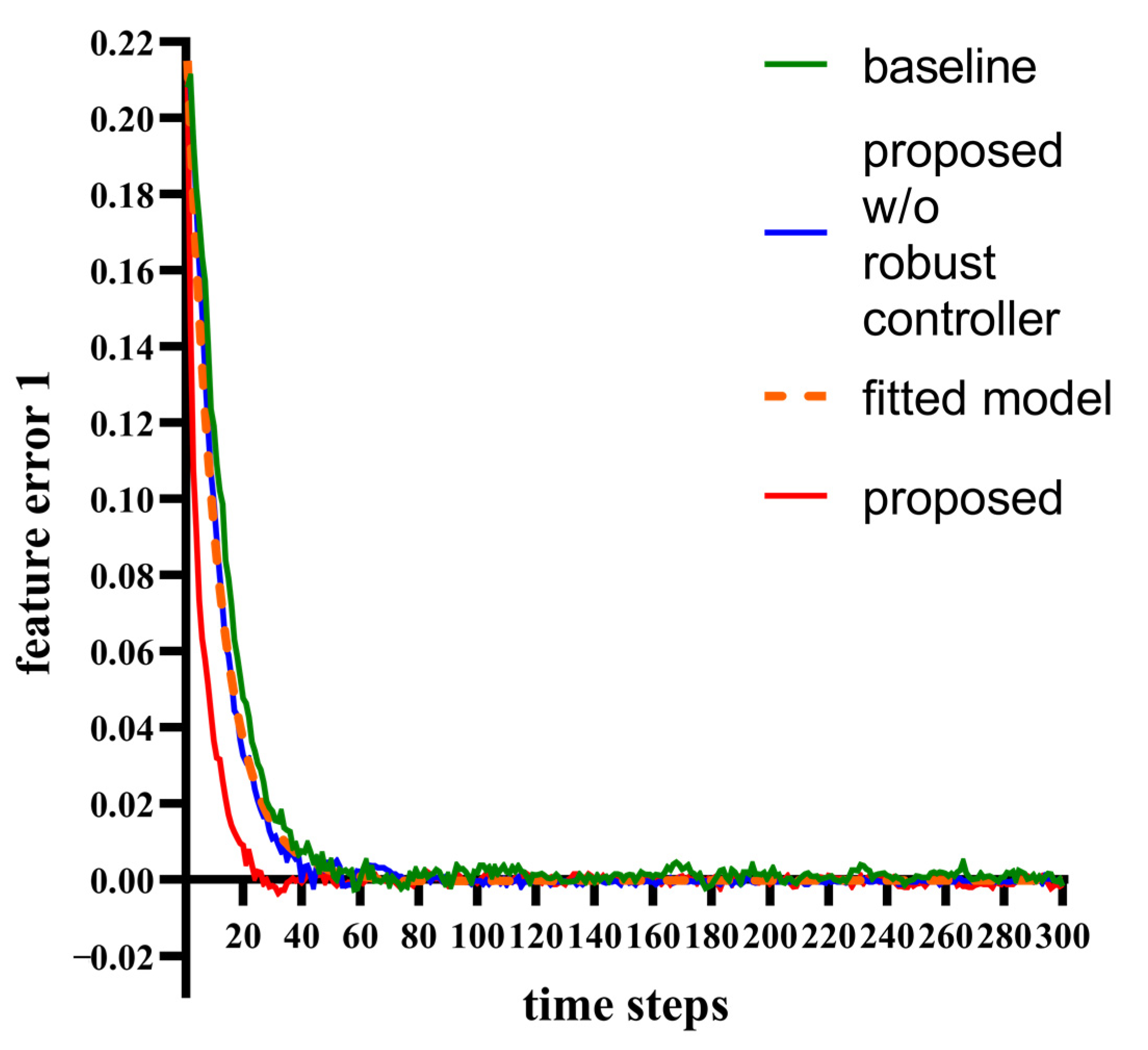
4.1. Ablation Study
4.2. Robustness to Noise
4.3. Adaptability to Fewer Samples
5. Conclusions
Author Contributions
Funding
Data Availability Statement
Conflicts of Interest
References
- Chopra, R.; Preston, G.C.; Keenan, T.D.L.; Mulholland, P.; Patel, P.J.; Balaskas, K.; Hamilton, R.D.; Keane, P.A. Intravitreal injections: Past trends and future projections within a UK tertiary hospital. Eye 2021, 36, 1373–1378. [Google Scholar] [CrossRef] [PubMed]
- Avery, R.L.; Bakri, S.J.; Blumenkranz, M.S.; Brucker, A.J.; Cunningham, E.T., Jr.; D’amico, D.J.; Dugel, P.U.; Flynn, H.W., Jr.; Freund, K.B.; Haller, J.A.; et al. Intravitreal Injection Technique And Monitoring: Updated Guidelines of an Expert Panel. Retina 2014, 34, S1–S18. [Google Scholar] [CrossRef] [PubMed]
- Campbell, R.J.; Bronskill, S.E.; Bell, C.M.; Paterson, J.M.; Whitehead, M.; Gill, S.S. Rapid Expansion of Intravitreal Drug Injection Procedures, 2000 to 2008 A Population-Based Analysis. Arch. Ophthalmol. 2010, 128, 359–362. [Google Scholar] [CrossRef] [PubMed] [Green Version]
- Agarwal, A.; Nagpal, M. Intravitreal moxifloxacin injections in acute post-cataract surgery endophthalmitis: Efficacy and safety. Indian J. Ophthalmol. 2021, 69, 326–330. [Google Scholar] [CrossRef]
- Roblain, Q.; Louis, T.; Yip, C.; Baudin, L.; Struman, I.; Caolo, V.; Lambert, V.; Lecomte, J.; Noël, A.; Heymans, S. Intravitreal injection of anti-miRs against miR-142-3p reduces angiogenesis and microglia activation in a mouse model of laser-induced choroidal neovascularization. Aging 2021, 13, 12359–12377. [Google Scholar] [CrossRef]
- DeSouza, P.; Nidamarthi, D.; Moshiri, A.; Yiu, G.; Park, S.S.; Emami-Naeini, P. Effect of intravitreal steroid injection or implant on visual and imaging outcomes in patients with non-infectious uveitis. Investig. Ophthalmol. Vis. Sci. 2021, 62, 732. [Google Scholar]
- Januschowski, K.; Boden, K.T.; Szurman, P.; Stalmans, P.; Siegel, R.; Pérez Guerra, N.; Becker, S.L.; Rickmann, A.; Bisorca-Gassendorf, L. Effectiveness of immediate vitrectomy and intravitreal antibiotics for post-injection endophthalmitis. Graefes Arch. Clin. Exp. Ophthalmol. 2021, 259, 1609–1615. [Google Scholar] [CrossRef]
- Scott, I.U.; Luu, K.M.; Davis, J.L. Intravitreal antivirals in the management of patients with acquired immunodeficiency syndrome with progressive outer retinal necrosis. Arch. Ophthalmol. 2002, 120, 1219–1222. [Google Scholar]
- Zhuang, H.; Ding, X.; Zhang, T.; Chang, Q.; Xu, G. Vitrectomy combined with intravitreal antifungal therapy for posttraumatic fungal endophthalmitis in eastern China. BMC Ophthalmol. 2020, 20, 435. [Google Scholar] [CrossRef]
- Cox, J.; Eliott, D.; Sobrin, L. Inflammatory Complications of Intravitreal Anti-VEGF Injections. J. Clin. Med. 2021, 10, 981. [Google Scholar] [CrossRef]
- Heimann, H. Intravitreal Injections: Techniques and Sequelae. In Medical Retina; Holz, F.G., Spaide, R.F., Eds.; Springer: Berlin/Heidelberg, Germany, 2007; pp. 67–87. [Google Scholar]
- Jalil, A.; Chaudhry, N.L.; Gandhi, J.S.; Odat, T.M.; Yodaiken, M. Inadvertent injection of triamcinolone into the crystalline lens. Eye 2007, 21, 152–154. [Google Scholar] [CrossRef] [PubMed] [Green Version]
- Han, J.; Davids, J.; Ashrafian, H.; Darzi, A.; Elson, D.S.; Sodergren, M. A systematic review of robotic surgery: From supervised paradigms to fully autonomous robotic approaches. Int. J. Med. Robot. Comput. Assist. Surg. 2021, 18, e2358. [Google Scholar] [CrossRef] [PubMed]
- Kisinde, S.; Hu, X.B.; Hesselbacher, S.; Lieberman, I.H. The predictive accuracy of surgical planning using pre-op planning software and a robotic guidance system. Eur. Spine J. 2021, 30, 3676–3687. [Google Scholar] [CrossRef] [PubMed]
- Topsakal, V.; Matulic, M.; Assadi, M.Z.; Mertens, G.; Van Rompaey, V.; Van de Heyning, P. Comparison of the Surgical Techniques and Robotic Techniques for Cochlear Implantation in Terms of the Trajectories Toward the Inner Ear. J. Int. Adv. Otol. 2020, 16, 3–7. [Google Scholar] [CrossRef]
- Sauvée, M.; Poignet, P.; Dombre, E. Ultrasound image-based visual servoing of a surgical instrument through nonlinear model predictive control. Int. J. Robot. Res. 2008, 27, 25–40. [Google Scholar] [CrossRef]
- Li, Q.; Du, Z.; Yu, H. Grinding trajectory generator in robot-assisted laminectomy surgery. Int. J. Comput. Assist. Radiol. Surg. 2021, 16, 485–494. [Google Scholar] [CrossRef]
- Cornella, K.N.; Palafox, B.A.; Razavi, M.K.; Loh, C.T.; Markle, K.M.; Openshaw, L.E. SAVI SCOUT as a Novel Localization and Surgical Navigation System for More Accurate Localization and Resection of Pulmonary Nodules. Surg. Innov. 2019, 26, 469–472. [Google Scholar] [CrossRef]
- Braun, D.; Yang, S.; Martel, J.N.; Riviere, C.N.; Becker, B.C. EyeSLAM: Real-time simultaneous localization and mapping of retinal vessels during intraocular microsurgery. Int. J. Med. Robot. Comput. Assist. Surg. 2018, 14, e1848. [Google Scholar] [CrossRef]
- Yang, S.; Martel, J.N.; Lobes, L.A.; Riviere, C.N. Techniques for robot-aided intraocular surgery using monocular vision. Int. J. Robot. Res. 2018, 37, 931–952. [Google Scholar] [CrossRef]
- Becker, B.C.; MacLachlan, R.A.; Lobes, L.A.; Hager, G.D.; Riviere, C.N. Vision-Based Control of a Handheld Surgical Micromanipulator With Virtual Fixtures. IEEE Trans. Robot. 2013, 29, 674–683. [Google Scholar] [CrossRef] [Green Version]
- Hutchinson, S.; Hager, G.D.; Corke, P.I. A tutorial on visual servo control. IEEE Trans. Robot. Autom. 1996, 12, 651–670. [Google Scholar] [CrossRef] [Green Version]
- Allen, M.; Westcoat, E.; Mears, L. Optimal Path Planning for Image Based Visual Servoing. Procedia Manuf. 2019, 39, 325–333. [Google Scholar] [CrossRef]
- Dilley, J.; Camara, M.; Omar, I.; Carter, A.; Pratt, P.; Vale, J.; Darzi, A.; Mayer, E.K. Evaluating the impact of image guidance in the surgical setting: A systematic review. Surg. Endosc. 2019, 33, 2785–2793. [Google Scholar] [CrossRef] [PubMed] [Green Version]
- Anderson, P.; Wu, Q.; Teney, D.; Bruce, J.; Johnson, M.; Sünderhauf, N.; Reid, I.; Gould, S.; van den Hengel, A. Vision-and-Language Navigation: Interpreting visually-grounded navigation instructions in real environments. In Proceedings of the 2018 IEEE/CVF Conference on Computer Vision and Pattern Recognition (CVPR), Salt Lake City, UT, USA, 18–22 June 2018. [Google Scholar]
- Mei, H.; Yang, X.; Wang, Y.; Liu, Y.; Lau, R. Don’t Hit Me! Glass Detection in Real-World Scenes. In Proceedings of the 2020 IEEE/CVF Conference on Computer Vision and Pattern Recognition (CVPR), Seattle, WA, USA, 14–19 June 2020. [Google Scholar]
- Molnár, C.; Nagy, T.D.; Elek, R.N.; Haidegger, T. Visual servoing-based camera control for the da Vinci Surgical System. In Proceedings of the 2020 IEEE 18th International Symposium on Intelligent Systems and Informatics (SISY), Subotica, Serbia, 17–19 September 2020; pp. 107–112. [Google Scholar]
- Hynes, P.; Dodds, G.I.; Wilkinson, A.J. Uncalibrated visual-servoing of a dual-arm robot for surgical tasks. In Proceedings of the 2005 International Symposium on Computational Intelligence in Robotics and Automation, Espoo, Finland, 27–30 June 2005; pp. 151–156. [Google Scholar]
- Ullrich, F.; Michels, S.; Lehmann, D.; Roel, S.P.; Becker, M.; Bradley, J.N. Assistive Device for Efficient Intravitreal Injections. Ophthalmic Surg. Lasers Imaging Retin. 2016, 47, 752–762. [Google Scholar] [CrossRef] [Green Version]
- Haidegger, T. Autonomy for Surgical Robots: Concepts and Paradigms. IEEE Trans. Med. Robot. Bionics 2019, 1, 65–76. [Google Scholar] [CrossRef]
- Yang, G.-Z.; Cambias, J.; Cleary, K.; Daimler, E.; Drake, J.; Dupont, P.E.; Hata, N.; Kazanzides, P.; Martel, S.; Patel, R.V.; et al. Medical robotics—Regulatory, ethical, and legal considerations for increasing levels of autonomy. Sci. Robot. 2017, 2, eaam8638. [Google Scholar] [CrossRef]
- Maillard, E.P.; Gueriot, D. Ieee, RBF neural network, basis functions and genetic algorithm. In Proceedings of the 1997 IEEE International Conference on Neural Networks, Houston, TX, USA, 12 June 1997; Volume 1–4. [Google Scholar]
- Fedorenko, F.; Usilin, S. Real-time object-to-features vectorisation via Siamese neural networks. In Proceedings of Ninth International Conference on Machine Vision (ICMV 2016), Nice, France, 18–20 November 2016. [Google Scholar]
- Hajiloo, A.; Keshmiri, M.; Xie, W.-F.; Wang, T.-T. Robust On-Line Model Predictive Control for a Constrained Image Based Visual Servoing. IEEE Trans. Ind. Electron. 2015, 63, 2242–2250. [Google Scholar] [CrossRef]
- Zhang, J.; Liu, D. Online Estimation of Image Jacobian Matrix Based on Robust Information Filter. J. Xi’an Univ. Technol. 2011, 27, 133–138. [Google Scholar]
- Corke, P. Vision-Based Control. In Robotics, Vision and Control: Fundamental Algorithms in MATLAB®; Corke, P., Ed.; Springer: Berlin/Heidelberg, Germany, 2011; pp. 455–479. [Google Scholar]
- Fazekas, Z.; Lócsi, L.; Soumelidis, A.; Schipp, F.; Németh, Z. Rational Zernike Functions Capture the Rotations of the Eye-Ball. In Progress in Industrial Mathematics at ECMI 2018; Springer International Publishing: Cham, Switzerland, 2019; pp. 215–221. [Google Scholar] [CrossRef]
- Poonguzhal, N.; Ezhilarasa, M. Identification Based on Iris Geometric Features. J. Appl. Sci. 2015, 15, 792–799. [Google Scholar] [CrossRef] [Green Version]
- Masek, L. Recognition of Human Iris Patterns for Biometric Identification. Master’s Thesis, University of Western Australia, Crawley, WA, Australia, 2003. [Google Scholar]
- Pierce, J.E.; Clementz, B.A.; McDowell, J.E. Saccades: Fundamentals and Neural Mechanisms. In Eye Movement Research: An Introduction to Its Scientific Foundations and Applications; Klein, C., Ettinger, U., Eds.; Springer International Publishing: Cham, Switzerland, 2019; pp. 11–71. [Google Scholar]
- Green-Simms, A.E.; Ekdawi, N.S.; Bakri, S.J. Survey of Intravitreal Injection Techniques Among Retinal Specialists in the United States. Am. J. Ophthalmol. 2011, 151, 329–332. [Google Scholar] [CrossRef]
- Haeussler-Sinangin, Y.; Kohnen, T. Corneal Diameter. In Encyclopedia of Ophthalmology; Schmidt-Erfurth, U., Kohnen, T., Eds.; Springer: Berlin/Heidelberg, Germany, 2018; pp. 521–522. [Google Scholar]
- Colan, J.; Nakanishi, J.; Aoyama, T.; Hasegawa, Y. Optimization-Based Constrained Trajectory Generation for Robot-Assisted Stitching in Endonasal Surgery. Robotics 2021, 10, 27. [Google Scholar] [CrossRef]
- Zouaoui, R.; Mekki, H. 2D visual servoing of wheeled mobile robot by neural networs. In Proceedings of the 2013 International Conference on Individual and Collective Behaviors in Robotics (ICBR), Sousse, Tunisia, 15–17 December 2013; pp. 130–133. [Google Scholar]
- Wang, F.; Sun, F.; Zhang, J.; Lin, B.; Li, X. Unscented Particle Filter for Online Total Image Jacobian Matrix Estimation in Robot Visual Servoing. IEEE Access 2019, 7, 92020–92029. [Google Scholar] [CrossRef]
- Salehian, M.; RayatDoost, S.; Taghirad, H.D. Robust unscented Kalman filter for visual servoing system. In Proceedings of the 2nd International Conference on Control, Instrumentation and Automation, Shiraz, Iran, 27–29 December 2011. [Google Scholar] [CrossRef]
- Ren, X.; Li, H.; Li, Y. Online Image Jacobian Identification Using Optimal Adaptive Robust Kalman Filter for Uncalibrated Visual Servoing. In Proceedings of the 2017 2ND Asia-Pacific Conference on Intelligent Robot Systems (ACIRS), Wuhan, China, 16–18 June 2017. [Google Scholar]
- Zhao, Q.; Zhang, L.; Chen, Y. Online estimation technique for Jacobian matrix in robot visual servo systems. In Proceedings of the 2008 3rd IEEE Conference on Industrial Electronics and Applications, Singapore, 3–5 June 2008; pp. 1270–1275. [Google Scholar]
- Zhang, Y.-B. Unscented Kalman filter for on-line estimation of Jacobian matrix. J. Comput. Appl. 2011, 31, 1699–1702. [Google Scholar] [CrossRef]
- Qian, J.; Su, J. Online estimation of image Jacobian matrix by Kalman-Bucy filter for uncalibrated stereo vision feedback. In Proceedings of the 2002 IEEE International Conference on Robotics and Automation (Cat. No. 02CH37292), Washington, DC, USA, 11–15 May 2002; Volume 1, pp. 562–567. [Google Scholar]
- Gu, J.; Wang, H.; Pan, Y.; Wu, Q. Neural network based visual servo control for CNC load/unload manipulator. Optik 2015, 126, 4489–4492. [Google Scholar] [CrossRef]
- Matter, E. Epipolar-kinematics relations estimation neural approximation for robotics closed loop visual servo system. In Proceedings of the 2010 2nd International Conference on Computer and Automation Engineering (ICCAE 2010), Singapore, 26–28 February 2010; Volume 5, pp. 441–445. [Google Scholar] [CrossRef]
- Nakamura, Y.; Hanafusa, H. Inverse Kinematic Solutions With Singularity Robustness for Robot Manipulator Control. J. Dyn. Syst. Meas. Control 1986, 108, 163–171. [Google Scholar] [CrossRef]
- Halír, R.; Flusser, J. Numerically stable direct least squares fitting of ellipses. In Proceedings of the 6th International Conference in Central Europe on Computer Graphics and Visualization, WSCG, Bory, Czech Republic, 9–13 February 1998; Volume 98, pp. 125–132. [Google Scholar]
- Wang, F.; Liu, Z.; Chen, C.; Zhang, Y. Adaptive neural network-based visual servoing control for manipulator with unknown output nonlinearities. Inf. Sci. 2018, 451–452, 16–33. [Google Scholar] [CrossRef]
- Loreto, G.; Yu, W.; Garrido, R. Stable visual servoing with neural network compensation. In Proceedings of the 2001 IEEE International Symposium on Intelligent Control (ISIC’01), Mexico City, Mexico, 5–7 September 2001; pp. 183–188. [Google Scholar]
- Qiu, Z.; Wu, Z. Adaptive neural network control for image-based visual servoing of robot manipulators. IET Control Theory Appl. 2022, 16, 443–453. [Google Scholar] [CrossRef]
- Chicco, D. Siamese Neural Networks: An Overview. In Artificial Neural Networks. Methods in Molecular Biology; Cartwright, H., Ed.; Springer: New York, NY, USA, 2020; Volume 2190, pp. 73–94. [Google Scholar]
- Tokuda, F.; Arai, S.; Kosuge, K. Convolutional Neural Network-Based Visual Servoing for Eye-to-Hand Manipulator. IEEE Access 2021, 9, 91820–91835. [Google Scholar] [CrossRef]
- Hemingway, E.G.; O’Reilly, O.M. Perspectives on Euler angle singularities, gimbal lock, and the orthogonality of applied forces and applied moments. Multibody Syst. Dyn. 2018, 44, 31–56. [Google Scholar] [CrossRef]
- Hendrycks, D.; Gimpel, K. Gaussian error linear units (gelus). arXiv 2016, arXiv:1606.08415. [Google Scholar]
- Park, F.C.; Bobrow, J.E.; Ploen, S.R. A lie group formulation of robot dynamics. Int. J. Robot. Res. 1995, 14, 609–618. [Google Scholar] [CrossRef]
- Zhuang, J.; Tang, T.; Ding, Y.; Tatikonda, S.C.; Dvornek, N.; Papademetris, X.; Duncan, J. Adabelief optimizer: Adapting stepsizes by the belief in observed gradients. Adv. Neural Inf. Process. Syst. 2020, 33, 18795–18806. [Google Scholar]
- Paszke, A.; Gross, S.; Massa, F.; Lerer, A.; Bradbury, J.; Chanan, G.; Killeen, T.; Lin, Z.; Gimelshein, N.; Antiga, L.; et al. Pytorch: An imperative style, high-performance deep learning library. Adv. Neural Inf. Process. Syst. 2019, 32, 8026–8037. [Google Scholar]
- Bartoszewicz, A. Discrete-time quasi-sliding-mode control strategies. IEEE Trans. Ind. Electron. 1998, 45, 633–637. [Google Scholar] [CrossRef]
- Rohmer, E.; Singh, S.P.N.; Freese, M. V-REP: A versatile and scalable robot simulation framework. In Proceedings of the 2013 IEEE/RSJ International Conference on Intelligent Robots and Systems, Tokyo, Japan, 3–7 November 2013; pp. 1321–1326. [Google Scholar]
- Sarker, A.; Sinha, A.; Chakraborty, N. On Screw Linear Interpolation for Point-to-Point Path Planning. In Proceedings of the 2020 IEEE/RSJ International Conference on Intelligent Robots and Systems (IROS), Las Vegas, NV, USA, 25–29 October 2020; pp. 9480–9487. [Google Scholar]
- Fabisch, A. pytransform3d: 3D Transformations for Python. J. Open Source Softw. 2019, 4, 1159. [Google Scholar] [CrossRef]
- Maxim, A.; Lazar, C.; Burlacu, A.; Copot, C. Robotic visual servoing system based on SIFT features. In Proceedings of the 2012 16th International Conference on System Theory, Control and Computing (ICSTCC 2012), Sinaia, Romania, 12–14 October 2012; pp. 1–6. [Google Scholar]
- Assa, A.; Janabi-Sharifi, F. Two DOF controller for decoupled image-based visual servoing. In Proceedings of the 2014 IEEE 27th Canadian Conference on Electrical and Computer Engineering (CCECE), Toronto, ON, Canada, 4–7 May 2014; pp. 1–6. [Google Scholar]
- Reghenzani, F.; Massari, G.; Fornaciari, W. The Real-Time Linux Kernel: A Survey on PREEMPT_RT. ACM Comput. Surv. 2019, 52, 18. [Google Scholar] [CrossRef]


| Item | Baseline | Proposed |
|---|---|---|
| Rise steps | 28 | 14 |
| Overshoot | 1.23% | 1.62% |
| Standard deviation of balance position | 1.09 × 10⁻³ | 9.48 × 10⁻⁴ |
| Simulation test final translation error (mm) | 5.1 | 0.5 |
| Simulation test final rotation error (rad) | 0.0607 | 0.0438 |
| Distance between injection site and iris edge (mm) | 1.31 | 3.68 |
| Angle of injection point deviation from horizontal line (rad) | 0.0937 | 0.2391 |
| Proposed | w/o Robust Controller | w/o GELU | w/o Proposed Loss | |
|---|---|---|---|---|
| Rise steps | 14 | 25 | 5 | 6 |
| Overshoot | 1.62% | 0.20% | 2.04% | 1.32% |
| Simulation test final translation error (mm) | 0.5 | 0.7 | 1.6 | 0.8 |
| Simulation test final rotation error (rad) | 0.0438 | 0.0485 | 0.0407 | 0.0419 |
| Distance between injection site and iris edge (mm), reference value: 3.5 | 3.68 | 3.55 | 4.03 | 3.45 |
| Angle of injection point deviation from horizontal line (rad) | 0.2391 | 0.241 | 0.195 | 0.240 |
| SNR | ∞ | 100 dB | 80 dB | 60 dB | 50 dB | 45 dB |
|---|---|---|---|---|---|---|
| Translation error (mm) | 0.7 | 0.7 | 0.7 | 0.7 | 0.6 | 0.8 |
| Rotation error (rad) | 0.0485 | 0.0486 | 0.0486 | 0.0488 | 0.0489 | 0.0421 |
| Distance between injection site and iris edge (mm) | 3.55 | 3.55 | 3.55 | 3.53 | 3.54 | 3.98 |
| Angle of injection point deviation from horizontal line (rad) | 0.241 | 0.241 | 0.241 | 0.241 | 0.245 | 0.235 |
| Sampling Rate | 100% | 75% | 50% | 25% | 10% |
|---|---|---|---|---|---|
| Translation error (mm) | 0.7 | 0.7 | 0.8 | 0.9 | 1.1 |
| Rotation error (rad) | 0.0485 | 0.0490 | 0.0481 | 0.0480 | 0.0437 |
| Distance between injection site and iris edge (mm) | 3.55 | 3.57 | 3.57 | 3.77 | 4.12 |
| Angle of injection point deviation from horizontal line (rad) | 0.241 | 0.228 | 0.247 | 0.243 | 0.188 |
Publisher’s Note: MDPI stays neutral with regard to jurisdictional claims in published maps and institutional affiliations. |
© 2022 by the authors. Licensee MDPI, Basel, Switzerland. This article is an open access article distributed under the terms and conditions of the Creative Commons Attribution (CC BY) license (https://creativecommons.org/licenses/by/4.0/).
Share and Cite
He, X.; Luo, H.; Feng, Y.; Wu, X.; Diao, Y. An Uncalibrated Image-Based Visual Servo Strategy for Robust Navigation in Autonomous Intravitreal Injection. Electronics 2022, 11, 4184. https://doi.org/10.3390/electronics11244184
He X, Luo H, Feng Y, Wu X, Diao Y. An Uncalibrated Image-Based Visual Servo Strategy for Robust Navigation in Autonomous Intravitreal Injection. Electronics. 2022; 11(24):4184. https://doi.org/10.3390/electronics11244184
Chicago/Turabian StyleHe, Xiangdong, Hua Luo, Yuliang Feng, Xiaodong Wu, and Yan Diao. 2022. "An Uncalibrated Image-Based Visual Servo Strategy for Robust Navigation in Autonomous Intravitreal Injection" Electronics 11, no. 24: 4184. https://doi.org/10.3390/electronics11244184