Gaussian Mixture with Max Expectation Guide for Stacked Architecture of Denoising Autoencoder and DRBM for Medical Chest Scans and Disease Identification

Abstract

Artificial intelligence (AI), in particular deep learning, has proven to be efficient in medical diagnosis. This paper introduces a new hybrid deep learning model for pneumonia diagnosis based on chest CT scans. At the core of the model, a Gaussian mixture is combined with the expectation-maximization algorithm (EMGMM) to extract the regions of interest (ROI), while a convolutional denoising autoencoder (DAE) and deep restricted Boltzmann machine (DRBM) are combined for the classification. In order to prevent the model from learning trivial solutions, stochastic noises were added as an input to the unsupervised learning phase. The dataset used in this work is a publicly available dataset of chest X-rays for pneumonia on the Kaggle website; it contains 5856 images with 1583 normal cases and 4273 pneumonia cases, with an imbalance ratio (IR) of 0.46. Several operations including zooming, flipping, shifting and rotation were used in the augmentation phase to balance the data distribution across the different classes, which led to enhancing the IR value to 0.028. The computational analysis of the results show that the proposed model is promising as it provides an average accuracy value of 98.63%, sensitivity value of 96.5%, and specificity value of 94.8%.

1. Introduction

Medical images such as MRI or X-ray scans allow for a better diagnosis process without the need for surgery. Chest X-ray (CXR), for example, is considered an important requirement to diagnose the COVID-19 virus. Recently, integrating AI techniques in medical scan machines has improved the detection of infected parts and has aided in the diagnosis process. One of the serious diseases that infect the lungs and cause respiratory system defects is pneumonia, which can be caused by different types of viruses, bacteria, fungi, or chemical exposure [1]. It dangerously fills the lungs with fluids and minimizes the carbon dioxide exhalation causing breath struggle, fainting, fever, and other symptoms that may lead to sudden death based on the severity and intensity of the infection [2]. Accordingly, the early detection of pneumonia is a very important step in order to prevent patients from having severe symptoms, save them from disorder complications [3], and treat them with low-cost medications.

Various AI techniques have been used in automatic analysis systems for noninvasive pneumonia detection and diagnosis, which has led to quicker, more accurate, and more reliable treatment decisions [4,5]. Recently, deep learning has shown better performance over traditional AI techniques for medical image classification [6,7,8]. Although deep learning models [9,10,11] have allowed for fast and accurate diagnosis, the efficiency and effectiveness of these models have mainly relied on their hyperparameter values.Choosingsuitable hyperparameter values is a critical task in order to create an efficient model for the problem at hand. Several models have achieved high accuracies, especially when they combine supervised and unsupervised learning, such as deep restricted Boltzmann machine (DRBM) [12,13,14], convolution neural network (CNN) [7,8], and denoising autoencoder [15,16].

This paper introduces a new hybrid deep learning model that at its core uses the EMGMM as a guide for a multi-phased model to improve the total training time and complexity. The model also integrates the DAE and DRBM to assist with the prediction of chest diseases. The EMGMM allows for the efficient extraction of the ROI, while the DAE prevents the model from learning trivial representations during the feature extraction phase from healthy and unhealthy (pneumonia) cases. Finally, the DRBM provides an extra layer that aims to extract the abstract features and increases the robustness and generalization to avoid over-fitting.

The main contributions of this work can be summarized as follows: (1) the ability of the model to extract the ROI based on the EMGMM that combines both the Gaussian mixture and the Max Expectation segmentation with thresholding boundary detection; (2) the use of a hybrid model that combines DAE and DRBM for better generalization and robustness; (3) the ability of the proposed model to achieve higher accuracy rate over existing works when applied to the same large CT scans dataset.

The paper is structured as follows: Section 2 focuses on similar research in the literature that used deep-learning models to diagnose chest diseases based on CXR. Section 3 introduces the proposed model and its constituents. Section 4 presents the experimental setup and discussion of results, in addition to a comparison between the proposed model’s performance and similar studies. Finally, Section 5 concludes this work.

2. Literature Review

Pneumonia, one of the most common chest diseases, can be diagnosed by radiologists using CXRs. Several AI techniques [17,18,19] and analytical models [20,21] have been devoted to diagnosing pneumonia from lung X-ray images. Deep learning techniques were used for image analysis and diagnosis-based classification [7,8,9,10,11,12] showing significant performance in identifying infected regions with high accuracy. The remainder of this section surveys existing deep-learning models that aimed to diagnose chest diseases based on CXR.

In [15], the authors built a deep learning model for automatic COVID-19 detection based on CT scans using four convolution layers trained by the autoencoder. Each layer of the stacked autoencoder detector was separately trained to guarantee dimensionality reduction and better feature extraction. The authors reported that the model achieved 94.7% accuracy using 5-cross folding. This might be considered not to be a high enough accuracy based on the fact that the model was trained on a small dataset of CT scans with 470 cases only.

In [22], the authors built a CNN deep-learning model to detect different types of pneumonia including COVID-19. Firstly, they used meta-learner optimization by training the model using either normal or non-COVID-pneumonia cases. Then, they utilized depth-wise convolution with several dilation rates to extract optimal diversified features from chest X-rays of pneumonia. High accuracy of 98.1% was achieved while detecting normal versus pneumonia cases, and moderate accuracy of 90.2% for COVID-19/Viral pneumonia classification.

In [23], researchers constructed a deep CNN to diagnose pneumonia disease. Their architecture utilizes backpropagation neural networks (BPNNs) for error enhancement and competitive neural networks (CpNNs) to allow for both supervised and unsupervised learning opportunities. They concluded that CNN has better generalization power than that achieved by BPNN, whereas it suffers from high computational time and a large number of iterations. The model achieved an accuracy of 92.4% using CNN, and a minimum and maximum accuracy of 80.04% and 92% respectively when applying the BPNNs and CpNNs models.

In [24], the authors introduced a CNN model to detect pneumonia from 5856 x-ray chest scans for children from 1–5 years old. The authors used data augmentation algorithms to improve the classification power of the model. The model achieved an accuracy of 95.31% when applied to 200 data samples in the training phase and 93.73% in the validation phase, which are good results but not high enough.

In [25], the authors used an ensemble of three convolution neural network models: GoogLeNet, ResNet-18, and DenseNet-121 to detect pneumonia disease. Their proposed model was developed using two different chest x-ray images: Kermany and RSNA. Although the ensemble model achieved an accuracy of 98.81% for the Kermany dataset, and 86.85% for RSNA, the imbalance ratio for the Kermany dataset was 0.46, which might have played a role in the resulting high accuracy, especially in view of the small number of healthy, or normal, patients. Regrettably, this issue was not addressed by the authors in their work.

In [26], the authors used a CSAC-Net deep-learning model to diagnose mild COVID-19 pneumonia. The dataset included 2087 chest CT exams collected from four hospitals. The overall sensitivity was 91.5%, the specificity was 90.5%, and the general AUC value was 95.5%. The proposed deep learning model was trained on 1538 patients and tested on an independent testing cohort of 549 patients. Despite the small number fCT scans used in this work (AUC), the specificity and sensitivity values are not high enough and might even get lower with the use of a larger number of cases.

The authors in [27] detected pneumonia from chest scans by using a deep learning model. They constructed a convolutional sparse denoising autoencoder to minimize the reconstruction error and to obtain the set of features. They applied a voting scheme to identify the case as normal or infected and evaluated their model on four publicly available radiology datasets of chest scans. Despite thousands of CT scans used in the training phase, the achieved average accuracy for both normal and abnormal classes was 96.5% with a precision of 97.9%, which is high but not as high as other models including the proposed model in this paper.

In [28], the authors were motivated by the increased cases of pneumonia and suspected infection with COVID-19. They proposed an efficient technique based on the DAE model, which provided a satisfying depiction of the CT scans in addition to successful extraction of the main features from a balanced dataset using augmentation. Their architecture contained 8-autoencoders, two dense layers, and a SoftMax layer for classification. The technique was applied to a dataset of 5856 images and an additional 125 images from another dataset: the achieved average accuracy was 96.8% with 93% precision and 92% recall. It is worth noting that this is the same dataset we adopted for our work.

The previous works used the DAE to extract the significant features and an additional SoftMax layer in their classifiers. Some others considered the autoencoder and the hidden features with a similar construction model. Instead, our model integrates EMGMM for ROI extraction and the hybrid DAE-DRBM in the classification task (which is a novel approach). The hybrid model uses the hidden features along with a cascade model with different roles of the DRBM for better generalization, and was able to achieve an average accuracy of 98.63% (the highest accuracy among all the surveyed models).

3. Background

This section presents the different techniques that were considered in the proposed model along with a brief description including the expectation-maximization technique, the Gaussian mixture model, the deep autoencoder model, and the deep restricted Boltzmann machine model (DRBM).

3.1. Expectation-Maximization Guided Gaussian Mixture Segmentation (EMGMM)

The Gaussian mixture model (GMM) allows for accurate image segmentation with precise region description and accurate categorization of these segments based on the image size and shape [27,28]. The images are represented as a set of pixels with values that reflect their intensity or color; assume (a) I = {i₁, i₂, …, i_n} is a stochastic random variable; w_{j =} j = 1, …, q are the corresponding weights satisfying ${\displaystyle \sum }_{\mathrm{j}=1}^{\mathrm{q}}{\mathrm{w}}_{\mathrm{j}}=1$, $\mathrm{n}\left(\mathrm{I}/{\varnothing }_{\mathrm{j}},{{{\displaystyle \sum }}^{\text{}}}_{\mathrm{j}}\right)$; and j = 1, …, q are the Gaussian densities; and (b) ${\varnothing }_{\mathrm{j}}$ is the mean vector while ${{{\displaystyle \sum }}^{\text{}}}_{\mathrm{j}}$ is the covariance matrix of the jth Gaussian. The GMMs maximize the probability of the parameters (e.g., means, covariance, and mixing coefficients). The multi-variant Gaussian mixture distribution can be defined by Equation (1):

$$\mathrm{mgd}\left(\mathrm{I}\right)={\displaystyle \sum }_{\mathrm{j}=1}^{\mathrm{k}}{\mathrm{w}}_{\mathrm{j}}\mathrm{n}\left(\mathrm{I}/{\varnothing }_{\mathrm{j}},{{{\displaystyle \sum }}^{\text{}}}_{\mathrm{j}}\right),\mathrm{n}(\mathrm{I}/{\varnothing }_{\mathrm{j}},{{{\displaystyle \sum }}^{\text{}}}_{\mathrm{j}})=\frac{1}{\sqrt{{\left(2\mathsf{\pi }\right)}^2\left|{{{\displaystyle \sum }}^{\text{}}}_{\mathrm{j}}\right|}}\exp \left[-\frac{1}{2}{\left(\mathrm{I}-{\varnothing }_{\mathrm{j}}\right)}^{\mathrm{T}}{\displaystyle \sum }_{\mathrm{j}}^{}\left(\mathrm{I}-{\varnothing }_{\mathrm{j}}\right)\right].$$

(1)

The GMM algorithm selects pre-defined clusters (k) at the beginning based on the sample distribution. However, in image segmentation, it is absolutely necessary to estimate the best value of the GMM parameters. The (EM) algorithm targets the optimal GMM parameters. Hence, the segments of the image can be efficiently obtained. In fact, the GMM mixture models calculate the maximum likelihood probability for each pixel color’sbelonging to a particular segment. The algorithm is a continuous optimization approach that iteratively attempts to obtain the parameters of each segment [29,30]. The parameters of ${\varnothing }_{\mathrm{j}}$ and ${{{\displaystyle \sum }}^{\text{}}}_{\mathrm{j}}$ for each cluster act as an input to the EM algorithm. The algorithm stops in one of the following cases: (1) the estimations of the new objective parameters’ values reach the defined value; or (2) the predefined number of iterations is reached.

The maximum value of the algorithm is computed over two steps (E-step and M-step): E-step evaluates the responsibilities of the latent variable for given parameter values, while the maximization step (M-step) maximizes the parameters and updates them with new values. More information about these steps are provided below:

• E-Step: suppose the parameter value is ${\varnothing }_{\mathrm{j}}$, calculate ${\displaystyle \sum }_{\mathrm{j}=1}^{\mathrm{k}}{\mathrm{w}}_{\mathrm{j}}=1\mathrm{for}$ all data points Ij, 1 ≤ j ≤ n and all mixture components 1 ≤ k ≤ K, which yields an n × K membership weights matrix.
• M-Step: in this step, the maximization of the parameters is reached based on the previous matrix. Let n = count of the membership weights, such that ${\displaystyle \sum }_{\mathrm{j}=1}^{\mathrm{k}}{\mathrm{w}}_{\mathrm{j}}=1$ is the sum of the membership weights for the kth parameter; as seen in Equation (2), the values of weights and means are then updated respectively:

  $${\mathsf{\mu }}_{\mathrm{k}}^{\mathrm{updated}}=\frac{{\mathrm{n}}_{\mathrm{k}}}{\mathrm{n}},1\le \mathrm{k}\le \mathrm{K},$$

  $${\mathsf{\mu }}_{\mathrm{k}}^{\mathrm{updated}}=\left(\frac{1}{{\mathrm{n}}_{\mathrm{k}}}\right){\displaystyle \sum }_{\mathrm{k}=1}^{\mathrm{K}}{\mathrm{w}}_{\mathrm{jk}}{\mathrm{I}}_{\mathrm{j}},1\le \mathrm{k}\le \mathrm{K},$$

  $${\mathsf{\mu }}_{\mathrm{k}}^{\mathrm{updated}}=\left(\frac{1}{n_{\mathrm{k}}}\right){\displaystyle \sum }_{\mathrm{k}=1}^{\mathrm{K}}{\mathrm{w}}_{\mathrm{jk}}\left({\mathrm{I}}_{\mathrm{j}}-{\varnothing }_{\mathrm{k}}^{\mathrm{updated}}{}_{}\right){\left({\mathrm{I}}_{\mathrm{j}}-{\varnothing }_{\mathrm{k}}^{\mathrm{updated}}{}_{}\right)}^{\mathrm{T}},1\le \mathrm{k}\le \mathrm{K}.$$

  (2)

3.2. Autoencoder (AE)

The autoencoder (AE) is a feed-forward neural network with 2L + 1 hidden layers. During training, the model aims to learn a compact and valuable representation based on the weight matrix, which will then act as an estimate of the input data and regenerate the look-up map pixels [31]. Assuming the autoencoder takes an input i with a defined representation DR in a certain domain d (i Є DR_d), it would work as follows:

(1) The encoder maps i to a lower dimensional representation (h Є R_d) by using a deterministic function h_l = f_l (i) = α(W_li + b_l), where α is the hyperbolic tangent activation function (W_l = weight matrix and b_l = bias term for encoder).

(2) The decoder acts as a mirror or reverse mapping for the output o by another deterministic function o = f_l (h) = α (W’_lh + b’_l) with l’ = lW’b (W’ = weight matrix and b’ = bias for the decoder).

(3) During the training phase, step (2) is repeated for each i (mapped to its abstraction h and new rebuild o) with an optimal cost function for fine-tuning.

The use of deep convolutional AE has provided tremendous promise for neuroimaging and medical scans [32]. Generally, each fully connected layer is replaced by several convolutional, pooling, and normalization layers, where the number of these layers depends on the problem at hand and the target performance. The mathematical formulas of the convolutional autoencoder are very similar to the elemental autoencoder stated earlier, except that the weights are shared. For input I, the representation of the jth feature map is stated in Equation (3), where b is distributed over the whole map, α is the activation function, and * means convolution:

h_j = α (i*W^j + b^j)

(3)

The produced input to the decoder is formulated as in Equation (4), where c = bias per one input channel, h = the feature maps, and W″ = the reverse operation of the weights mapping. The cost function (mean squared error) is shown in Equation (5) in which the backpropagation computes the gradient of the error, where d_h and d_o are the differences in the hidden and output layers, respectively. A stochastic gradient descent in Equation (6) modifies the weights, and the class label o″ is estimated by Equation (7).

$$\mathrm{o}=\mathrm{v}\left({{\displaystyle \sum }}_{\mathrm{j}\in \mathrm{H}}{\mathrm{h}}^{\mathrm{j}}{\ast \mathrm{W}}^{\text{”}\mathrm{j}}+\mathrm{c}\right)$$

(4)

$${\mathrm{e}}_{\propto }=\frac{1}{2\mathrm{n}}{{\displaystyle \sum }}_{\mathrm{i}=1}^{\mathrm{n}}{\left({\mathrm{i}}_{\mathrm{k}}-{\mathrm{o}}_{\mathrm{k}}\right)}^2$$

(5)

$$\frac{{\mathsf{\delta }\mathrm{e}}_{\mathsf{\alpha }}}{{\mathsf{\delta }\mathrm{W}}^{\mathrm{j}}}={\mathrm{i}\ast \mathrm{d}}_{{\mathrm{h}}^{\mathrm{j}}}+{\mathrm{h}}^{~\mathrm{j}}{\ast \mathrm{d}}_{\mathrm{o}}$$

(6)

$${\mathrm{o}}^{\text{”}}=\{\begin{array}{cc}1& \mathrm{if}\mathrm{k}\ge 0.5\\ 0& \mathrm{if}\mathrm{k}<0.5\end{array}$$

(7)

Additionally, the denoising autoencoder (DAE) [33] is a robust variant of the AE that accepts a stochastic noisy representation of the input by using the Gaussian additive noise while comparing it with the given ideal input, and hence reaching the optimal set of weights that highlight the discriminative features.

3.3. Deep Restricted Boltzmann Machine (DRBM)

Restricted Boltzmann Machine (RBM) [10,11,12,13,14] is considered a variant of Markov Random Field. It contains visible sophisticated variables sv = (sv₁, sv₂… sv_i) and arbitrary hidden variables rh = {rh₁, rh₂, rh_J}. It is bidirectional, between sv and rh, where both pivot on the major features. This constrains direct neurons to being allied to the bipartite model. Mathematically, the RBM is a probabilistic energy algorithm that aims to reach a probability distribution (pd) association graph of sv and rh as shown in Equations (8)–(10).

$$\mathrm{Pd}\left(\mathrm{sv}\right)=\frac{1}{\mathrm{i}}{\exp }^{-\mathrm{E}\left(\mathrm{sv}\right)},$$

(8)

$$\mathrm{Pd}\left(\mathrm{sv}\right)={\displaystyle \sum }_{\mathrm{hn}}\mathrm{Pd}\left(\mathrm{sv},\mathrm{rh}\right)={\displaystyle \sum }_{\mathrm{rh}}\frac{1}{\mathrm{i}}{\exp }^{-\mathrm{E}\left(\mathrm{sv},\mathrm{rh}\right)},$$

(9)

$$\mathrm{E}\left(\mathrm{sv},\mathrm{rh}\right)=-{{\displaystyle \sum }}_{\mathrm{ij}}\frac{1}{{\mathsf{\sigma }}_{\mathrm{i}}}{\mathrm{sv}}_{\mathrm{i}}{\mathrm{w}}_{\mathrm{ij}}{\mathrm{rh}}_{\mathrm{j}}-{{\displaystyle \sum }}_{\mathrm{i}}\frac{{\left({\mathrm{a}}_{\mathrm{i}}-{\mathrm{sv}}_{\mathrm{i}}\right)}^2}{{\mathsf{\sigma }}_{\mathrm{i}}^2}-{{\displaystyle \sum }}_{\mathrm{j}}{\mathrm{b}}_{\mathrm{j}}{\mathrm{h}}_{\mathrm{j}}$$

(10)

In the above equations, i is a normalized term; W_ij are weights sv_i→rh_j; (a_i, b_j) are biases for visible and hidden variables; and σ_i is the standard deviation for the Gaussian noise.

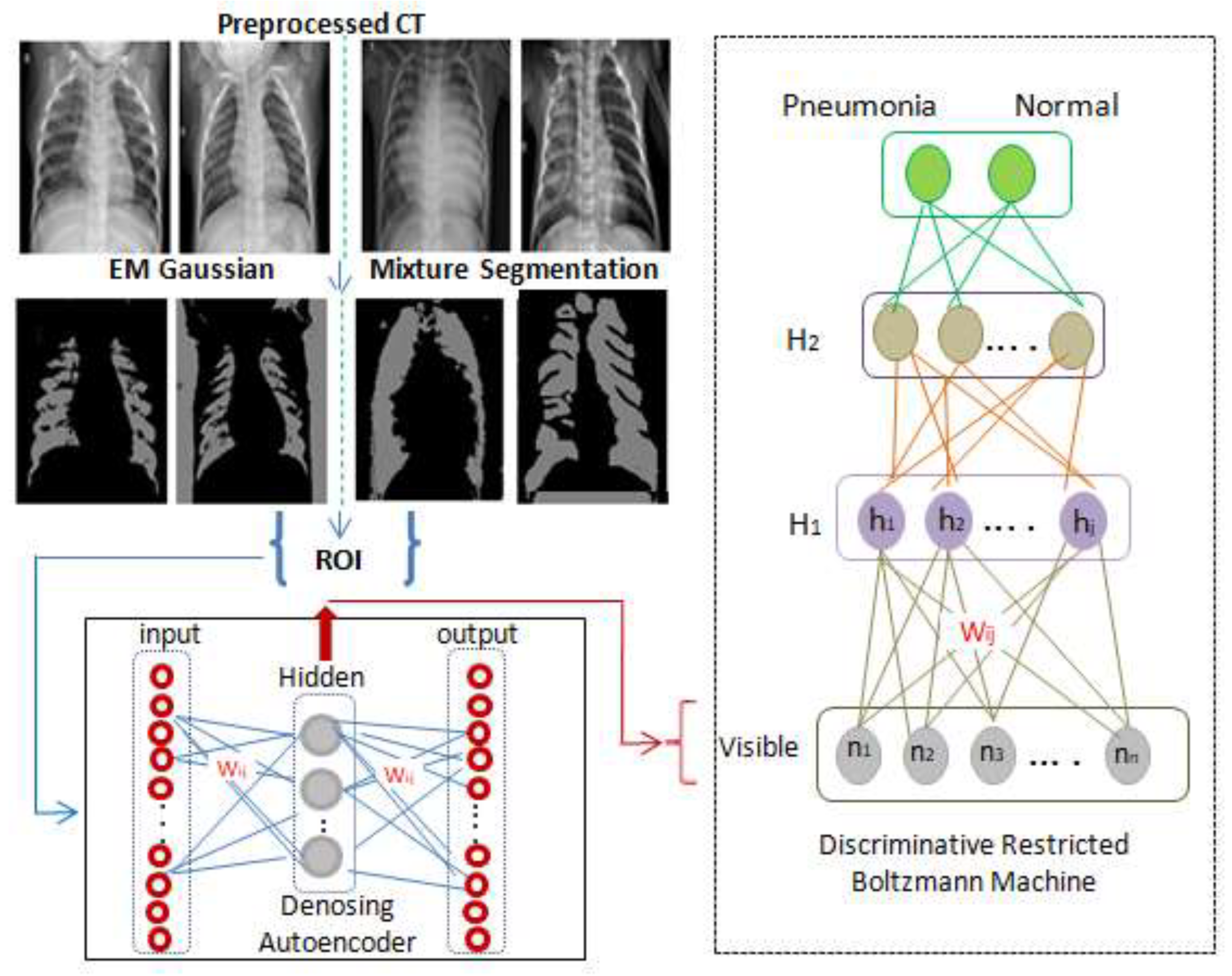
As seen in Figure 1, a classification layer that accepts weights from h₁ is added to the one hot vector of labels, and its back propagating error constructs an optimal regression layer to classify the scans to either class C₁ (pneumonia) or class C₂ (normal).

On the other hand, DRBM is a robust deep learning model [11] in which multiple RBMs are stacked in a graded way to robustly handle ambiguous input. The DBM is an undirected generative architecture that gathers features from lower and upper layers which enhances the representation scheme. A DRBM is constructed by sequencings multiple RBMs, where the input to the kth layer RBM is the learned feature representation from the RBM at the (k − 1)th layer.

4. Architecture and Development of the Proposed Model

This work proposes a hybrid model for the identification of pneumonia that combines DAE and DRBM to allow for a more powerful classification model. In order to overcome the dimensionality problem during the training phase of the AE convolution, the ROI is extracted from the input scans using the discussed EMGM model in Section 3.1.

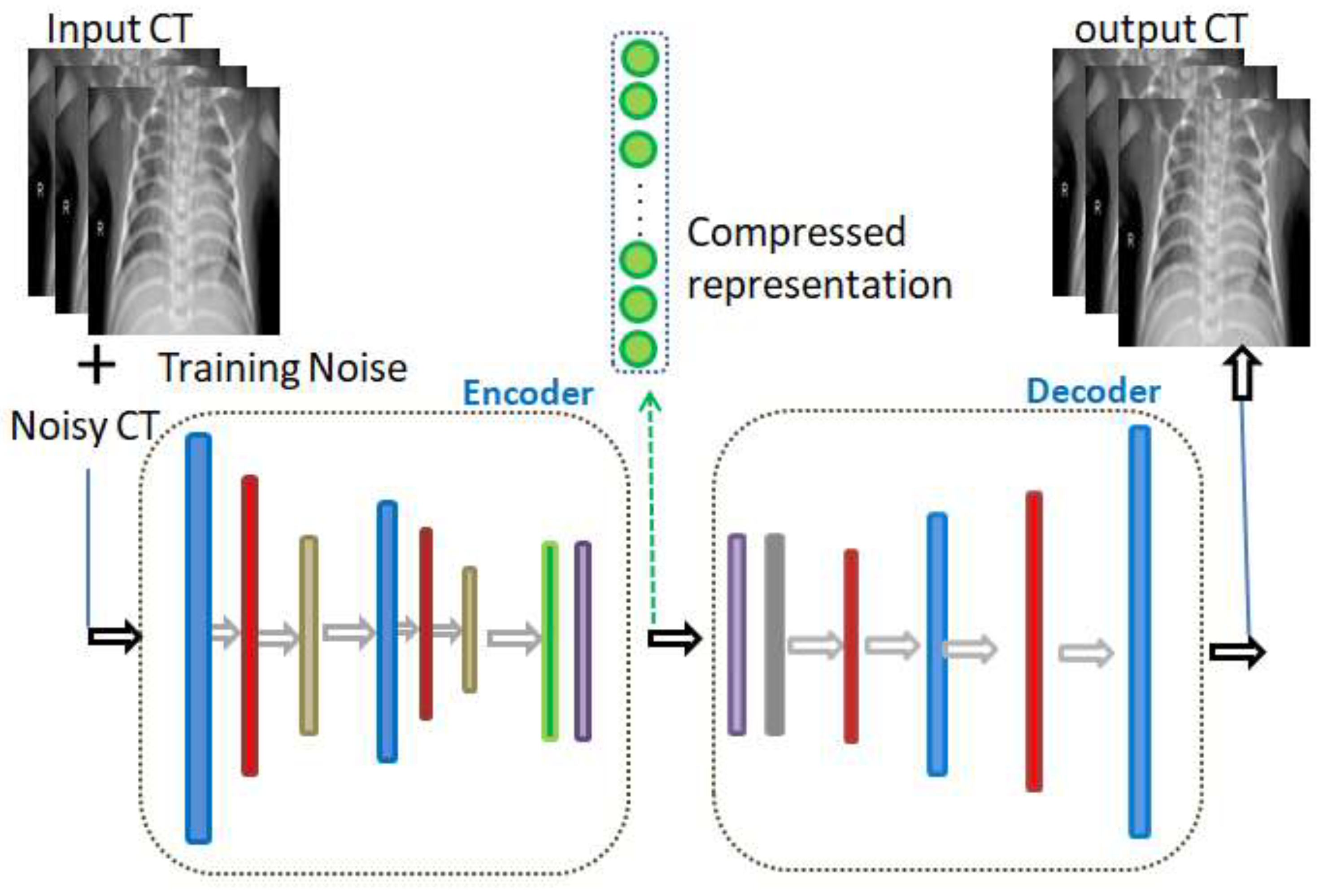
As illustrated in Figure 2, the colored layers of the DAE represent consequent convolutional, max pooling, batch normalization, and dense layers. The input noise exists in the AE training phase only, and not in the validation and testing phases. In fact, in view of the purpose of the model, the innermost flattening and dense layers may be omitted while composing its layers. The convolutional layer (colored in blue in Figure 1) is accountable for the extraction of the neighborhood features.

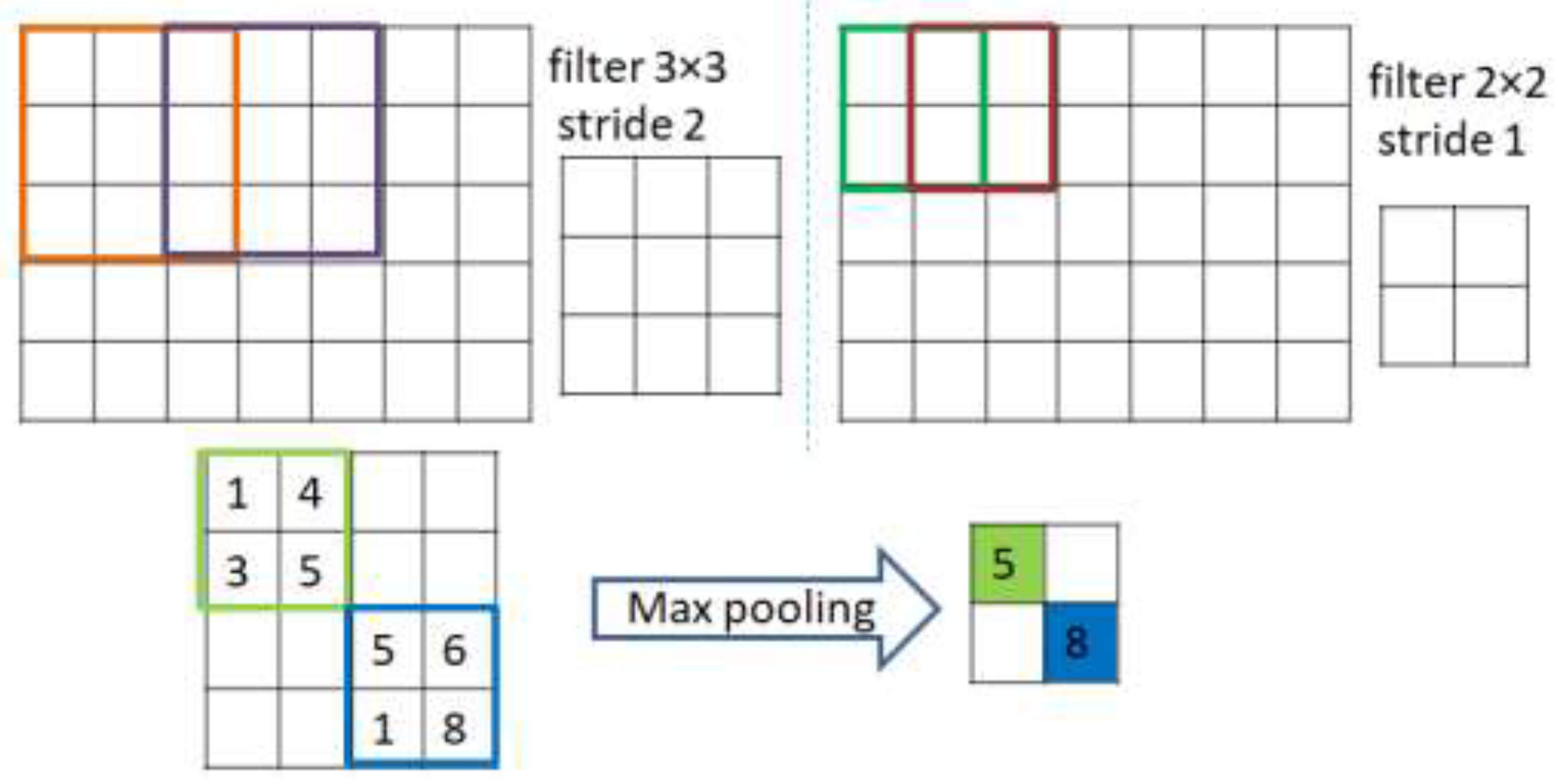
As shown in Figure 3, extraction is achieved through applying a number of kernels from the convolutions to construct a map of specific normalized features. In more precise terms, a kernel function is convolved with a pre-determined part of the image of identical kernel size to that of the output pixel. The kernel then slides by a certain distance, or stride length, this continues till it abstractly represents the entire image. The rectified linear unit (ReLU) acts as an activation function for the convolutional layers that maps the inputs to the output (omitting the last layer of the decoder that uses alternative, or sigmoid, activation). The batch normalization layer (colored with red in Figure 2) is responsible for the normalization step. This is a regular run on the output of the layer, by constraining a zero mean and a unit variance. Accordingly, it increases the balance of the network and speeds up the training. The dense layer is a fully connected group of neurons (each input neuron is connected to every output by a weight resulting from a nonlinear activation function). On the other hand, as shown in Figure 2, the decoding entails the identical layers of the encoder, although reversely ordered. Its first layer is the dense layer; however, when the encoder architecture does not contain a dense layer, then reshaping of the hidden vector occurs through the Reshape layer (colored in gray). Finally, the de-convolution and the up sampling of the image processes are performed by the de-convolution layer.

5. Case Study and Experimental Results

The experiments in this paper were implemented using Python, TensorFlow, keras, and Google Colab, which offer features of remote servers’ capabilities including a GPU (1× Tesla K80), (2496 CUDA), (12 GB) GDDR-5 V-RAM; a CPU (1× single core hyper threaded) Xeon Processors 2:3 Ghz, 45 MB Cache; and our personal laptop, which is an intel (R) core (TM) i7, 7200U processor 2:5 GHz and 16 GB of RAM.

5.1. Data Preprocessing and Augmentation

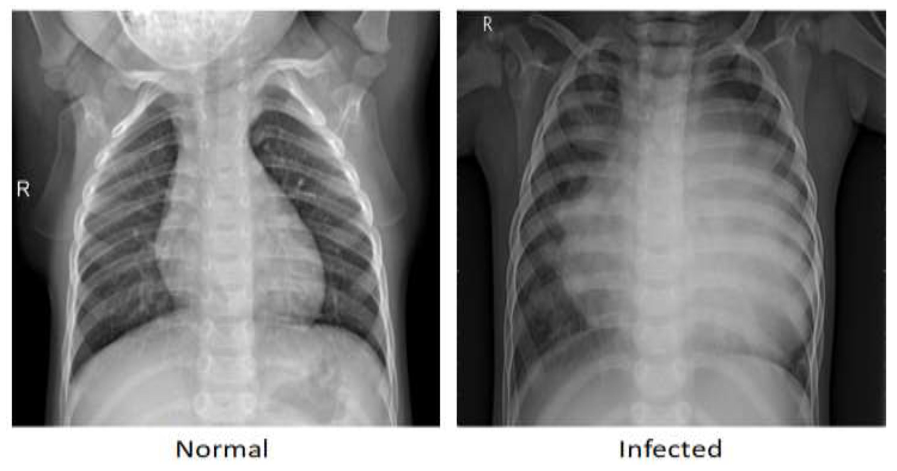
The proposed model is applied to a publicly available dataset of medical chest X-rays for pneumonia detection [34]. The digital computed radiography (CR) captured a total of 5856 images with 1583 normal cases and 4273 pneumonia cases. Figure 4 shows an example each of the CR scan for normal patients and for those diagnosed with pneumonia, in which the lungs in the normal scan are clear, while the lungs diagnosed with pneumonia look cloudy with a white area.

The data imbalance ration (IR) was measured using Equation (11). Since IR is 46% and the convolution developed model is complex, an augmentation process was mandatory to overcome the over-fitting issue.

$$\frac{\left|\mathrm{Support}\left({\mathrm{Normal}}_{\mathrm{class}}\right)-\mathrm{support}\left({\mathrm{Pneumonia}}_{\mathrm{class}}\right)\right|}{\mathrm{Support}\left({\mathrm{Normal}}_{\mathrm{class}}\right)+\mathrm{Support}\left({\mathrm{Pneumonia}}_{\mathrm{class}}\right)-\mathrm{support}\left({\mathrm{Normal}}_{\mathrm{class}}{{\displaystyle \cap }}^{\text{}}{\mathrm{Pneumonia}}_{\mathrm{class}}\right)}$$

(11)

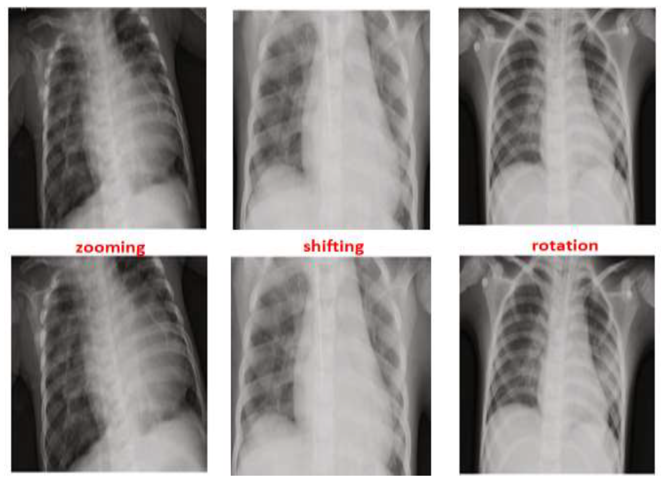
As seen in Figure 5, zooming, flipping, shifting and rotation operations were used in the augmentation process to balance the distribution of the scans between Normal and Pneumonia cases. After applying the augmentation process to the Normal class, the number of normal cases increased from 1583 cases to 7915 cases. By contrast, the augmentation process for the Pneumonia class was performed on 75% of the 4273 using only one operation from the augmentation operations that was selected randomly. This results in an increase of the Pneumonia cases reaching a new total of 7478. This led to the reduction in the IR of Normal and Pneumonia cases from 46% to 2.8%, which is considered a huge improvement.

Lastly, a preprocessing phase was considered so as to unify the resolution among the images in the dataset to all be (224 × 224). Thereafter, a normalization step was applied before injecting the images to our model.

Table 1. Data set distribution before and after augmentation and class balancing.

	Before Preprocessing			Generated Cases	Updated	After Preprocessing
Normal	Train	Test	Validate	6332	7915	Train	Test	Validate
	1341	234	8			5540	1978	397
	Total = 1583
Pneumonia	3875	390	8	3205	7478	5235	1870	373
	Total = 4273

shows the details of the updated cases in the dataset before and after preprocessing and the details of the distributed cases among the training (70%), testing (25%), and validation (5%) phases.

5.2. Feature Visualization and Model Results

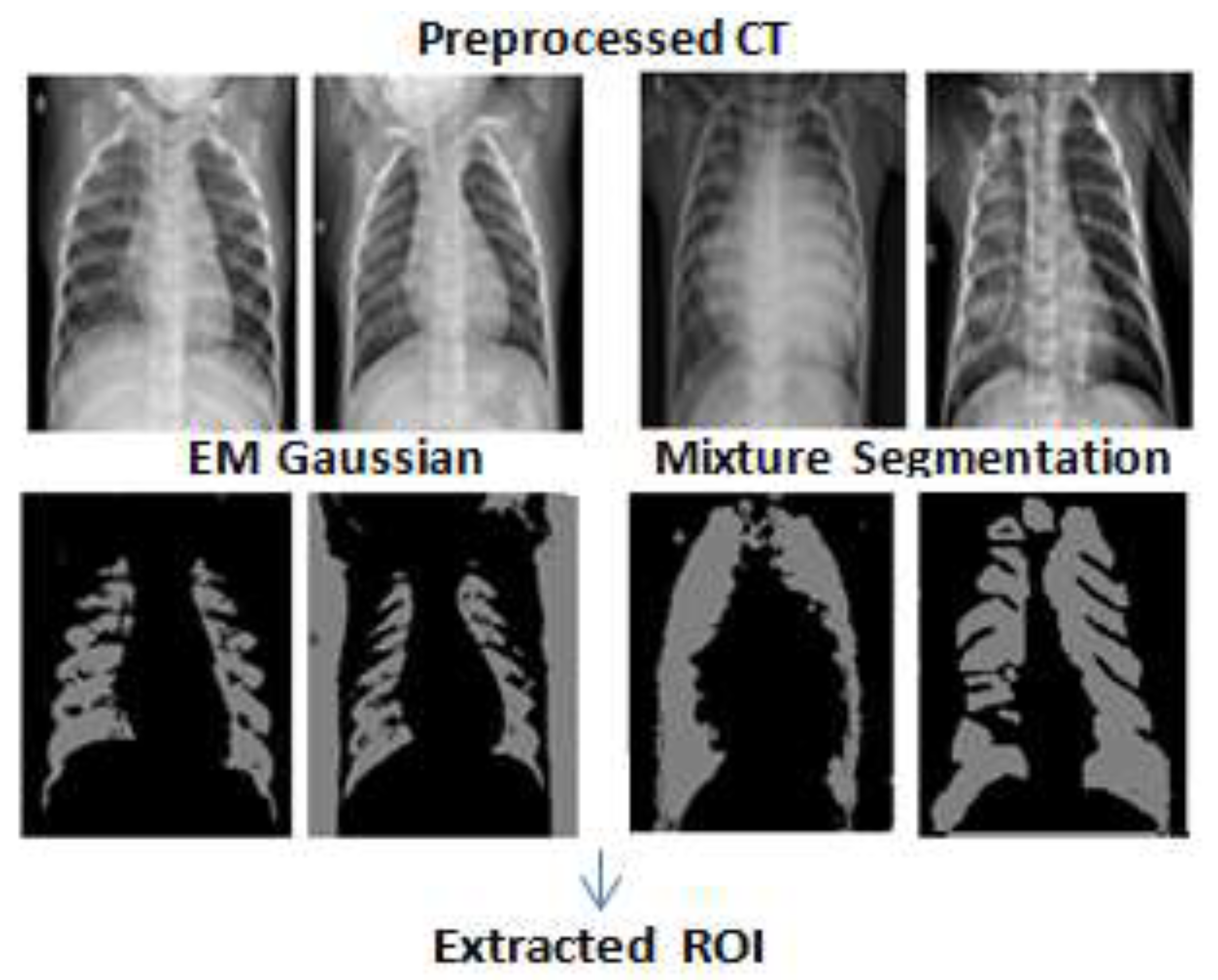
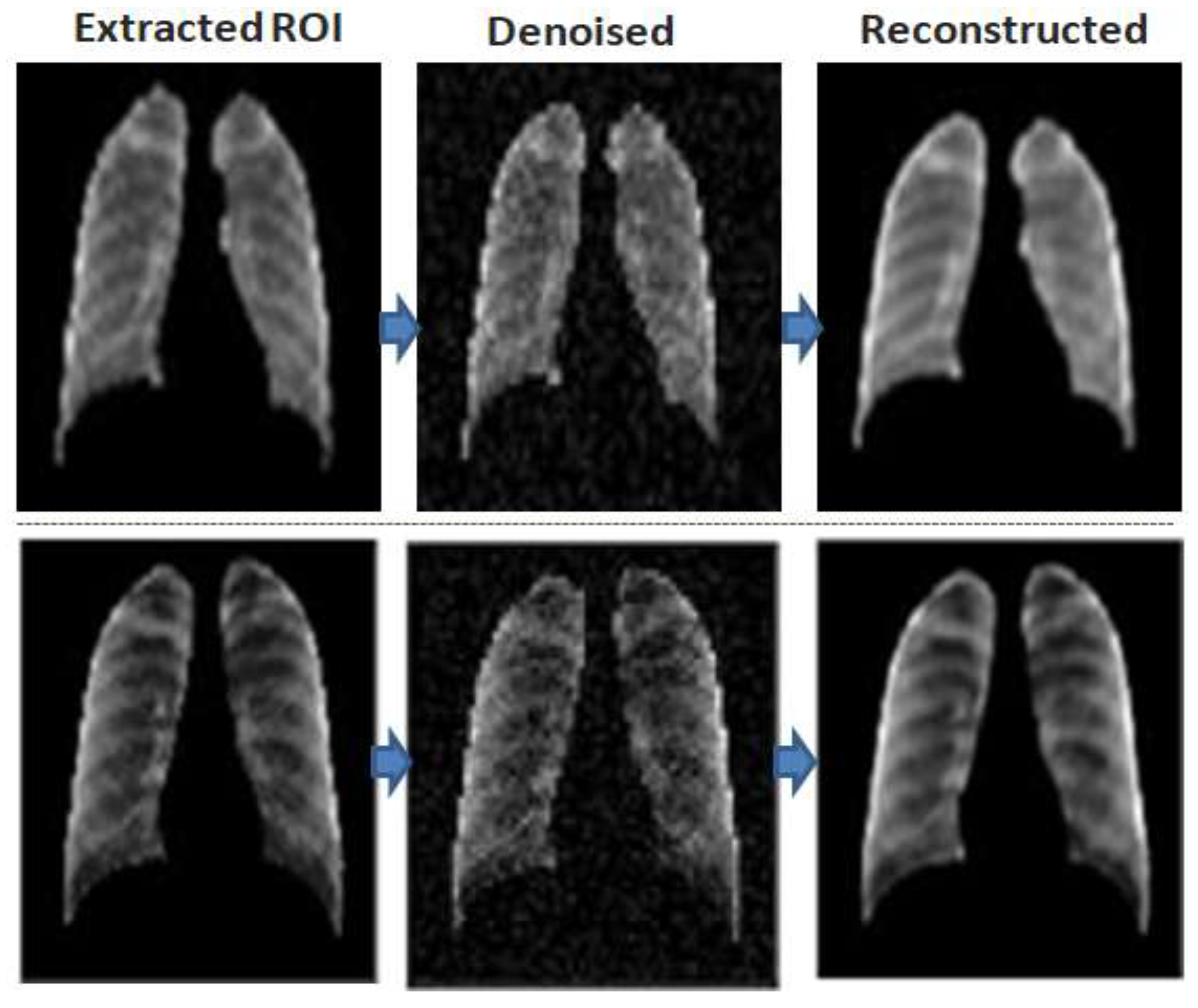
This section presents the entailed results from each phase of the proposed model as explained previously. The results from the segmentation phase using EMGMM to extract the ROI are shown in Figure 6, where the extracted ROI images are cropped and are fed to the training phase of the convolution denoising autoencoder (DAE) as shown in Figure 7.

As can be seen in Figure 7, the DAE minimized the error by reconstructing the input using stochastic transformation, which involves adding noise with a specific factor (0.01 in our experiment), and randomly sets some inputs to zero to obtain a set of corrupted images. Next, the DAE reconstructs the corrupted versions of images and extracts the features from them.

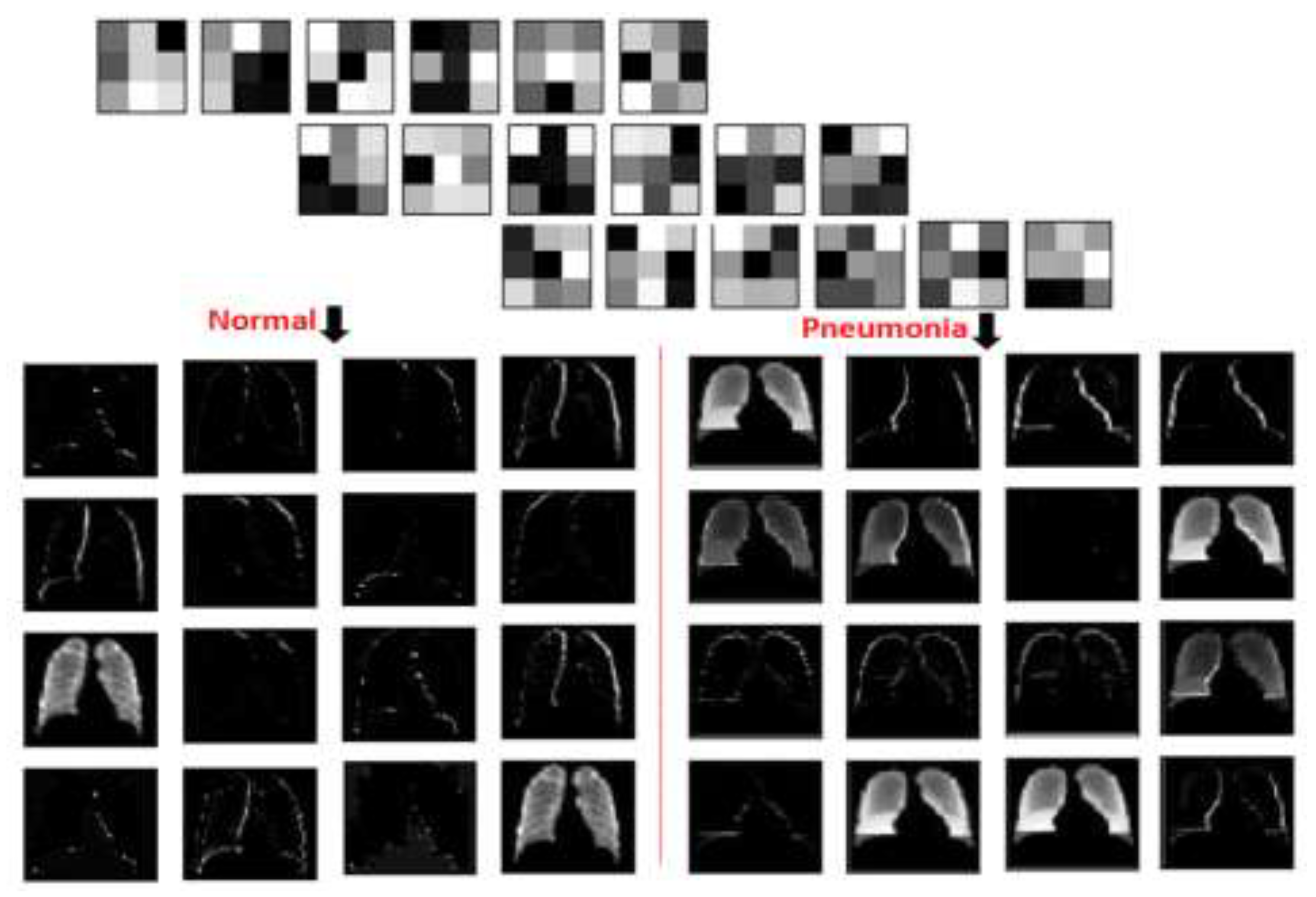
Adding the denoised factor of 0.01 guides the autoencoder to select the most valuable features and ignore the others, hence to reduce dimensionality and provide the unsupervised work to the RBM layer for the supervised classification task. This hybrid structure forces the model to learn in a more abstract way and to become more noise-resistant, which in turn helps with improving the performance, robustness, and generalization of results. A plotting for the used filter (3 × 3) and its features resulted in two-dimensional images, as seen in Figure 8, where a sample of such filters and features is visualized using one normal case and one pneumonia case, respectively.

5.3. Adding DRBM Classifier

After the DAE training, the weights were transferred to the deep restricted Boltzmann machine (DRBM) that contains two hidden layers. The input values for the DRBM depend on the dimensions of weights from the denoising encoder. See

Table 2. Denoising autoencoder layer parameters: kernel size, stride and output dimensions.

Layers	Filter Size	Stride	Output Dimension
Conv2D	3 × 3	2	224 × 224 × 128
Batch Normalization	-	-	224 × 224 × 128
Conv2D	3 × 3	1	224 × 224 × 64
MaxPooling	2 × 2	2	112 × 112 × 64
Con2D	3 × 3	1	112 × 112 × 32
Batch Normalization	-	-	112 × 112 × 32
MaxPooling	2 × 2	2	56 × 56 × 32

for details of kernel layers, strides and dimensions.

Before the training started, some hyperparameters were set (e.g., fine-tuning learning rates = 0.015, stop training = 100 epochs, and fine tuning = of 500 epochs). The number of inputs to the model was 3136. The number of visible units was set to 224 × 224 nodes. These were connected to 750 nodes in the first hidden layer. Once the DRBM learns the structure of the input data, the data is transferred one layer down the net, hence it is mapped to 100 in the second hidden layer. This approach of constructing sequential sets of activations by clustering the features, and then clustering the clusters of features, is the main function of the feature map; through this approach, the model learns more complicated but summarized representations of data.

Additionally, a normal distribution with mean = 0 and variance = 1 is used to randomly set the DRBM initial parameters. Later, a fully connected and a dense layer are added to classify Normal and Pneumonia cases. With reference to the characteristics of the autoencoder: it is not able to deal with categorical attributes; accordingly, data labels were converted into one-hot encoding. In this implementation, two classes are considered: Normal and Pneumonia. Two Boolean columns for the two mentioned classes were mapped, and we then set a value of 1 to indicate the class label for every sample in only one column. The DRBM records satisfactory learning and discriminative representation from epoch 15. Hence, the autoencoder enhanced learning of features through the transfer of their weights. Afterward, on reaching epoch 50, the enhancement in the learning rate slowed down with respect to the epoch’s number. The proposed hybrid model resulted in a recognition rate of 98.63%.

5.4. Evaluation and Analysis of Results

To evaluate the model, cross validation was used as this is considered as the main measure for the classifier performance and generalization. For the cross validation, the obtained ROIs were organized in 10 folds keeping a balanced class distribution of Normal and Pneumonia cases. The accuracy values for the cross-validation of all the 10-fold experiments were recorded. In each run, one fold was used for testing and the other nine folds were used for training and tuning. We then calculated the mean accuracy, accuracy, sensitivity, and specificity and compared these with the performance of other models that were applied to the same dataset, as seen in

Table 3. Comparison analysis of different methods for feature selection and classifiers.

Author	Learning Technique	Features Method	Accuracy
[35]	Deep Siamese based neural network	CNN	89.6%
[36]	CNN	CNN	96.65%
[37]	CNN	Multiple features	98.46%
	Rain forest		97.6%
	KNN		92.5%
	Adaboost		95.6%
[38]	CNN + transfer learning (AlexNet)	CNN	94.5%
	ResNet18		96.4%
	DenseNet201		98%
	SqueezeNet		96.1%
Proposed model	Hybrid of denoising autoencoder + DRBM	Denoising autoencoder	98.63%

. It can be noted that our proposed model achieved the highest accuracy (98.63%) between them.

The Confusion Matrix is another important measure for the evaluation of the hybrid model. Accordingly, True Positive (TP: the correct classification of pneumonia existence), True Negative (T_n: correct classification of normal), False Positive (F_P: the misclassified existence of pneumonia), and False Negative (F_n: the misclassified of normal cases) were computed for the model. Next, sensitivity (S_e), specificity (S_p), positive predictive value (PP_V) and classification accuracy (ACC) were calculated to provide deeper insight into the performance of the classifier [see Equations (12)–(15)].

$${\mathrm{s}}_{\mathrm{e}}=\frac{{\mathrm{T}}_{\mathrm{p}}}{{\mathrm{T}}_{\mathrm{p}}+{\mathrm{T}}_{\mathrm{n}}}\times 100$$

(12)

$${\mathrm{s}}_{\mathrm{p}}=\frac{{\mathrm{T}}_{\mathrm{n}}}{{\mathrm{T}}_{\mathrm{n}}+{\mathrm{F}}_{\mathrm{p}}}\times 100$$

(13)

$${\mathrm{PP}}_{\mathrm{v}}=\frac{{\mathrm{T}}_{\mathrm{p}}}{{\mathrm{T}}_{\mathrm{p}}+{\mathrm{F}}_{\mathrm{p}}}\times 100$$

(14)

$$\mathrm{ACC}=\frac{{\mathrm{T}}_{\mathrm{p}}+{\mathrm{T}}_{\mathrm{n}}}{{\mathrm{T}}_{\mathrm{p}}+{\mathrm{T}}_{\mathrm{n}}+{\mathrm{F}}_{\mathrm{p}}+{\mathrm{F}}_{\mathrm{n}}}\times 100$$

(15)

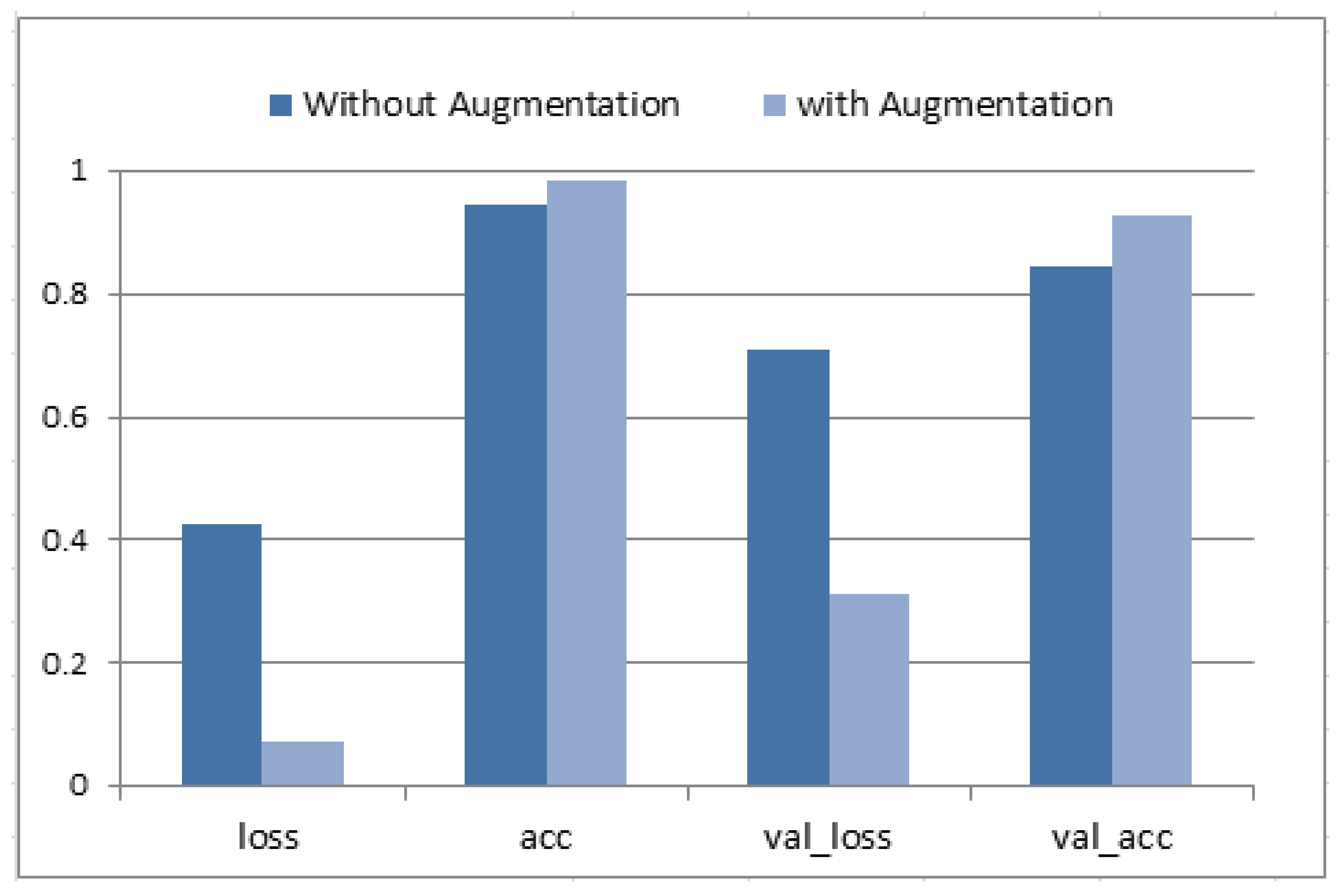
Figure 9 presents the hybrid model training and validation accuracy. The optimal performance was reported at epoch #100 (each of 20 steps). Then, the classification accuracy, loss, validation accuracy and validation loss were written down for two cases (with augmentation and without augmentation). An average accuracy of 94.71%, sensitivity of 93.3%, and specificity of 92.4% were obtained without augmentation. Data augmentation enhanced the average accuracy as it allowed it to reach the value of 98.63%, sensitivity of 96.5%, and specificity of 94.8%. Moreover, both values for val_loss and val_accuracy were improved.

6. Conclusions and Future Work

In this paper, we introduced a new hybrid deep convolution model for the diagnosis of pneumonia infection from CT scans of patients’ lungs. The model integrates both the DAE and the DRBM in the classification and prediction processes, and uses EMGMM to extract the ROI segments. The dataset that was considered in this work consists of 5856 images with 1583 normal cases and 4273 pneumonia cases, and an IR of 0.46. An augmentation process including rotation, flipping, shifting, and zooming was implemented to enhance the balance of the data, which yielded 4273 images with a better IR of 0.028. A 10-fold cross validation was used for testing and validation purposes. Accuracy, loss, validation accuracy and validation loss were measured with and without augmentation. Results showed an average accuracy of 94.71%, sensitivity of 93.3%, and specificity of 92.4% without the augmentation process, and an average accuracy of 98.63%, sensitivity of 96.5%, and specificity of 94.8% after augmentation. As seen previously in Table 3, our proposed model achieved the highest accuracy value over other models that were applied to the same dataset—among which the previously highest reported accuracy in the literature was 98.46% using regular CNN with hyperparameters. Possible applications of this model are its integration into a computer-based system to detect and/or predict the type of infection with high accuracy—COVID-19 versus SARS-CoV-2 versus others. This model can also be used in portable chest X-ray devices in airports as an in-time detector for COVID-19 instead of the PCR test, or used in athletics before competitions or training especially divers, footballers, and other sports that require a healthy respiratory system to avoid serious illness or catastrophic death.

References

- Lakhani, P.; Sundaram, B. Deep learning at chest radiography: Automated classification of pulmonary tuberculosis by using convolutional neural networks. Radiology 2017, 284, 574–582. [Google Scholar] [CrossRef]
- Krishnamurthy, S.; Srinivasan, K.; Qaisar, S.M.; Vincent, P.D.R.; Chang, C.Y. Evaluating Deep Neural Network Architectures with Transfer Learning for Pneumonitis Diagnosis. Comput. Math Methods Med. 2021, 8036304. [Google Scholar] [CrossRef]
- Siddiqi, R. Automated pneumonia diagnosis using a customized sequential convolutional neural network. In Proceedings of the 2019 3rd International Conference on Deep Learning Technologies, Xiamen, China, 5–7 July 2019; pp. 64–70. [Google Scholar] [CrossRef]
- Račić, L.; Popović, T.; Čakić, S.; Šandi, S. Pneumonia Detection Using Deep Learning Based on Convolutional Neural Network. In Proceedings of the 25th International Conference on Information Technology (IT), Zabljak, Montenegro, 16–21 February 2021; pp. 1–4. [Google Scholar] [CrossRef]
- Stephan, E.; Schlagenhaut, F.; Huys, Q.; Raman, S.; Aponte, E.; Brodersen, K.; Rigoux, L.; Moran, R.; Daunizeau, J.; Dolan, R.; et al. Computational neuroimaging strategies for single patient predictions. Neuroimage 2017, 145, 180–199. [Google Scholar] [CrossRef] [Green Version]
- Schmidhuber, J. Deep learning in neural networks: An overview. Neural Netw. 2015, 61, 85–117. [Google Scholar] [CrossRef] [Green Version]
- Krizhevsky, A.; Sutskever, I.; Hinton, G. ImageNet classification with deep convolutional neural networks. In Proceedings of the Advances in Neural Information Processing Systems; MIT Press: Cambridge, MA, USA, 2012; pp. 1106–1114. [Google Scholar]
- Cai, Y.; Landis, M.; Laidley, D.; Kornecki, A.; Lum, A.; Li, S. Multi-modal vertebrae recognition using transformed deep convolution network. Comput. Med. Imaging Graph. 2016, 51, 11–19. [Google Scholar] [CrossRef]
- Xu, J.; Xiang, L.; Liu, Q.; Gilmore, H.; Wu, J.; Tang, J. Stacked sparse autoencoder (SSAE) for nuclei detection on breast cancer histopathology images. IEEE Trans. Med. Imaging 2016, 35, 119–130. [Google Scholar] [CrossRef] [Green Version]
- Tsanev, G.S. Deep Multiconnected Boltzmann Machine for Classification. Am. J. Eng. Res. 2017, 6, 186–194. [Google Scholar]
- Salakhutdinov, R.; Hinton, G. An efficient learning procedure for deep Boltzmann machines. Neural Comput. 2012, 24, 1967–2006. [Google Scholar] [CrossRef] [Green Version]
- Larochelle, H.; Bengio, Y. Classification using discriminative restricted boltzmann machines. In Proceedings of the ACM International Conference on Machine Learning, Helsinki, Finland, 5–9 July 2008; pp. 536–543. [Google Scholar]
- Salakhutdinov, R.; Hinton, G. Deep Boltzmann machines. In Artificial Intelligence and Statistics; PMLR: Fort Lauderdale, FL, USA, 2009; pp. 448–455. [Google Scholar]
- Sankaran, A.; Goswami, G.; Vatsa, M.; Singh, R.; Majumdar, A. Class sparsity signature based restricted boltzmann machine. Pattern Recognit. 2017, 61, 674–685. [Google Scholar] [CrossRef]
- Li, D.; Fu, Z.; Xu, J. Stacked-autoencoder-based model for COVID-19 diagnosis on CT images. Int. J. Res. Intell. Syst. Real Life Complex Probl. 2021, 51, 2805–2817. [Google Scholar] [CrossRef]
- Vincent, P.; Larochelle, H.; Bengio, Y.; Manzagol, P. Extracting and composing robust features with denoising autoencoders. In Proceedings of the 25th International Conference on Machine Learning, Helsinki, Finland, 5–9 July 2008; pp. 1096–1103. [Google Scholar]
- Gomes, J.; Masood, A.; da Silva, L.H.S.; da Cruz Ferreira, J.R.B.; Freire Junior, A.A.; dos Santos Rocha, A.L. COVID-19 diagnosis by combining RTPCR and pseudo-convolutional machines to characterize virus sequences. Sci. Rep. 2021, 11, 11545. [Google Scholar] [CrossRef] [PubMed]
- Iwendi, C.; Mahboob, K.; Khalid, Z.; Javed, A.; Rizwan, M.; Ghosh, U. Classification of COVID-19 individuals using adaptive neuro-fuzzy inference system. Multimed. Syst. 2022, 28, 1223–1237. [Google Scholar] [CrossRef] [PubMed]
- Yee, S.; Raymond, W. Pneumonia Diagnosis Using Chest X-ray Images and Machine Learning. In Proceedings of the 10th International Conference on Biomedical Engineering and Technology (ICBET 20), Tokyo, Japan, 15–18 September 2020; pp. 101–105. [Google Scholar]
- Hashmi, M.F.; Katiyar, S.; Keskar, A.G.; Bokde, N.D.; Geem, Z.W. Efficient Pneumonia Detection in Chest Xray Images Using Deep Transfer Learning. Diagnostics 2020, 10, 417. [Google Scholar] [CrossRef]
- Chouhan, V.; Singh, S.K.; Khamparia, A.; Gupta, D.; Tiwari, P.; Moreira, C.; Damaševičius, R.; Alburquerque, V.H. A Novel Transfer Learning Based Approach for Pneumonia Detection in Chest X-ray Images. Appl. Sci. 2020, 10, 559. [Google Scholar] [CrossRef] [Green Version]
- Mahmud, T.; Rahman, M.; Fattah, S. CovXNet: A multi-dilation convolutional neural network for automatic COVID-19 and other pneumonia detection from chest X-ray images with transferable multi-receptive feature optimization. Comput. Biol. Med. 2020, 1, 122. [Google Scholar] [CrossRef]
- Abiyev, R.H.; Ma’aitah, M.K.S. Deep convolutional neural networks for chest diseases detection. J. Healthc. Eng. 2018, 2018, 4168538. [Google Scholar] [CrossRef] [Green Version]
- Stephen, O.; Sain, M.; Maduh, U.J.; Jeong, D. An efficient deep learning approach to pneumonia classification in healthcare. J. Healthc. Eng. 2019, 2019, 1–7. [Google Scholar] [CrossRef] [Green Version]
- Kundu, R.; Das, R.; Geem, Z.W.; Han, G.-T.; Sarkar, R. Pneumonia detection in chest X-ray images using an ensemble of deep learning models. PLoS ONE 2021, 16, e0256630. [Google Scholar] [CrossRef]
- Yao, J.C.; Wang, T.; Hou, G.H.; Ou, D.; Li, W.; Zhu, Q.D.; Chen, W.C.; Yang, C.; Wang, L.J.; Wang, L.P.; et al. AI detection of mild COVID-19 pneumonia from chest CT scans. Eur. Radiol. 2021, 31, 7192–7201. [Google Scholar] [CrossRef]
- Wang, C.; Elazab, A.; Jia, F.; Wu, J.; Hu, Q. Automated chest screening based on a hybrid model of transfer learning and convolutional sparse denoising autoencoder. Biomed. Eng. 2018, 17, 63. [Google Scholar] [CrossRef]
- Dhahri, H.; Rabhi, B.; Chelbi, S.; Almutiry, O.; Mahmood, A.; Alimi, A.M. Automatic Detection of COVID-19 Using a Stacked Denoising Convolutional Autoencoder. CMC-Comput. Mater. Contin. 2021, 69, 3259–3274. [Google Scholar] [CrossRef]
- Farnoosh, R.; Zarpak, B. Image segmentation using Gaussian mixture model. IUST Int. J. Eng. Sci. 2008, 19, 29–32. [Google Scholar]
- Hui, B.; Guanyu, Y.; Huazhong, S.; Dillenseger, J. Accurate Image Segmentation Using Gaussian Mixture Model with Saliency Map. In Pattern Analysis and Applications; Springer: Berlin/Heidelberg, Germany, 2018; Volume 21, pp. 869–878. [Google Scholar]
- Goodfellow, I.; Bengio, Y.; Courville, A. Deep Learning; MIT Press: Cambridge, MA, USA, 2016. [Google Scholar]
- Masci, J.; Meier, U.; Cireşan, D.; Schmidhuber, J. Stacked convolutional autoencoders for hierarchical feature extraction. In Artificial Neural Networks and Machine Learning. ICANN 2011; Lecture Notes in Computer Science; Springer: Berlin/Heidelberg, Germany, 2011; Volume 6791, pp. 52–59. [Google Scholar]
- Vincent, P.; Larochelle, H.; Lajoie, I.; Bengio, Y.; Manzagol, P.A. Stacked denoising autoencoders: Learning useful representations in a deep network with a local denoising criterion. J. Mach. Learn. Res. 2010, 11, 3371–3408. [Google Scholar]
- Kaggle, P.M. Kaggle’s Chest X-ray Images (Pneumonia) Dataset. 2020. Available online: https://www.kaggle.com/paultimothymooney/chest-xray-pneumonia (accessed on 30 January 2022).
- Acharya, A.; Satapathy, R. A Deep Learning Based Approach towards the Automatic Diagnosis of Pneumonia from Chest Radio-Graphs. Biomed. Pharmacol. J. 2020, 13, 449–455. [Google Scholar] [CrossRef]
- Tobias, R.; De Jesus, L.C.M.; Mital, M.; Lauguico, S.; Guillermo, M.; Sybingco, E.; Bandala, A.; Dadios, E. CNN-based Deep Learning Model for Chest X-ray Health Classification Using TensorFlow. In Proceedings of the International Conference on Computing and Communication Technologies, Ho Chi Minh City, Vietnam, 14–15 October 2020. [Google Scholar]
- Emhamed, R.; Mamlook, A.; Chen, S. Investigation of the performance of Machine Learning Classifiers for Pneumonia Detection in Chest X-ray Images. In Proceedings of the IEEE International Conference on Electro Information Technology (EIT’ 20), Chicago, IL, USA, 31 July–1 August 2020; pp. 98–104. [Google Scholar]
- Rahman, T.; Chowdhury, M.; Islam, K.; Islam, K.; Mahbub, Z.; Kadir, M.; Kashem, S. Transfer Learning with Deep Convolutional Neural Network (CNN) for Pneumonia Detection Using Chest X-ray. Appl. Sci. 2020, 10, 3233. [Google Scholar] [CrossRef]