High-Frequency Forecasting of Stock Volatility Based on Model Fusion and a Feature Reconstruction Neural Network

Abstract

Stock volatility is an important measure of financial risk. Due to the complexity and variability of financial markets, time series forecasting in the financial field is extremely challenging. This paper proposes a “model fusion learning algorithm” and a “feature reconstruction neural network” to forecast the future 10 min volatility of 112 stocks from different industries over the past three years. The results show that the model in this paper has higher fitting accuracy and generalization ability than the traditional model (CART, MLR, LightGBM, etc.). This study found that the “model fusion learning algorithm” can be well applied to financial data modeling; the “feature reconstruction neural network” can well-model data sets with fewer features.

1. Introduction

In recent years, time series models have been explored to solve various engineering application problems. With the rise of the big data industry, the combination of big data and the financial field has formed big data finance [1,2,3]. Time series forecasting of financial indicators has become a widely studied topic in recent years. However, the highly complex, highly time-varying, and highly nonlinear nature of data in the financial sector makes the forecasting of relevant indicators more challenging [4]. In financial markets, investors are more concerned with forecasting future market trends than accurate price forecasts. Volatility reflects the magnitude of price fluctuations, and volatility is a measure of asset price variability using high-frequency data information [5]. Volatility has extremely important decision-making value in risk management, option pricing, asset allocation, etc. Accurate forecasting of volatility can reduce uncertainty in investment decisions and improve investment efficiency for financial firms and investors [6]. Volatility has become one of the most important quantitative indicators in the current financial industry [7]. Therefore, the prediction model of volatility is of great academic and practical research importance.

1.1. Literature Review

In 1959, Osborme proposed the random walk theory which infers that stock prices are unpredictable [8]. In 1970, Fama’s efficient market hypothesis also inferred that stock prices could not be efficiently predicted [9]. However, in 1999, the nonrandom walk theory proposed by Lo and Mackinlay argued that stock prices could be predicted by economic modeling [10]. In 1971, Barclays Investment Management in the United States issued the world’s first fund using quantitative investment strategies [11]. The explosive growth and huge development prospects of the current global quantitative trading market have made stock-related time series forecasting a hot research topic [12].

In past studies by numerous scholars and experts on time series models and the prediction of stock volatility, different researchers have proposed different modeling schemes. Depending on the research area, the models can be broadly classified into two types: statistical models and machine learning models.

In the field of economics, volatility is often predicted using statistical models, which are knowledge paradigms that focus on theoretical perfectionism (data–knowledge–problem). The autoregressive conditional heteroskedasticity (ARCH) model was first proposed by Engle in 1982 and used for volatility forecasting [13]. The model was widely used in the field of time series forecasting because it was able to obtain good forecasting results for future information by using the variance function. By analyzing the actual situation, we can find that most time series forecasting research objects (such as stock volatility) will be affected by macroeconomics, national policies, company management, and other factors, and there will be strong randomness and sudden changes in future information. Based on this, in 1986, Bollerslev extended the variance function and further improved the ARCH model into a generalized autoregressive conditional heteroskedasticity (GARCH) model [14]. In 2005, Awartani and Corradi proposed that symmetric and asymmetric GARCH is applicable to symmetric and asymmetric stock volatility forecasting [15]. In 2021, Feng He and Libo Yin experimentally argued that linear regression models can also be effective in predicting stock volatility [16].

With the development of the computing performance of data centers and the improvement of financial markets, the data generated from real-time transactions and quantitative statistics have become more and more accurate, and financial big data with a precision of seconds is now commonly formed. High-frequency volatility has different characteristics than low-frequency volatility, with a negative correlation of time series, periodic U-shape, calendar effect, and long memory while the classical models based on low-frequency data (ARCH, SV, and GARCH) are difficult to use for the analysis of high-frequency data.

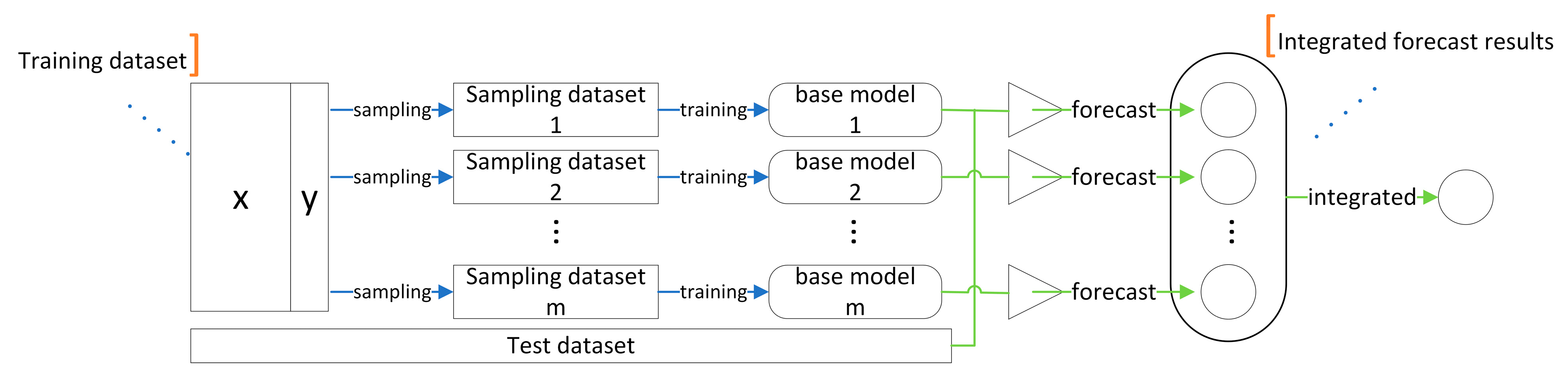
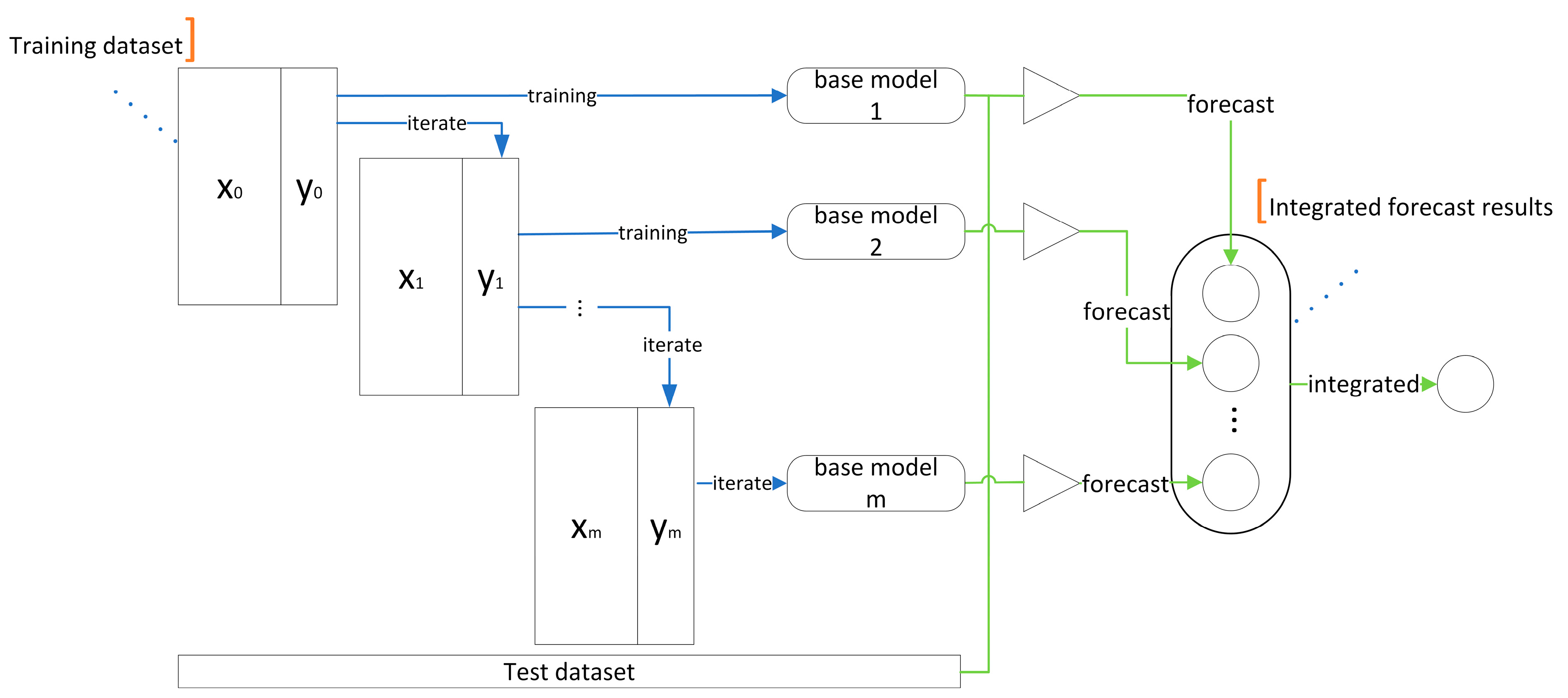
With the rise of artificial intelligence, machine learning has begun to be applied to solve various engineering challenges. While econometric models focus on being logic-driven, AI models focus more on being data-driven (data-problem), which is a kind of historical empiricism. In 2017, Li et al. accurately predicted the long- and short-term prices of copper using a regression tree model [17]. With the development of machine learning, many scholars have shifted their attention from single models to ensemble learning models, which have proven to be powerful performance metalearning algorithms, such as boosting and bagging. In 2016, Khaidem successfully forecasted stock returns by building a random forest model using the bagging algorithm on a decision tree model. In 2019, Basak, S. et al. implemented gradient-boosting decision trees (GBDT) using the distributed computing framework XGBoost and demonstrated that the GBDT (decision tree and boosting) algorithm outperformed random forests in the forecasting of stock volatility [18]. In 2022, Raubitzek and Neubauer et al. validated the powerful performance and advantages of GBDT in time series modeling (e.g., stock forecasting) [19].

Artificial neural networks (ANN) and deep learning frameworks have been hot research topics in artificial intelligence in recent years. Deep learning is a feature learning approach that converts raw data into a higher-level, more abstract representation process through a set of simple transformation methods, that is, using enough simple transformation functions and their various combinations to learn a complex objective function. It was found that any finite continuous function can be approximated by artificial neural networks, so artificial neural nets have fewer restrictions on model training and work well for regression fitting of both linear and nonlinear relationships. In 1988, White et al. 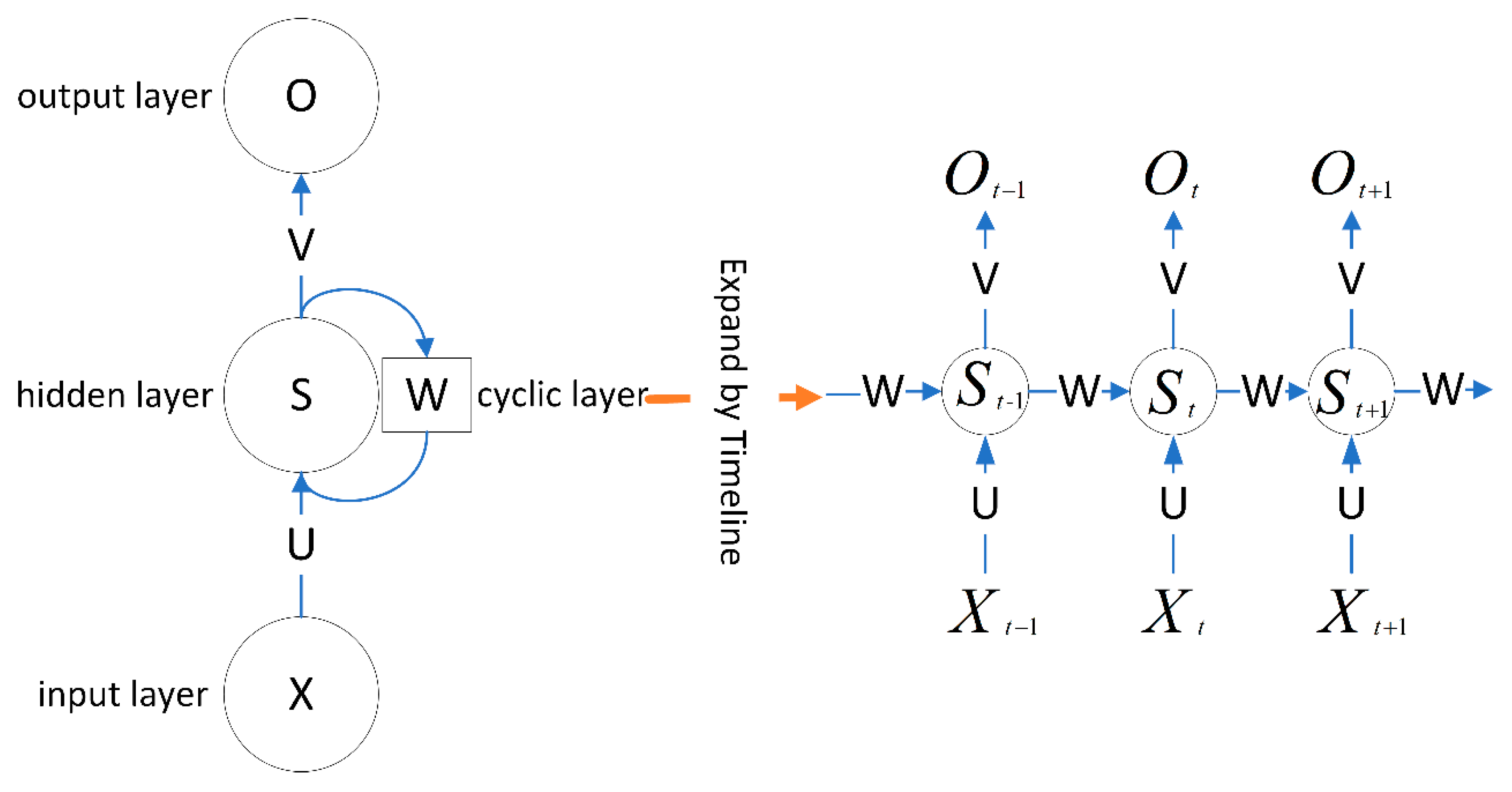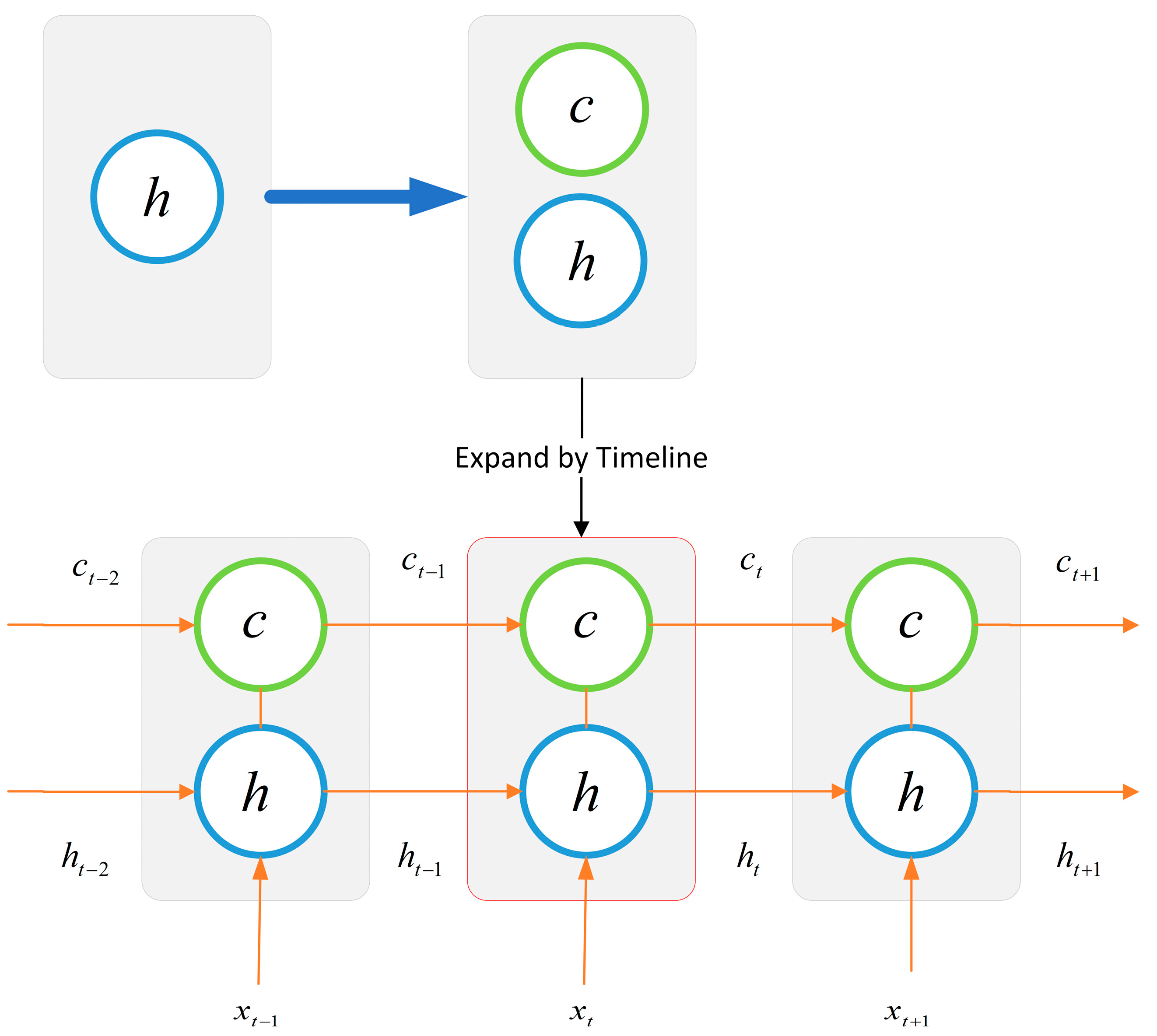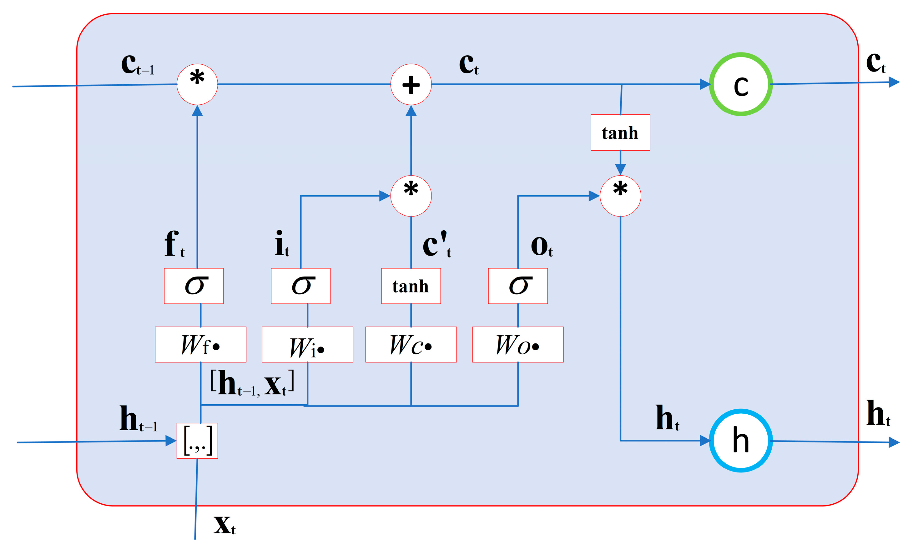used artificial neural networks to successfully predict the daily volatility of IBM stock [20]. However, the strong randomness and dynamic nonlinearity of financial big data make the fit of ordinary neural networks poor, and in 1997, Hochreiter et al. proposed the long short-term memory neural network (LSTM) [21]. The LSTM can store temporal information and has proven to be a very successful deep learning framework in various engineering applications of time series modeling. The LSTM is a kind of recurrent neural network (RNN). Unlike feedforward neural networks, recurrent neural networks have the mode of learning time through feedback connections, so RNNs have unique advantages in modeling and analyzing data of time series. Based on the advantages of LSTM, many scholars have successfully applied it to the forecasting research of financial indicators. In 2012, Maknickiene and Maknickas improved the prediction performance of feedforward neural networks using LSTM models and demonstrated that RNN models outperformed CNN models for the prediction of financial data information [22]. In 2015, Chen predicted the returns of the Chinese stock market by LSTM modeling [23]. In 2017, Nelson et al. used an LSTM model to predict the volatility of the stock market [24].

1.2. The Study of this Paper

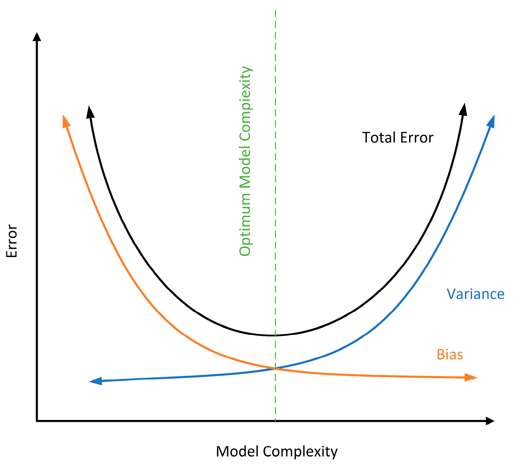
In the current research on time series models, although the relevant algorithms proposed by the above scholars have achieved good results, there are still some problems to be solved: (1) Initially, scholars used single machine learning for training, and the prediction error was relatively high. In recent years, ensemble learning models have been used to iteratively optimize the models, such as bagging to reduce variance and boosting to reduce bias, but there is no way to reduce both bias and variance. (2) If a neural network is directly used for training, the model has poor interpretability and high uncertainty, the increase of input parameters will cause the model complexity to be too high, and the time and computational resources consumed for model training are not optimistic. (3) Before the era of artificial intelligence, the contradiction of intelligent algorithms was between the lack of algorithms and the growing demand for algorithms from users. With the development of artificial intelligence and big data, the contradiction of intelligent algorithms becomes a contradiction between the limited versatility of algorithms and the diversity of engineering problems. Although this is an era of algorithm enrichment, there is no perfect algorithm and no universal model. In 1997, Wolpert and Macready proposed the “no free lunch” theorem that no single model can provide the most accurate predictions for all time series data and that specific modeling approaches must be found for specific problems because universal solutions are unlikely to emerge [25,26].

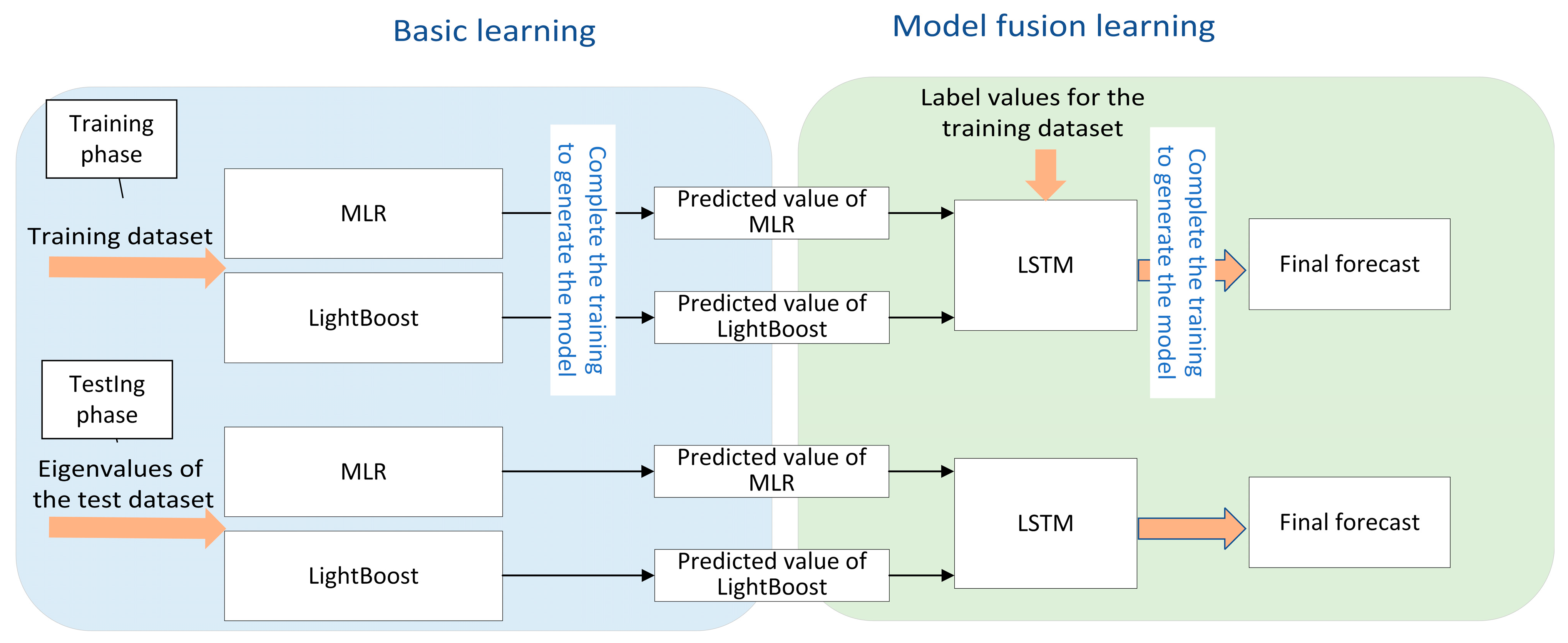
To address these issues, the following research is presented in this paper: Statistics and artificial intelligence are often distinguished, and it is generally believed that they belong to different research fields, with the former focusing on interpretable processes and the latter on optimal output results. From the perspective of data science, this paper organically combines the modeling techniques in these two fields to form a better modeling solution. In this paper, we innovatively propose a model fusion algorithm to jointly complete modeling with different and differentiated base models and model fusers according to different data sets in practical engineering applications, which not only can well-combine the unique advantages of each base model but also can adapt to different time series problems and improve the prediction accuracy and generalization ability.

The main contributions of this paper are as follows:

(1)

The contradiction of current intelligent algorithms is pointed out: the contradiction between the limited generality of intelligent algorithms and the diversity of engineering problems. A model fusion algorithm is proposed to solve this contradiction, and a theoretical analysis was performed. The algorithm can improve the generality of existing models and can be applied to different practical engineering problems in the future, providing new ideas for the research direction of intelligent algorithms;

(2)

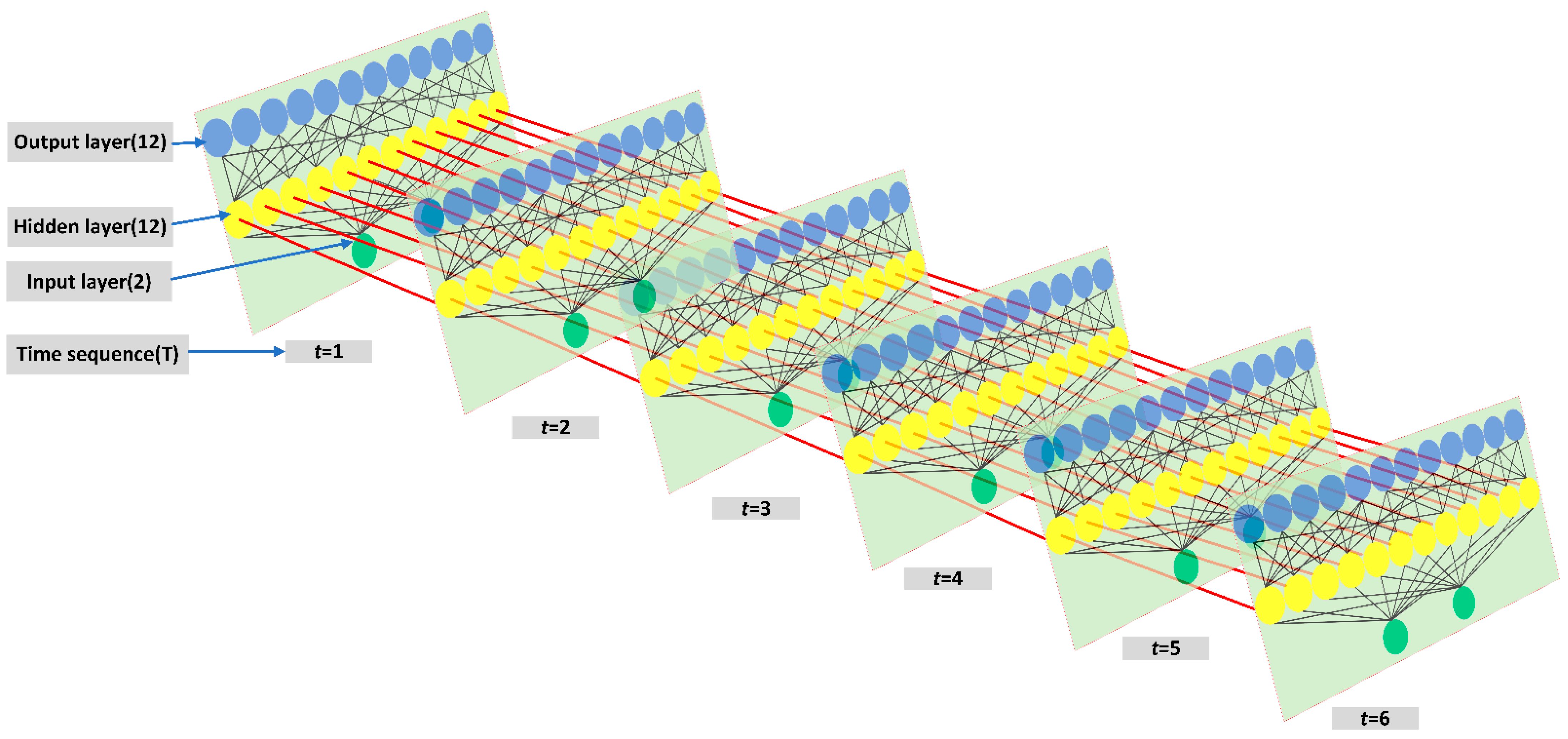
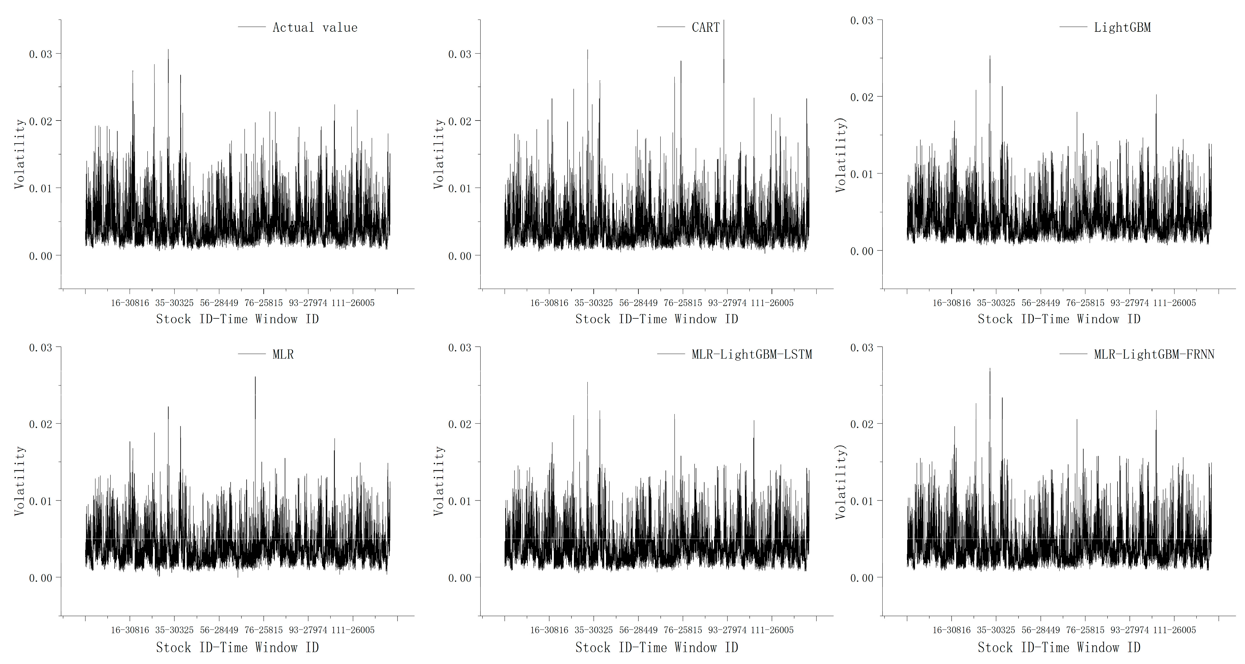
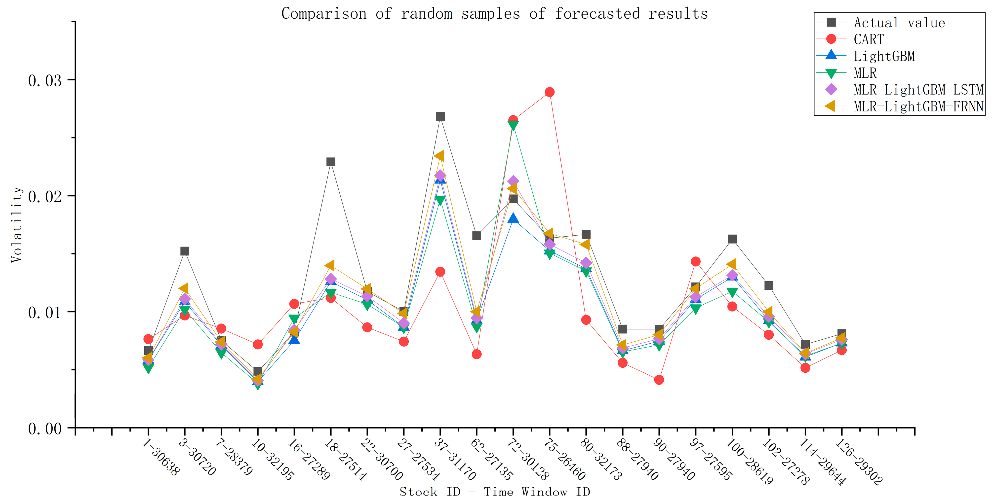
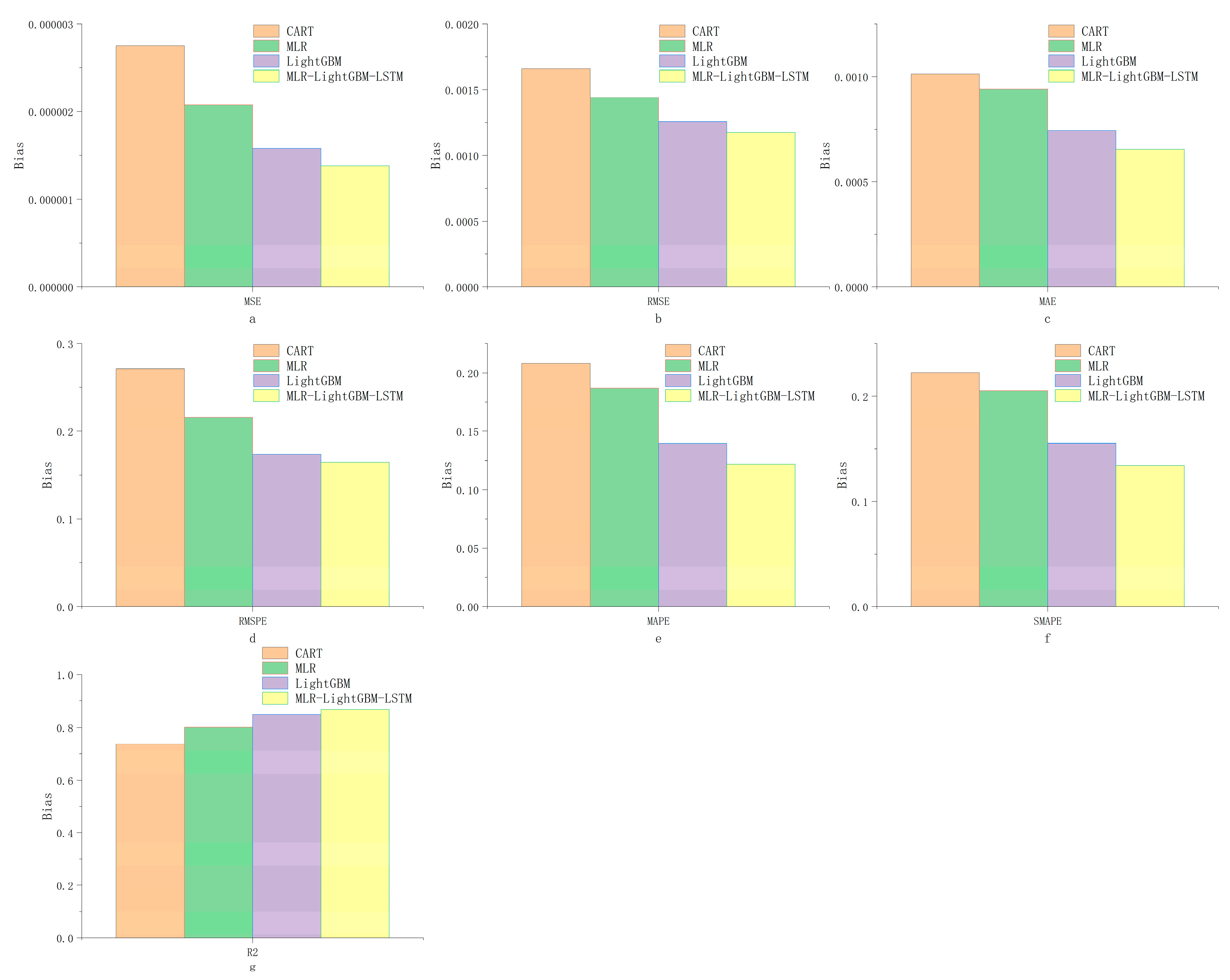
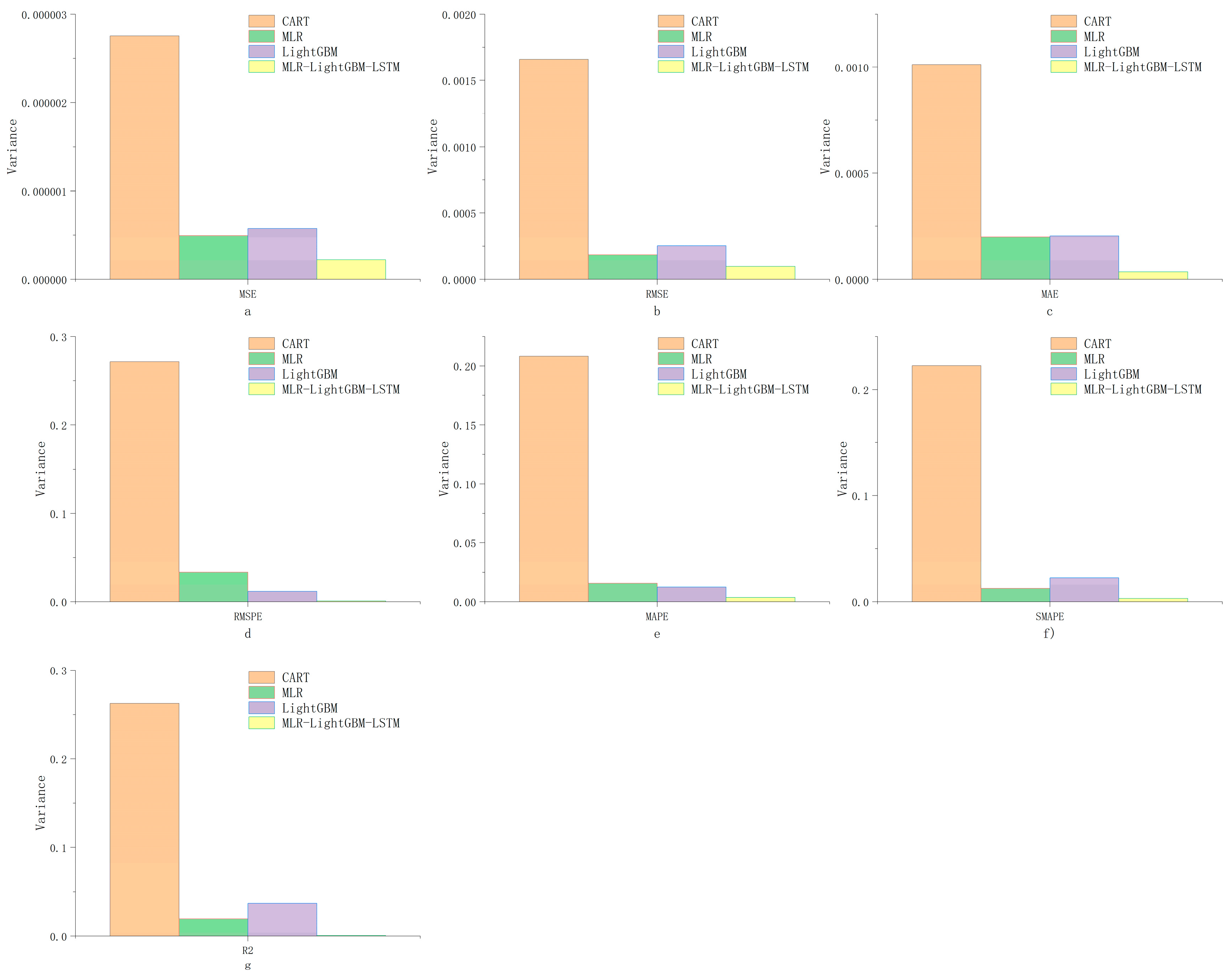
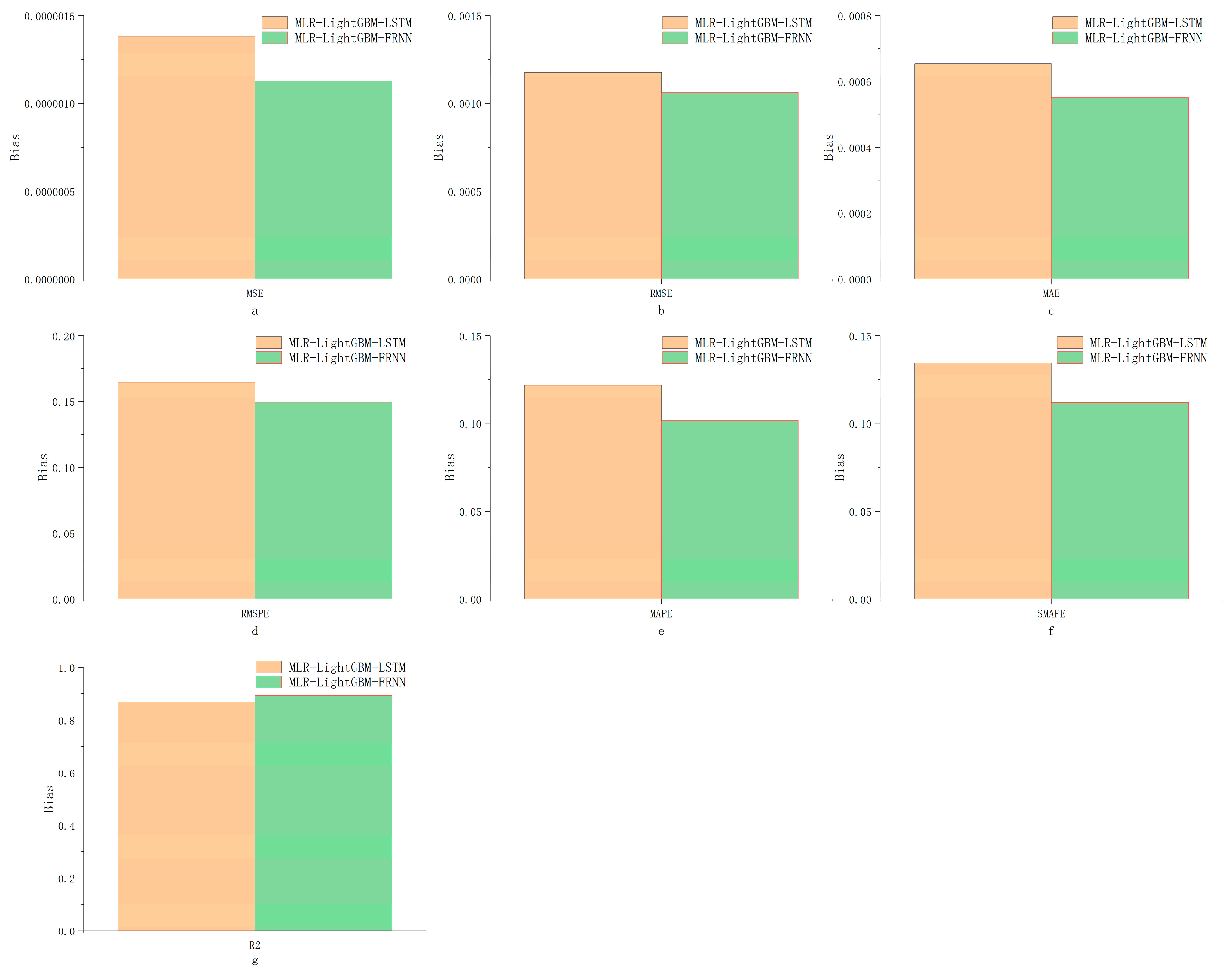
The MLR–LightGBM–LSTM and MLR–LightGBM–FRNN models are designed to predict the high-frequency volatility of 112 stocks from different industries, and the obtained prediction results have lower bias and variance than the existing mainstream models, and the model accuracy and credibility are further improved. In this paper, the same model was used to train and predict 112 stocks instead of modeling each stock separately, which is more in line with real engineering application scenarios;

(3)

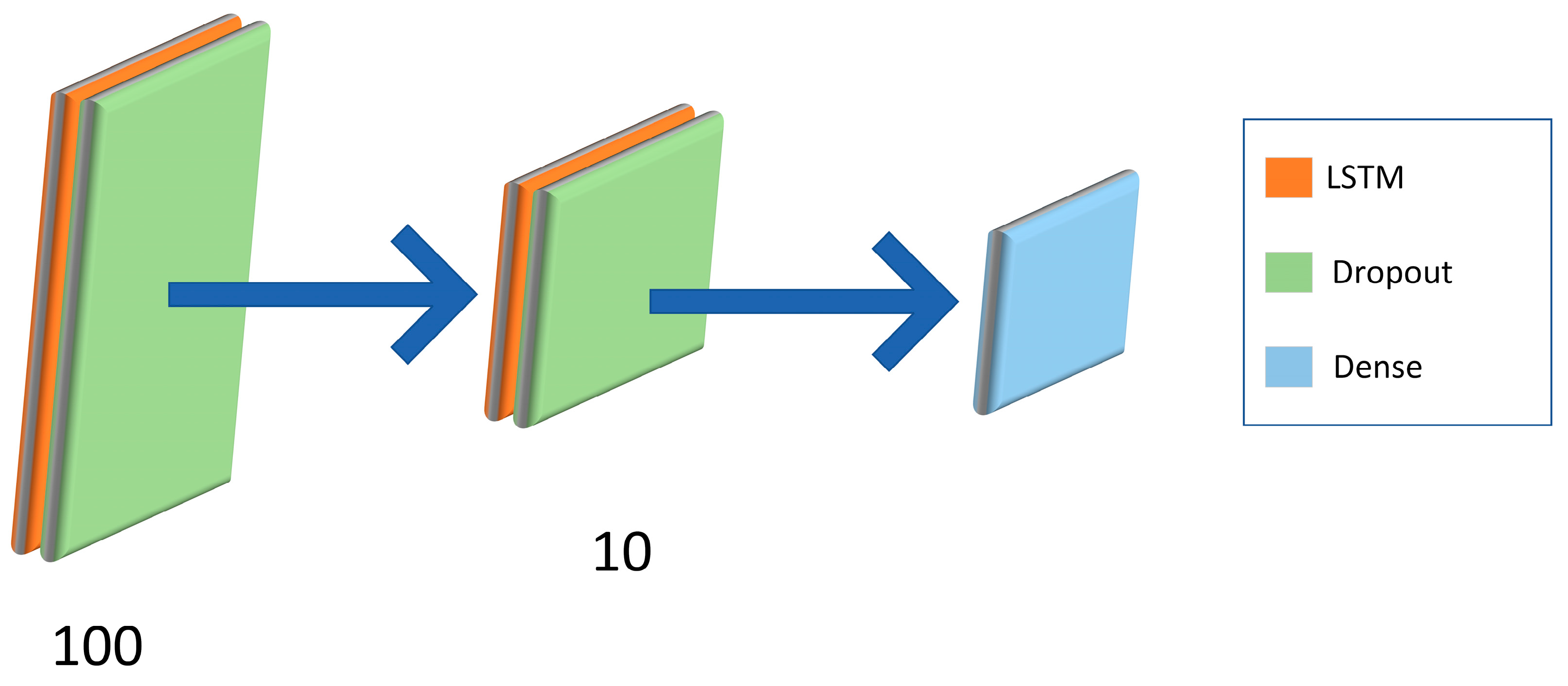
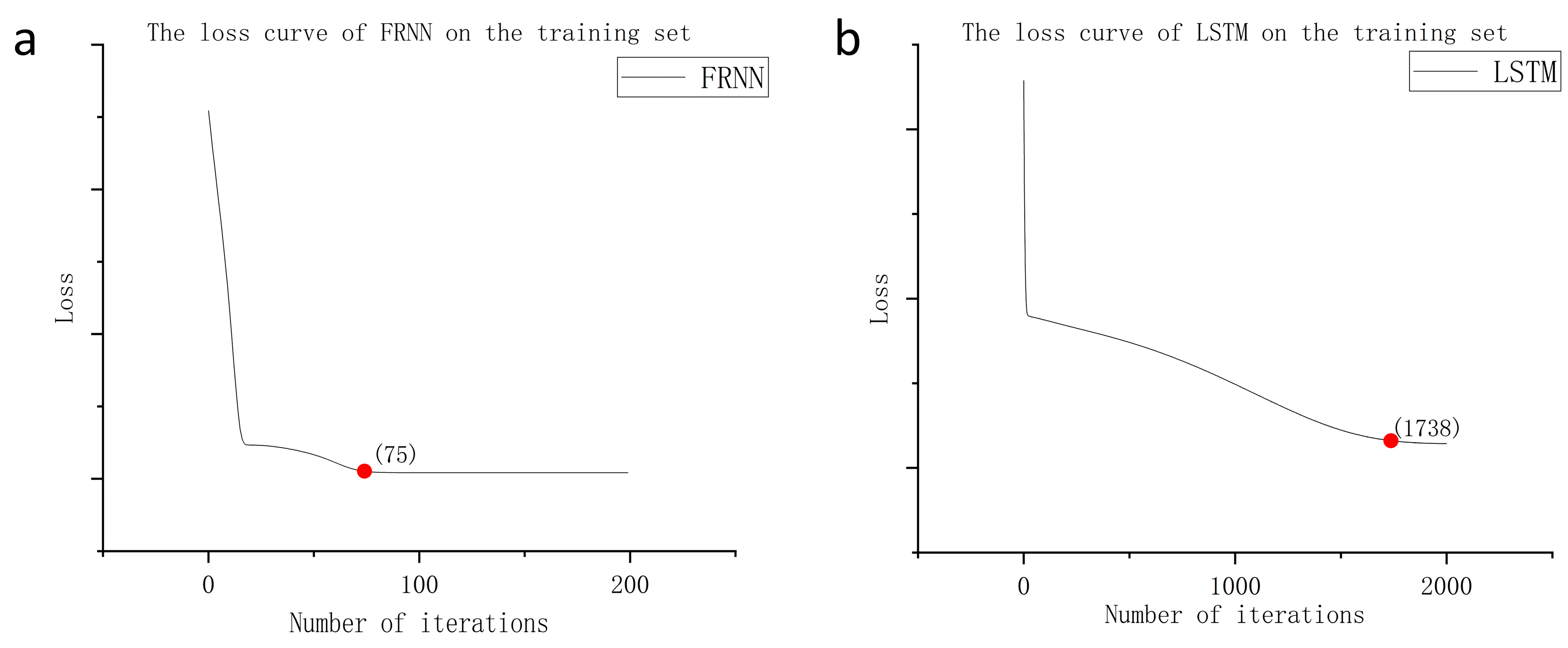
Using LSTM as a model fuser retains the advantage of predicting time series while avoiding the high expendability and instability caused by direct training with deep learning frameworks, providing a dimensionality reduction idea for deep learning modeling. In terms of error, using neural networks can quickly help the hybrid model find the balance of bias and variance, making the hybrid model simultaneously high-fitting and strongly generalizable;

(4)

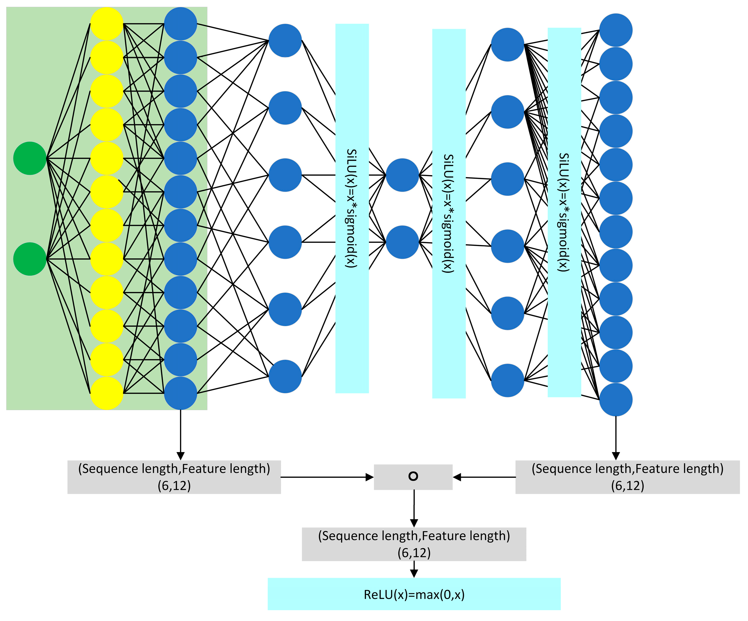
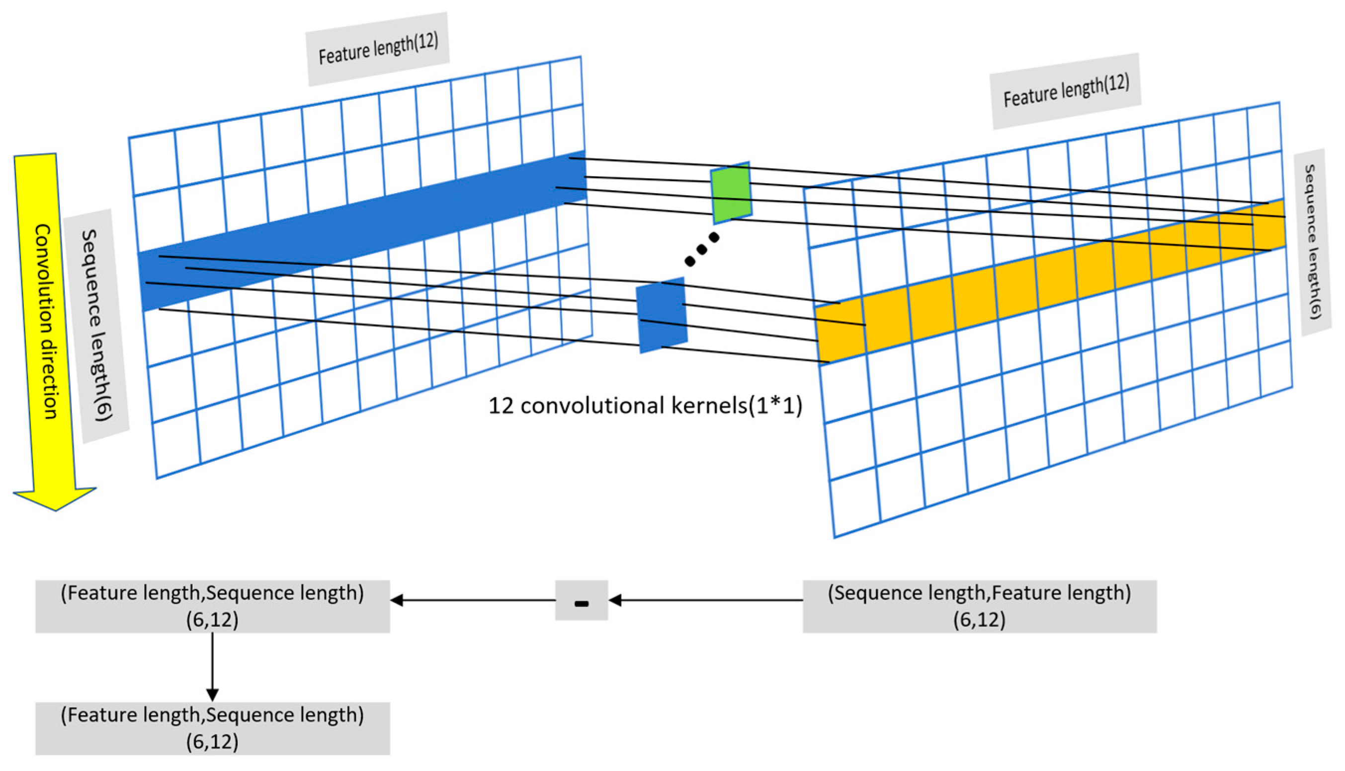
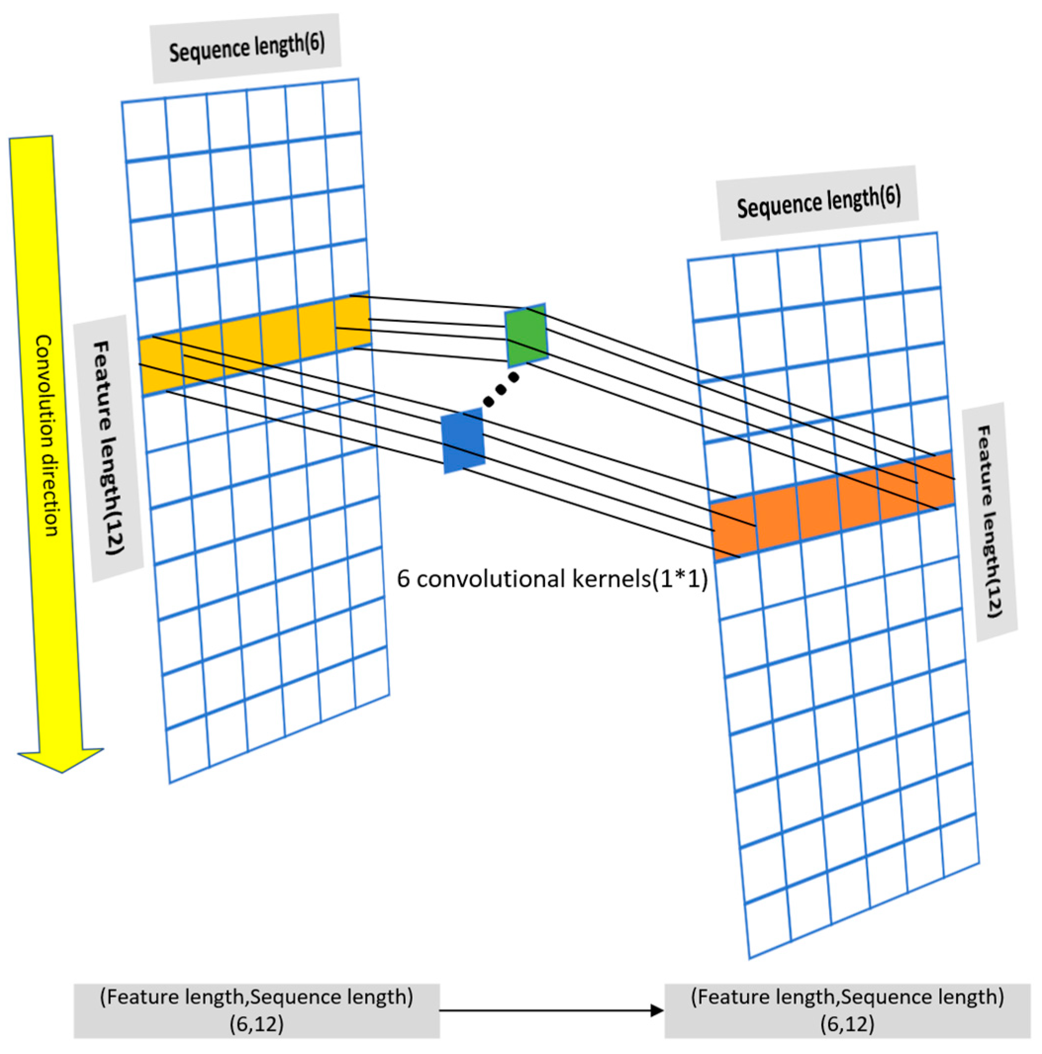
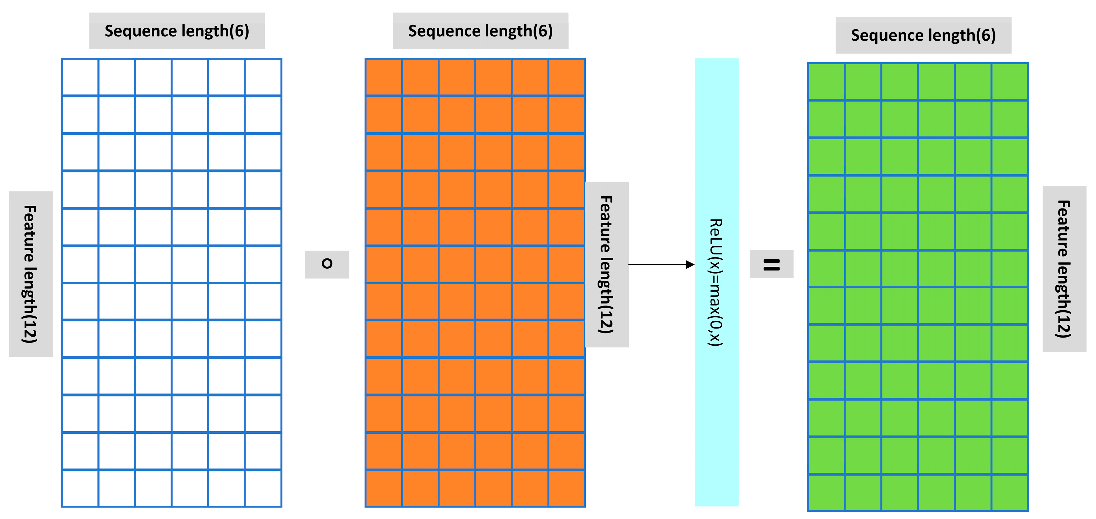
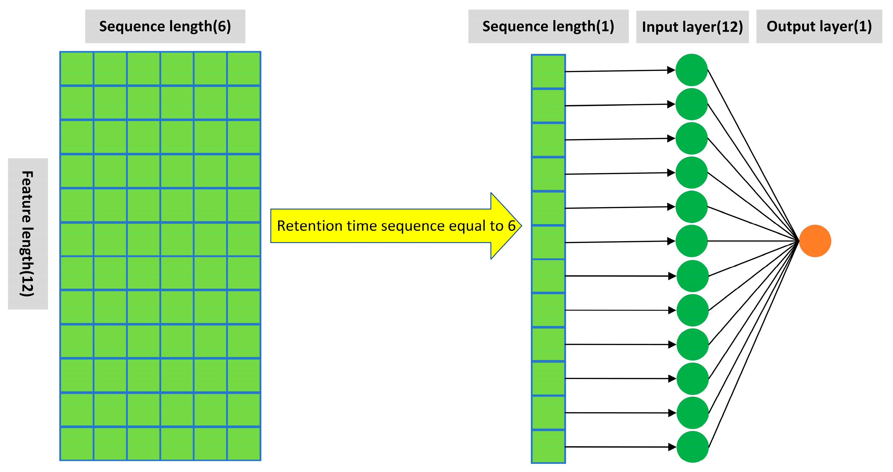
In this paper, a feature reconstruction neural network (FRNN) is innovatively proposed for datasets with few features. It can solve the problems of high error and slow fitting when existing neural networks are modeled for datasets with few features.

2. Theoretical Basis

This section briefly introduces the basic principles of MLR, CART, LightGBM, and LSTM. It also describes in detail the system architecture of the model fusion algorithm, the learning approach, the prediction process, and the designed MLR–LightGBM–LSTM model and features reconstruction neural network.

2.1. MLR (Multiple Linear Regression)

2.1.1. Mathematical Models

Linear regression is one of the most famous models in statistics. It uses regression analysis to determine the interdependent quantitative relationship between two or more variables. For a multiple regression problem with m input variables, the model takes the form of:

$$\widehat{y}={\beta }_0+{\beta }_1{x}_1+{\beta }_2{x}_2+\cdots +{\beta }_m{x}_m+\epsilon$$

(1)

$\widehat{y}$: The forecast value of the response variable;

${\beta }_0$: Unknown regression constants;

${\beta }_1,{\beta }_2,+\cdots +{\beta }_m$: Unknown model coefficients;

$x_1,x_2,+\cdots +,x_m$: The input variable;

$\epsilon$: Random error.

2.1.2. Solving the Regression Equation

The least squares method is used to solve the estimate $\stackrel{⌢}{\beta }$ of the parameter vector $\beta$ such that the random error term ε and the sum of squared residuals (SSE) are minimized. CART can be used as both a classification tree and regression tree [27]. The regression model uses an error sum-of-squares metric.

$$SSE={\displaystyle \sum _{i=1}^n{\epsilon }_i^2={\displaystyle \sum _{i=1}^n{(y_i-{\widehat{y}}_i)}^2}}$$

(2)

$$X\widehat{\beta }=Y$$

(3)

$$(X^{T}X)\widehat{\beta }=X^{T}Y$$

(4)

Solving the regression equation:

$$\widehat{Y}=\widehat{\beta }X+\epsilon$$

(5)

2.2. CART (Classification and Regression Tree)

In 1984, the decision regression tree (CART) model was proposed by Breiman et al. [28]. The CART regression tree algorithm is described as follows:

Step 1: Divide each value of each feature into two parts $D_1$ and $D_2$, calculate their error sum of squares, and use the minimum value of the error sum of squares as the division criterion to divide the optimal feature A and the optimal cut point a. The formula is as follows.

$$\underset{A,a}{\min }\left[\underset{c_1}{\min }{\displaystyle \sum }_{x_i\in D_1\left(A,a\right)}{\left(y_i-c_1\right)}^2+\underset{c_2}{\min }{\displaystyle \sum }_{x_i\in D_2\left(A,a\right)}{\left(y_i-c_2\right)}^2\right]$$

(6)

$c_1$: The mean of the output of $D_1$ samples;

$c_2$: The mean of the output of $D_2$ samples.

Step 2: Divide the data set of this node into $D_1$ and $D_2$ parts according to $A$ and $a$, and get the corresponding output values.

$$D_1\left(A,a\right)=\left(x,y\right)\in D|A\left(x\right)\le a$$

(7)

$$D_2\left(A,a\right)=\left(x,y\right)\in D|A\left(x\right)>a$$

(8)

$$c_1=average\left(y_i|x_i\in D_1\left(A,a\right)\right)$$

(9)

$$c_2=average\left(y_i|x_i\in D_2\left(A,a\right)\right)$$

(10)

Step 3. Continue to divide the two-part subset of the output according to steps one and two until the optimal combination of feature variables is found.

Step 4: Divide the input space into $D_1,D_2,\dots ,D_n$ to generate a CART regression tree, input the test set to the model, and use the mean values of the leaf nodes as the regression prediction results.

2.3. LightGBM

In 1990, Hansen and Salamon proposed that using a set of models was better than using a single model for classification, and this research gave rise to the idea of ensemble learning [29]. Ensemble learning is the combination of different base models to achieve the effect of model optimization. By “base models”, we mean some unstable models, and “unstable” means that small changes in training data can cause large changes in prediction results.

2.3.1. Bagging and Boosting

In 1996, Leo Breiman proposed the bagging integration approach (as shown in Figure 1), which combines several training subsets of the same machine learning algorithm to produce the final prediction results, thus effectively reducing the variance of the model [30].

In 1990, Schapire proposed the boosting method (as shown in Figure 2), which combines multiple weak models in a weighted way to form a strong model and iteratively optimizes it through the optimal solution of the loss function, which can effectively reduce the bias of the model [31].

2.3.2. GBDT and LightGBM

A gradient boosting decision tree (GBDT) is formed by using gradient boosting for CART. The light gradient boosting machine (LightGBM) is the best-performing GBDT implementation framework available [32,33,34].

Divide the data set into $D=\left\{\left(X_1,Y_1\right),\left(X_2,Y_2\right),\dots ,\left(X_m,Y_m\right)\right\}$. The modeling process is as follows, where h is the learner, L is the loss function, and c is the optimal output value of the leaf node.

Step 1. Initialize the decision regression tree learner.

$$h_0=\arg mi{n}_c{\displaystyle \sum }_{i=1}^{M}L\left(y_i,c\right)$$

(11)

Step 2. For the number of iterations $t=1,2,\cdots ,T$.

(a)

For each sample $i=1,2,\cdots ,M$ calculate the negative gradient (residual) for t iterations.

$$r_{ti}=-{\left[\frac{\partial L\left(y_i,f\left(x_i\right)\right)}{\partial f\left(x_i\right)}\right]}_{f\left(x\right)=f_{t-1}\left(x\right)}$$

(12)

(b)

The residuals are used as the target values of the sample data, and $\left(x_i,r_{ti}\right)$ $i=1,2,\cdots ,M$ is used as the training data of the tth tree to fit a new regression tree $h_t\left(x\right)$, which corresponds to a leaf node region of $R_{tj}\left(j=1,2,\cdots ,J\right)$, where J is the number of leaf nodes of the regression tree.

(c)

The value of the corresponding leaf node region $R_{tj}\left(j=1,2,\cdots ,J\right)$ is estimated by going to the case where the loss function is minimized.

$$r_{tj}=\arg mi{n}_c{\displaystyle \sum }_{x_i\in R_{tj}}L\left(y_i,h_{m-1}\left(x_i\right)+r\right)$$

(13)

(d)

Update the learner.

$$h_m\left(x\right)=h_{m-1}\left(x\right)+{\displaystyle \sum }_{j=1}^J{r}_{tj}I\left(x\in R_{tj}\right)$$

(14)

Step 3. Generate the final model.

$$h\left(x\right)=h_j\left(x\right)=h_0\left(x\right)+{\displaystyle \sum }_{t=1}^T{\displaystyle \sum }_{j=1}^J{r}_{tj}I\left(x\in R_{tj}\right)$$

(15)

2.4. LSTM (Long Short-Term Memory)

The introduction of artificial neural networks has produced many deep learning frameworks, the most famous being the convolutional neural network (CNN) proposed by Alexander Waibel et al. in 1987 and the recurrent neural network (RNN) proposed by Jeffrey Elman in 1990, the latter having superior performance in time series prediction [26].

2.4.1. RNN (Recurrent Neural Network)

X, S, and O in the Figure 3 denote vectors: X denotes the value of the input layer; S denotes the value of the hidden layer with the same number of nodes as the dimension of S; O denotes the value of the output layer, U is the weight matrix from the input layer to the hidden layer, and V is the weight matrix from the hidden layer to the output layer. The value S of the hidden layer of the RNN is determined by both the input X this time and the value $S_{t-1}$ of the previously hidden layer. The value of the previously hidden layer is used as the input weight W for this time.

RNN calculation formula:

$$O_t=g\left(V\ast S_t\right)$$

(16)

$$S_t=f\left(U\ast X_t+W\ast S_{t-1}\right)$$

(17)

Here, g and f are the activation functions.

However, RNNs are prone to gradient explosion and gradient disappearance during training, resulting in gradients that cannot be passed all the way through longer sequences, so RNNs cannot capture information over long distances and cannot get good time series prediction results.

2.4.2. LSTM

To overcome these drawbacks, Hochreiter and Schmidedhuber proposed the long short-term memory network (LSTM) in 1997, which is a deformation of the RNN [35]. The process of LSTM unfolding by time is shown in Figure 4.

The LSTM has three inputs: the input value $x_t$ of the network at the current moment, the output value $h_{t-1}$ of the LSTM at the previous moment, and the cell state $c_{t-1}$ at the previous moment. The LSTM has two outputs: the output value $h_t$ of the LSTM at the current moment and the cell state $c_t$ at the current moment. The LSTM introduces the concept of the gate. The LSTM uses forgetting gates and inputs to control the content of the cell state c. The output gates and the cell state together determine the output of the LSTM. The detailed calculation process of LSTM is shown in Figure 5.

The forget gate determines how much of the previous moment’s cell state is retained at the current moment.

$$f_t=\sigma \left(W_f•\left[h_{t-1},X_t\right]+b_f\right)$$

(18)

$W_f$ is the weight matrix of the forgetting gate, ${[h}_{t-1},X_t]$ denotes connecting two vectors into a longer vector, $b_f$ is the bias term of the forgetting gate, and $\sigma$ is the sigmoid function.

The input gate determines how much of the current moment’s network input is saved to the cell state $C_t$.

$$i_t=\sigma \left(W_i•\left[h_{t-1},X_t\right]+b_i\right)$$

(19)

$W_i$ is the weight matrix of the input gate, and $b_i$ is the bias term of the input gate.

The current input cell state is $C_t^{\prime }$, which is calculated based on the previous output and the current input.

$$C_t^{\prime }=tanh\left(W_c•\left[h_{t-1},X_t\right]+b_c\right)$$

(20)

$tanh$ is the activation function.

This provides the Hadamard product of the cell state $C_{t-1}$ of the previous moment and the forgotten gate $f_t$ and the Hadamard product of the cell state $C_t^{\prime }$ of the current input and the input gate $i_t$. The two products are then summed to produce the cell state $C_t$ of the current moment.

$$C_t=f_t\ast C_{t-1}+i_t\ast C_t^{\prime }$$

(21)

Below is the output gate to control how many cell states $C_t$ are output to the current output value $h_t$.

$$o_t=\sigma \left(W_0•\left[h_{t-1},X_t\right]+b_0\right)$$

(22)

The final output of the LSTM is determined by both the output gate and the cell state is as follows:

$$h_t=o_t\ast tanh\left(c_t\right)$$

(23)

We described the computational procedures of MLR, CART, LightGBM, and LSTM, which are classical regression algorithms that have also been used in time series forecasting studies or stock volatility forecasting studies, and we will use these algorithms for experimental and comparative analyses later on.

3. Methodology Innovation

This part innovatively proposes a model fusion algorithm and feature reconstruction neural network and designs the MLR–LightGBM–LSTM model and MLR–LightGBM–FRNN model.

3.1. Model Fusion Learning Algorithms

3.1.1. Algorithm Description

A large amount of the literature shows that different regression algorithms have their own advantages, disadvantages, and adaptability for different data. In this paper, we propose a model fusion meta-algorithm, using a neural network as a model fuser and a traditional statistical model or a machine learning model as a base model, and using the fuser to fuse different base models and combining the advantages of each base model to find the balance point of the bias and variance of the hybrid model. The specific implementation method is that each base model is first trained and optimized individually, and then the output of each base model is used as the input of the model fuser for training and prediction. The strategy of the model fusion learning algorithm is that different base models and model fusers can be selected for different data characteristics or business requirements, and the model fusion learning strategy has an algorithmic relative universality. When selecting a base model, we should pay attention to the diversification and difference between the models. The purpose of model fusion is to integrate the advantages of different models and avoid the shortcomings and shortcomings of a single model. The formula is described as follows:

$$O_i=f_i\left(X\right)\left(i=1,\dots ,\mathrm{n}\right)$$

(24)

$$Y=h\left(\left[O_1,\dots ,O_{\mathrm{n}}\right]\right)$$

(25)

$O_i$: The output value of the i-th base model;

$f_{\mathrm{i}}$: The i-th base model;

$Y$: The output value after model fusion;

$h$: Model fuser.

3.1.2. Theoretical Analysis

Different base models are obtained by different algorithms trained on the same dataset, and the models obtained by different algorithms have different preferences. The model fuser combines the output and target values of each base learner to complete the training and modeling, which can intuitively explain why the model fusion strategy can be successful. Learners with different preferences can label data samples differently, e.g., learner A should be able to learn some information that learner B does not have, i.e., data samples that cannot be labeled correctly by learner B may be labeled correctly by learner A and vice versa. If learners A and B have large differences, then fusing their mutual learning results may achieve better results, so it is possible that the existence of differences between different learners is a condition for the success of the model fusion algorithm.

Argumentation:

$A,B$ denote the two base learners;

$d\left(A,B\right)$ denotes the difference between learners $A$ and $B$;

$e_A$ denotes the error rate of $A$ and $e_B$ denotes the error rate of $B$.

The following inequalities exist:

$$0\le e_A\le 1$$

(26)

$$0\le e_B\le 1$$

(27)

$$0\le d\left(A,B\right)\le 1$$

(28)

There are various choices of model fusers, and the model fuser chosen in this paper is a neural network, which is used to learn a complex objective function by means of multiple simple functions and their different combinations, which can be simply expressed by the following equation:

$$Y_{com}=W_1{Y}_1\left(X\right)+W_2{Y}_2\left(X\right)+C$$

(29)

For the same data sample $X$, if the confidence level of the output $Y_1\left(X\right)$ from $A$ learner is greater than that of the output $Y_2\left(X\right)$ from $B$ learner, then the fuser will pay more attention to the output of $A$ learner when learning and vice versa. The final result $Y_{com}$ produced by the fuser will be closer to the target value.

When $d\left(A,B\right)$ is larger, the greater the labeling inconsistency between learner $A$ and learner $B$ for data sample $X$, the greater the difference between the information learned by learner $A$ and that learned by learner $B$, and the more different the information contributed by $A,B$ learners to the fuser. The fuser learns according to the principle of finding the best optimization, then the following results will be generated.

$$0\le e_{com}\le min\left(e_A,e_B\right)$$

(30)

It can be concluded from the above derivation that the difference between the base learners is a sufficient condition for the success of the model fusion strategy algorithm, i.e., as long as there is a difference between the base learners, the overall prediction accuracy can be improved by the model fusion algorithm. The different base learners show mutual support in the training process.

However, for the current study, there is no specific metric that can be used to measure the difference between the underlying models (i.e., d in Equation (28)). In this paper, we propose to portray the distance between models by quantifying their learning results during training. In this paper, two quantification formulas (31) and (32) are proposed, which are respectively applicable to normalized and non-normalized data.

$$d\left(A,B\right)=\sqrt{{\left(y_{A1}-y_{B1}\right)}^2+{\left(y_{A2}-y_{B2}\right)}^2+\cdots +{\left(y_{An}-y_{Bn}\right)}^2}$$

(31)

$$d\left(A,B\right)=1-\frac{\left|{\displaystyle {\sum }_{i=1}^n{y}_{Ai}{y}_{Bi}}\right|}{\sqrt{{\displaystyle {\sum }_{i=1}^n{y}_{Ai}^2}}\sqrt{{\displaystyle {\sum }_{i=1}^n{y}_{Bi}^2}}}$$

(32)

3.1.3. MLR–LightGBM–LSTM

At present, the mainstream modeling techniques for time series prediction problems are MLR, CART, LightGBM, and LSTM. For the specific problem of stock price return volatility prediction, a model fusion algorithm was used to design the hybrid model shown in Figure 6 and named MLR–LightGBM–LSTM, which uses LSTM as the model fuser and MLR and LightGBM as the base models. “Algorithm 1” shows a detailed description of the algorithm.

Algorithm 1. Description of MLR–LightGBM–LSTM algorithm.

MLR–LightGBM–LSTM

Input: Historical stock trading data (divided into training set and test set).

Output: The future volatility of the stock.

# Modeling

Step 1: Model the training dataset with MLR and LightBoost, respectively, and train the two learners to the best state by tuning the parameters.

Step 2: The feature values of the training set are input to the trained MLR and LightBoost, respectively, and the output results of the two models as well as the target value (true volatility) are used as the input to the LSTM for modeling, and the LSTM is trained by tuning the parameters.

#Forecast

Step 3: The feature values of the test dataset are input into MLR and LightBoost for prediction, respectively.

Step 4: The prediction results of MLR and LightBoost are used as the input of LSTM to get the final prediction.

The selection of models in MLR–LightGBM–LSTM is based on the following:

The use of MLR in statistics ensures low variance of the prediction model, LightGBM in machine learning ensures low bias of the prediction model, and two base models with large differences ensure the diversity of models and outputs.

A neural network is a kind of low-bias, high-variance model which belongs to an unstable learner. Facing high-dimensional and dynamically changing financial big data, if neural networks are used directly for prediction, there are disadvantages, such as being time-consuming, being resource-consuming, being difficult to adjust hyperparameters, having poor stability, and having poor interpretability (black box algorithm). The prediction results of the two base learners are used as inputs, and the LSTM is used as a model fuser to further fit the regression, providing a dimensionality reduction idea for deep learning, which not only combines the advantages of the two base models but also avoids the disadvantages of directly using neural networks for prediction. The advantages of autonomous adaptation, autonomous learning, fast fitting, and fast optimization search of neural networks are used to find the balance of variance and bias of the hybrid model so that the interpretability, stability, accuracy, and generalization ability of the model can reach the optimal state.

3.2. Feature Reconfiguration Neural Network(FRNN)

In terms of Taylor’s formula, any differentiable function can be approximated by a neighborhood nth-order expansion to fit the original function. The modeling principle of deep learning is similar to Taylor’s formula, so the number of features of the data directly determines the effect of deep learning; the more features of the data, the better the effect of deep learning. As of now, deep learning does not work well for modeling if the number of features is small. To address this academic problem, this paper proposes a feature reconstruction neural network, and the proposed model can get good modeling results even in the face of data sets with a small number of features.

The steps of the feature reconstruction neural network calculation are as follows:

(1)

Obtain the time series characteristics of the data. The detailed calculation process is shown in Figure 7.

$$LSTM\_Out=LSTM(Sequence\_Length,Time\_Series,Feature\_Size,Hidden\_Size)$$

(33)

(2)

Use a multilayer perceptron to perform feature compression, and then feature amplification can extract more information and avoid adding redundant features. The detailed calculation process is shown in Figure 8

$$MLP\_Out=MLP(LSTM\_Out)$$

(34)

(1)

Add attention-boosting mechanism to LSTM;

$$LSTM\_Boost=LSTM\_Out\ast MLP\_Out$$

(35)

(2)

One-dimensional convolution on time series information occurs so that the data before and after convolution have the same size and can both reduce feature redundancy and prevent feature loss. The detailed calculation process is shown in Figure 9.

$$Time\_Convolution=Conv1d\left(LSTM\_out\left(Time\_Series\right)\right)$$

(36)

(3)

Obtain information about the weights of the time series;

$$Time\_Boost=Time\_Convolution-LSTM\_out$$

(37)

(4)

One-dimensional convolution of feature information on the time series occurs so that the data before and after convolution have the same size can both reduce feature redundancy and prevent feature loss. The detailed calculation process is shown in Figure 10.

$$Feature\_Convolution=Conv1d\left(Time\_Enhance\left(Feature\_Size\right)\right)$$

(38)

(5)

The enhanced LSTM features, time series weight information, and feature weight information are fused. The detailed calculation process is shown in Figure 11.

$$Feature\_Boost=LSTM\_Boost\ast Feature\_Convolution$$

(39)

(6)

Retain the time series data at the end and output the feature information after reconstruction. The detailed calculation process is shown in Figure 12.

$$Feature\_Reconfiguration=Feature\_Boost(Time\_Series=Last)$$

(40)

We described the computational procedures of the proposed model fusion strategy and feature reconstruction neural network, and we performed experiments and comparative analysis using these algorithms.

4. Experiments and Results

Figure 13 and Algorithm 2 describe the overall idea and steps of the simulation experiment.

Algorithm 2. Simulation Description.

Stock Volatility Forecast

Input: Historical data of stock trading.

Output: The future volatility of the stock.

#Data preprocessing

Step 1. Data description: Understand the data structure of the dataset, perform data cleaning, missing value processing, data normalization, and divided into training set and test sets.

Step 2. Exploratory analysis of data: Explore the overall distribution of the dataset and prepare for the parameter setting of feature engineering and data modeling.

Step 3. Feature engineering: According to step 2, feature engineering and vector coding are performed on the dataset from the perspective of the data.

#Modeling and Training

Step 4. Modeling training and parameter tuning are performed for MLR, CART, LightGBM, LSTM, MLR–LightGBM–LSTM, and MLR–LightGBM–FRNN, respectively.

#Model Evaluation

Step 5. A variety of evaluation functions are selected to evaluate the model.

#Experimental results and analysis

Step 6. Analyze the prediction results of all models and discuss the value of model fusion algorithms and feature reconstruction neural networks.

4.1. Data Preprocessing

4.1.1. Data Description

The experimental dataset was derived from hundreds of millions of refined historical financial data provided externally by Optiver which were the trading histories of 112 stocks in different sectors over the last three years with time precision measured in seconds [36]. This dataset reflected the very rare high-frequency quantitative trading problem. The datasets were diverse and different, and conducting experiments with them together could more comprehensively and truly evaluate the effectiveness and practicality of the model. The data structure of the datasets used for the experiments is shown in

Table 1. Data Structure.

Data Name	Data Description
stock_id	Stock ID
time_id	Time window ID for stock trading
seconds_in_bucket	Specific time points (in seconds of precision)
bid_price	Expected bid price for a buy order
ask_price	Expected ask price of sell orders
bid_size	Expected number of sell orders
ask_size	Expected number of buy orders

.

The objective of the experiment was to predict future 10 min stock volatility using historical 10 min stock trading data. $S_t$ is the price of stock $S$ at time $t$. The formula for the logarithmic rate of return between t1 and t2 is:

$$r_{t1,t2}=log\left(\frac{S_{t2}}{S_{t1}}\right)$$

(41)

The logarithmic rate of return for a 10 min fixed time window can be expressed as:

$$r_t=r_{t-10min,t}$$

(42)

The square root of the sum of the squares of the log returns of all consecutive trades is the definition of volatility σ [37].

$$\mathsf{\sigma }=\sqrt{{{\displaystyle \sum }}_t^n{r}_{t-1,t}^2}$$

(43)

After normalizing the data set, the data were divided into a training set and a test set in the ratio of 9:1. To ensure the reliability of the resulting model, the data in the test set were all from the future time period compared to the training set.

4.1.2. Exploratory Analysis of Data

Figure 14 shows the data length distribution of time windows in the training set (with the stock ID of 0 as an example): a 10 min time window contains 600 s of time points, and the amount of data in the different time windows for each stock was different and normally distributed, and the amount of data in most time windows is less than 600, so the data was discontinuous. The data segment seconds_in_bucket implicitly contains information on stock activity, which can provide inspiration for feature engineering.

Figure 15 shows that the volatility distributions of both single stocks and all stocks in different time windows showed a Poisson distribution. It can provide direction for the selection of loss function in modeling.

4.1.3. Feature Engineering

Based on the exploratory analysis of the data, feature engineering was performed from the data perspective, as shown in Figure 16, with stock_id,time_id as the label. More features were generated horizontally with stock_id,time_id,target as the label and seconds_in_bucket as the target. Panel data were generated by vertical aggregation. The generated data were uniformly coded and then used for model training and prediction.

4.2. Modeling and Training

4.2.1. Experimental Environment

The simulation environment and the model training and prediction environment was Python 3.X. The experimental platform was a CPU: AMD Ryzen 9 5900HX; GPU: NVIDIA GeForce RTX 3080; 32.00 GB installed RAM.

In this paper, the same model was used to train and predict 112 stocks instead of modeling each stock separately, which is more in line with real engineering application scenarios.

The main libraries used in the experiments were the data computation libraries NumPy and Pandas, the machine learning library Scikit-learn, and the deep learning libraries PyTorch and Keras.

4.2.2. Model Parameter Setting

The following model parameters were given by trial-and-error analysis and combined with computational costs.

MLR and CART were solved optimally using least squares and MSE, respectively. The parameters of LightGBM are set as shown in

Table 2. LightGBM parameter settings.

Parameters	Value	Description
n_estimators	20,000	The maximum number of times the base model can perform boosting is 20,000.
objective	rmse	The model uses L2 as the loss function.
boosting_type	gbdt	The base learner is a gradient-boosting decision tree.
max_depth	−1	There is no maximum depth limit for the model.
learning_rate	0.01	The model learning rate is 0.01.
subsample	0.8	For each tree, 80% of the samples are randomly selected as training samples.
subsample_freq	4	Boosting is performed once every four times.
feature_fraction	0.8	For each tree, 80% of the features are selected as training samples.
lambda_l1	1	The regularization factor of L1 is 1.
lambda_l2	1	The regularization factor of L2 is 1.
random_state	66	The random number seed is 66.
early_stping_rounds	500	If the model performs 500 cycles without improvement, training is stopped.
n_fold	10	Perform 10 times crossvalidation.

.

The distance between MLR and LightGBM was calculated by Equation (31) as 0.40.

The model fuser in MLR–LightGBM–LSTM is a multilayer neural network shown in Figure 17: the first layer is an LSTM layer consisting of 100 neurons; the second layer is an LSTM layer consisting of 10 neurons, and the third layer is a dense layer. In order to prevent the overfitting phenomenon and improve the generalization ability of the fuser, the Dropout (0.2) method was used for the first two layers, i.e., the neurons were temporarily discarded according to a probability of twenty percent during the training process. The specific parameter settings are shown in

Table 3. LSTM parameter setting.

Parameters	Value	Description
loss	mean_squared_error	The loss function is the root mean square error.
optimizers	Adam (0.00001)	The training process uses Adam as the optimization algorithm with a learning rate of 0.00001.
epochs	1000	The maximum number of iterations is 1000.
validation_freq	5	Step length of 5
batch_size	30,096	The batch size is 30,096.

.

The experimental parameters of FRNN are set as shown in the legend in Section 3.2.

4.2.3. Model Evaluation

When assessing and analyzing the performance and predictive power of a model, it is necessary to use a variety of different evaluation metrics [38,39]. In order to evaluate the model comprehensively, MSE (the most common metric for prediction models), MAE (considering the outlier error), RMSE (considering the magnitude problem), RMSPE (root mean square percentage error), MAPE (considering the error proportionality problem), and SMAPE (considering the error symmetry problem) were used as evaluation metrics, and R2 was used to evaluate the goodness of fit [40,41,42,43].

$$MSE=\frac{1}{n}{\displaystyle \sum }_{t=1}^n{\left({\widehat{\sigma }}_t-{\sigma }_t\right)}^2$$

(44)

$$MAE=\frac{1}{n}{\displaystyle \sum }_{t=1}^n\left|{\widehat{\sigma }}_t-{\sigma }_t\right|$$

(45)

$$RMSE=\sqrt{\frac{1}{n}{\displaystyle \sum }_{t=1}^n{\left({\widehat{\sigma }}_t-{\sigma }_t\right)}^2}$$

(46)

$$RMSPE=\frac{1}{n}\sqrt{{{\displaystyle \sum _{t=1}^n\left(\frac{{\sigma }_t-{\widehat{\sigma }}_t}{{\sigma }_t}\right)}}^2}$$

(47)

$$MAPE=\frac{1}{n}{\displaystyle \sum _{t=1}^n\left|\frac{{\sigma }_t-{\widehat{\sigma }}_t}{{\sigma }_t}\right|}$$

(48)

$$SMAPE=\frac{1}{n}{\displaystyle \sum _{t=1}^n\frac{\left|{\widehat{\sigma }}_t-{\sigma }_t\right|}{\left({\sigma }_t+{\widehat{\sigma }}_t\right)/2}}$$

(49)

$$R^2=1-\frac{{\displaystyle {\sum }_{t=1}^n{\left({\sigma }_t-{\widehat{\sigma }}_t\right)}^2}}{{\displaystyle {\sum }_{t=1}^n{\left({\sigma }_t-{\overline{\sigma }}_t\right)}^2}}$$

(50)

${\sigma }_t$ is the real value of volatility when the time window is $t$, and ${\widehat{\sigma }}_t$ is the predicted value of volatility when the time window is $t$. Therefore, the smaller the value of the above error index, the higher the accuracy of the model prediction is, and the larger the $R^2$ is, the better the model fit is.

4.3. Empirical Results and Analysis

4.3.1. Model Fusion Algorithm

The prediction results of different models for the test set are given in Figure 18. For the sake of display and observation, the data in Figure 19 are 20 randomly selected prediction points. It is easy to find that the MLR–LightGBM–LSTM and MLR–LightGBM–FRNN models have the best prediction results both in terms of accuracy and stability. Although the volatility changes of different stocks in different sectors in different time windows are different, the prediction results of the hybrid model are closer to the true values. The volatility shown in Figure 18 is nonlinear, nonstationary, and prone to abrupt changes, so ensemble learning has become the preferred prediction algorithm, and numerous scholars have demonstrated in practice that ensemble learning is the classical algorithm with excellent performance [44,45], but the experimental results show that the model fusion algorithm can still further improve the performance of the hybrid model.

To quantify the prediction results for 112 stocks, Figure 20 and

Table 4. Model bias comparison (Based on test sets).

	MSE	RMSE	MAE	RMSPE	MAPE	SMAPE	R2
CART	0.27532 × 10−5	0.00166	0.00101	0.27141	0.20808	0.22230	0.73743
MLR	0.20759 × 10−5	0.00144	0.00094	0.21600	0.18684	0.20519	0.80203
LightGBM	0.15806 × 10−5	0.00126	0.00074	0.17369	0.13959	0.15523	0.84926
MLR–LightGBM–LSTM	0.13816 × 10−5	0.00118	0.00065	0.16472	0.12187	0.13429	0.86824

show the error results for the different models. The MSE, RMSE, MAE, MAPE, and SMAPE of MLR–LightGBM–LSTM are smaller than other models, and the R² of MLR–LightGBM–LSTM is larger than other models, indicating that the prediction accuracy and goodness of fit of MLR–LightGBM–LSTM are the best among all models.

Bias describes the difference between the predicted value and the true value and reflects the prediction accuracy of the model [46]. Variance describes the degree of difference between the model’s effect in the training set and the test set and reflects the generalization ability of the model [47]. Bias and variance are important measures of model robustness but finding the balance of bias–variance is a major challenge in regression modeling. Figure 21 shows that the bias and variance are in an inverse correlation and how the bias and variance balance of the model determines the final performance of the model.

Table 6 is obtained from the absolute value of the difference between Table 4 and

Table 5. Model bias comparison (based on the training set).

	MSE	RMSE	MAE	RMSPE	MAPE	SMAPE	R2
CART	0.00000	0.00000	0.00000	0.00000	0.00000	0.00000	1.00000
MLR	0.15826 × 10−5	0.00126	0.00074	0.18222	0.17122	0.19261	0.82133
LightGBM	0.10063 × 10−5	0.00100	0.00054	0.16199	0.12722	0.13255	0.88640
MLR–LightGBM–LSTM	0.11625 × 10−5	0.00108	0.00062	0.16374	0.11541	0.13130	0.86876

. Combining Figure 22 and

Table 6. Error Variance (obtained through Table 4 and Table 5).

	MSE	RMSE	MAE	RMSPE	MAPE	SMAPE	R2
CART	0.27532 × 10−5	0.00166	0.00101	0.27141	0.20808	0.22230	0.73743
MLR	0.04933 × 10−5	0.00018	0.00020	0.03378	0.01562	0.01258	0.01930
LightGBM	0.05743 × 10−5	0.00025	0.00021	0.01170	0.01236	0.02268	0.03714
MLR–LightGBM–LSTM	0.02191 × 10−5	0.00010	0.00004	0.00098	0.00646	0.00300	0.00052

, it can be observed that all models have biases between the training set error and the test set error, and these biases affect the confidence level of the model effects. As shown above, MLR–LightGBM–LSTM exhibits excellent model confidence while ensuring prediction accuracy. Compared with the ensemble learning algorithm, the model fusion algorithm can not only reduce the bias but also reduce the variance. Although the variance of the MLR model also presents a good advantage, the accuracy of the MLR model is not high.

4.3.2. Feature Reconfiguration Neural Network

In a MLR–LightGBM–LSTM model, the outputs of MLR and LightGBM are used as the inputs to the LSTM, and the two features are not conducive to the training of a deep learning framework. In this paper, we innovatively propose a feature reconstruction neural network to replace LSTM as a model fuser to generate a new hybrid model: MLR–LightGBM–FRNN.

The hidden layer input of an LSTM is 100 neural units, and the hidden layer input of an FRNN is 12 neural units. An FRNN has a lower model complexity and consumes fewer computational resources. Figure 23 shows the loss function curves of the two models when the learning rate and learning step are the same. It can be seen from the figure that the training speed of the FRNN is much faster than that of the LSTM.

It can be seen through Figure 24 and

Table 7. Error comparison of models.

	MSE	RMSE	MAE	RMSPE	MAPE	SMAPE	R2
MLR–LightGBM–LSTM	0.13816 × 10−5	0.00118	0.00065	0.16472	0.12187	0.13429	0.86824
MLR–LightGBM–FRNN	0.11282 × 10−5	0.00106	0.00055	0.14933	0.10161	0.11190	0.89240

that an FRNN as a model fuser has higher fit optimization and lower error rate than an LSTM deep learning framework as a model fuser.

5. Conclusions

Time series forecasting has always been a hot and difficult research topic in academic, business, and engineering fields. Quantitative trading is growing rapidly in the financial markets, and its market share is increasing while there is a huge potential space. Stock return volatility is an important measure of financial risk, and volatility forecasting is critical for investors, policymakers, and researchers. However, stock prices are often characterized by irregular fluctuations and sudden changes, making the accurate and stable prediction of volatility a difficult and challenging problem.

High-frequency trading data can be accurate to the closing price at minute/second, fully ensuring that important market information is not lost, making the volatility estimated based on high-frequency data contain richer volatility information. Realized volatility is an estimated amount of volatility constructed based on closing prices during the trading day, which, to some extent, misses market information. For investors, studying high-frequency volatility can help them better grasp trading costs in short-term trading and seek reasonable trading opportunities to obtain higher investment returns.

In this paper, the MLR–LightGBM–LSTM model and MLR–LightGBM–FRNN model were designed for the specific problem of stock volatility prediction using an LSTM and FRNN as model fusers and an MLR and LightGBM as base models. To investigate the predictive performance of the model, experiments were conducted on stock trading data of 112 different industries from the last three years. The performance of the model was measured based on evaluation metrics such as MSE, RMSE, MAE, MAPE, SMAPE, and R2. The qualitative and quantitative results show that the hybrid model outperformed the current mainstream models on all evaluation criteria, and the hybrid model has better fitting and generalization abilities. Since the stock market is a very complex and unstable system, prediction is extremely difficult if the time window is too long. The model in this paper can make a relatively accurate prediction of the volatility of the next 10 min, which is of great practical importance.

The main innovations made in this paper are as follows: (1) identification of the contradiction of current intelligent algorithms: the contradiction between the limited versatility of intelligent algorithms and the diversity of engineering problems. (2) The model fusion algorithm was proposed and theoretically analyzed, providing a research direction for the relative universality of the algorithm and a solution for the bias–variance balance. (3) The proposed model fuser provides a new direction for the application of neural networks and provides a dimensionality reduction idea for modeling deep learning. (4) Feature reconstruction neural networks can provide a better deep learning framework for modeling datasets with fewer features. (5) In this paper, the same model was used to train and predict 112 stocks instead of modeling each stock separately, which is more in line with real engineering application scenarios.

With the advent of the big data era, complex and diverse data problems have emerged in various engineering fields. In an algorithm-rich environment, we must improve the performance of modeling by combining the advantages of multiple algorithms. We hope that more outstanding scholars will join the research direction of model fusion in the future to provide more possibilities for the solution of data problems. The direction of benign development of intelligent algorithms should not just be to increase the number of new algorithms. In the future, our team will continue to explore the possibility of fusion between more machine learning algorithms; combine the advantages of different existing intelligent algorithms; explore the development of more types of model fusers; and explore more relatively universal modeling solutions to solve engineering problems.

References

1. Nateghi, R.; Aven, T. Risk Analysis in the Age of Big Data: The Promises and Pitfalls. Risk Anal. 2021, 41, 1751–1758. [Google Scholar] [CrossRef] [PubMed]
2. Bisht, D.; Singh, R.; Gehlot, A.; Akram, S.V.; Singh, A.; Montero, E.C.; Priyadarshi, N.; Twala, B. Imperative Role of Integrating Digitalization in the Firms Finance: A Technological Perspective. Electronics 2022, 11, 3252. [Google Scholar] [CrossRef]
3. Shi, Z.; Wu, Z.; Zhang, Z.; Chen, Y.; Liu, X. Learning Path Planning Algorithm Based on Career Goals and Artificial Intelligence. Int. J. Emerg. Technol. Learn. 2022, 17, 256–272. [Google Scholar] [CrossRef]
4. Al-Nefaie, A.H.; Aldhyani, T.H.H. Predicting Close Price in Emerging Saudi Stock Exchange: Time Series Models. Electronics 2022, 11, 3443. [Google Scholar] [CrossRef]
5. Daradkeh, M.K. A Hybrid Data Analytics Framework with Sentiment Convergence and Multi-Feature Fusion for Stock Trend Prediction. Electronics 2022, 11, 250. [Google Scholar] [CrossRef]
6. Jia, F.; Yang, B. Forecasting Volatility of Stock Index: Deep Learning Model with Likelihood-Based Loss Function. Complexity 2021, 2021, 5511802. [Google Scholar] [CrossRef]
7. Aouadi, A.; Arouri, M.; Roubaud, D. Information Demand and Stock Market Liquidity: International Evidence. Econ. Model. 2018, 70, 194–202. [Google Scholar] [CrossRef]
8. Osborne, M.F.M. Brownian Motion in the Stock Market. Oper. Res. 1959, 7, 145–173. [Google Scholar] [CrossRef]
9. Fama, E.F. Efficient Capital Markets: A Review of Theory and Empirical Work. J. Financ. 1970, 25, 383. [Google Scholar] [CrossRef]
10. Brown, E. A Non-Random Walk Down Wall Street. J Econ. Surv. 1999, 13, 477–478. [Google Scholar] [CrossRef]
11. Rossi, S.; Tinn, K. Rational Quantitative Trading in Efficient Markets. J. Econ. Theory 2021, 191, 105127. [Google Scholar] [CrossRef]
12. Shternshis, A.; Mazzarisi, P.; Marmi, S. Efficiency of the Moscow Stock Exchange before 2022. Entropy 2022, 24, 1184. [Google Scholar] [CrossRef] [PubMed]
13. Engle, R.F. Autoregressive Conditional Heteroscedasticity with Estimates of the Variance of United Kingdom Inflation. Econometrica 1982, 50, 987. [Google Scholar] [CrossRef]
14. Bollerslev, T. Generalized Autoregressive Conditional Heteroskedasticity. J. Econom. 1986, 31, 307–327. [Google Scholar] [CrossRef] [Green Version]
15. Awartani, B.M.A.; Corradi, V. Predicting the Volatility of the S&P-500 Stock Index via GARCH Models: The Role of Asymmetries. Int. J. Forecast. 2005, 21, 167–183. [Google Scholar] [CrossRef]
16. He, F.; Yin, L. Shocks to the Equity Capital Ratio of Financial Intermediaries and the Predictability of Stock Return Volatility. J. Forecast. 2021, 40, 945–962. [Google Scholar] [CrossRef]
17. Khaidem, L.; Saha, S.; Dey, S.R. Predicting the Direction of Stock Market Prices Using Random Forest. arXiv 2016, arXiv:1605.00003. [Google Scholar] [CrossRef]
18. Basak, S.; Kar, S.; Saha, S.; Khaidem, L.; Dey, S.R. Predicting the Direction of Stock Market Prices Using Tree-Based Classifiers. North Am. J. Econ. Financ. 2019, 47, 552–567. [Google Scholar] [CrossRef]
19. Raubitzek, S.; Neubauer, T. An Exploratory Study on the Complexity and Machine Learning Predictability of Stock Market Data. Entropy 2022, 24, 332. [Google Scholar] [CrossRef]
20. White Economic Prediction Using Neural Networks: The Case of IBM Daily Stock Returns. In Proceedings of the IEEE International Conference on Neural Networks, San Diego, CA, USA, 24–27 July 1988; IEEE: San Diego, CA, USA, 1988; Volume 2, pp. 451–458.
21. Hochreiter, S.; Schmidhuber, J. Long Short-Term Memory. Neural Comput. 1997, 9, 1735–1780. [Google Scholar] [CrossRef]
22. Maknickienė, N.; Maknickas, A. Application of Neural Network for Forecasting of Exchange Rates and Forex Trading. In Proceedings of the 7th International Scientific Conference “Business and Management 2012”, Vilnius, Lithuania, 1–2 November 2012; Selected papers. Vilnius Gediminas Technical University Publishing House Technika: Vilnius, Lithuania, 2012; pp. 122–127. [Google Scholar]
23. Chen, K.; Zhou, Y.; Dai, F. A LSTM-Based Method for Stock Returns Prediction: A Case Study of China Stock Market. In Proceedings of the 2015 IEEE International Conference on Big Data (Big Data), Washington, DC, USA, 29 October–1 November 2015; IEEE: Santa Clara, CA, USA, 2015; pp. 2823–2824. [Google Scholar]
24. Nelson, D.M.Q.; Pereira, A.C.M.; de Oliveira, R.A. Stock Market’s Price Movement Prediction with LSTM Neural Networks. In Proceedings of the 2017 International Joint Conference on Neural Networks (IJCNN), Anchorage, AK, USA, 14–19 May 2017; IEEE: Anchorage, AK, USA, 2017; pp. 1419–1426. [Google Scholar]
25. Wolpert, D.H. The Lack of A Priori Distinctions Between Learning Algorithms. Neural Comput. 1996, 8, 1341–1390. [Google Scholar] [CrossRef]
26. van der Aalst, W.; Damiani, E. Processes Meet Big Data: Connecting Data Science with Process Science. IEEE Trans. Serv. Comput. 2015, 8, 810–819. [Google Scholar] [CrossRef]
27. Tufte, E.R.; Cohen, J.; Cohen, P. Applied Multiple Regression/Correlation Analysis for the Behavioral Sciences. J. Am. Stat. Assoc. 1979, 74, 935. [Google Scholar] [CrossRef]
28. Loh, W. Classification and Regression Trees. WIREs Data Min. Knowl. Discov. 2011, 1, 14–23. [Google Scholar] [CrossRef]
29. Hansen, L.K.; Salamon, P. Neural Network Ensembles. IEEE Trans. Pattern Anal. Mach. Intell. 1990, 12, 993–1001. [Google Scholar] [CrossRef] [Green Version]
30. Breiman, L. Bagging Predictors. Mach. Learn. 1996, 24, 123–140. [Google Scholar] [CrossRef] [Green Version]
31. Schapire, R.E. The Strength of Weak Learnability. Mach. Learn. 1990, 5, 197–227. [Google Scholar] [CrossRef] [Green Version]
32. Zhong, R.; Johnson, R.; Chen, Z. Generating Pseudo Density Log from Drilling and Logging-While-Drilling Data Using Extreme Gradient Boosting (XGBoost). Int. J. Coal Geol. 2020, 220, 103416. [Google Scholar] [CrossRef]
33. Lv, J.; Wang, C.; Gao, W.; Zhao, Q. An Economic Forecasting Method Based on the LightGBM-Optimized LSTM and Time-Series Model. Comput. Intell. Neurosci. 2021, 2021, 8128879. [Google Scholar] [CrossRef]
34. Muller, F.; Schug, D.; Hallen, P.; Grahe, J.; Schulz, V. Gradient Tree Boosting-Based Positioning Method for Monolithic Scintillator Crystals in Positron Emission Tomography. IEEE Trans. Radiat. Plasma Med. Sci. 2018, 2, 411–421. [Google Scholar] [CrossRef]
35. Aldhyani, T.H.H.; Alzahrani, A. Framework for Predicting and Modeling Stock Market Prices Based on Deep Learning Algorithms. Electronics 2022, 11, 3149. [Google Scholar] [CrossRef]
36. Shi, Z. Optiver Realized Volatility Prediction[DS/OL]; Science Data Bank: Tianjin, China, 2022. [Google Scholar] [CrossRef]
37. Vlastakis, N.; Markellos, R.N. Information Demand and Stock Market Volatility. J. Bank. Financ. 2012, 36, 1808–1821. [Google Scholar] [CrossRef]
38. Lin, Z. Modelling and Forecasting the Stock Market Volatility of SSE Composite Index Using GARCH Models. Future Gener. Comput. Syst. 2018, 79, 960–972. [Google Scholar] [CrossRef]
39. Xu, Q.; Bo, Z.; Jiang, C.; Liu, Y. Does Google Search Index Really Help Predicting Stock Market Volatility? Evidence from a Modified Mixed Data Sampling Model on Volatility. Knowl.-Based Syst. 2019, 166, 170–185. [Google Scholar] [CrossRef]
40. Hacker, R.S.; Hatemi-J, A. Tests for Causality between Integrated Variables Using Asymptotic and Bootstrap Distributions: Theory and Application. Appl. Econ. 2006, 38, 1489–1500. [Google Scholar] [CrossRef]
41. Narayan, P.K.; Popp, S. A New Unit Root Test with Two Structural Breaks in Level and Slope at Unknown Time. J. Appl. Stat. 2010, 37, 1425–1438. [Google Scholar] [CrossRef]
42. Narayan, P.K.; Liu, R. A Unit Root Model for Trending Time-Series Energy Variables. Energy Econ. 2015, 50, 391–402. [Google Scholar] [CrossRef]
43. Narayan, P.K.; Liu, R.; Westerlund, J. A GARCH Model for Testing Market Efficiency. J. Int. Financ. Mark. Inst. Money 2016, 41, 121–138. [Google Scholar] [CrossRef]
44. Nabipour, M.; Nayyeri, P.; Jabani, H.; Mosavi, A.; Salwana, E. Deep Learning for Stock Market Prediction. Entropy 2020, 22, 840. [Google Scholar] [CrossRef] [PubMed]
45. Liu, Y.; Yang, C.; Huang, K.; Gui, W. Non-Ferrous Metals Price Forecasting Based on Variational Mode Decomposition and LSTM Network. Knowl.-Based Syst. 2020, 188, 105006. [Google Scholar] [CrossRef]
46. Liu, W.; Morley, B. Volatility Forecasting in the Hang Seng Index Using the GARCH Approach. Asia-Pac Financ Mark. 2009, 16, 51–63. [Google Scholar] [CrossRef]
47. Brooks, C.; Burke, S.P. Forecasting Exchange Rate Volatility Using Conditional Variance Models Selected by Information Criteria. Econ. Lett. 1998, 61, 273–278. [Google Scholar] [CrossRef]
Figure 1. Description of bagging principle.
Electronics 11 04057 g001
Figure 2. Description of boosting principle.
Electronics 11 04057 g002
Figure 3. Structure of RNN.
Electronics 11 04057 g003
Figure 4. Cell state.
Electronics 11 04057 g004
Figure 5. The calculation process of LSTM (* denotes the Hadamard product of the matrix).
Electronics 11 04057 g005
Figure 6. Architecture of MLR–LightGBM–LSTM model.
Electronics 11 04057 g006
Figure 7. LSTM_Out.
Electronics 11 04057 g007
Figure 8. MLP_Out.
Electronics 11 04057 g008
Figure 9. Time_Convolution.
Electronics 11 04057 g009
Figure 10. Festure_Convolution.
Electronics 11 04057 g010
Figure 11. Festure_Boot.
Electronics 11 04057 g011
Figure 12. Feature_Reconfiguration.
Electronics 11 04057 g012
Figure 13. Experimental steps.
Electronics 11 04057 g013
Figure 14. Data volume distribution for time windows.
Electronics 11 04057 g014
Figure 15. Volatility distribution ((a,b) denote the data distribution of single stocks and all stocks).
Electronics 11 04057 g015
Figure 16. Feature engineering.
Electronics 11 04057 g016
Figure 17. LSTM model fuser.
Electronics 11 04057 g017
Figure 18. Comparison of prediction results for the test set.
Electronics 11 04057 g018
Figure 19. Comparison of random samples of forecasted results.
Electronics 11 04057 g019
Figure 20. Model bias comparison (ag are seven different evaluation metrics).
Electronics 11 04057 g020
Figure 21. Bias–variance relationship.
Electronics 11 04057 g021
Figure 22. Model variance comparison (ag are seven different evaluation metrics).
Electronics 11 04057 g022
Figure 23. Comparison of loss function curves of FRNN and LSTM.
Electronics 11 04057 g023
Figure 24. Bias comparison (ag are seven different evaluation metrics).
Electronics 11 04057 g024