Article

Study on Price Bubbles of China’s Agricultural Commodity against the Background of Big Data

1
School of Economics and Management, Hebei Agricultural University, Baoding 071000, China
2
School of Economics and Management, Hebei University of Science and Technology, Shijiazhuang 050018, China
*
Authors to whom correspondence should be addressed.
Electronics 2022, 11(24), 4067; https://doi.org/10.3390/electronics11244067
Submission received: 28 October 2022 / Revised: 27 November 2022 / Accepted: 30 November 2022 / Published: 7 December 2022
(This article belongs to the Special Issue Artificial Intelligence Technologies and Applications)

Abstract

:
Agriculture provides a basis for social and economic development. It is therefore crucial for society and the economy to stabilize agricultural prices. Recent large increases and decreases in Chinese agricultural commodity prices have increased production risks, heightened fluctuations in the domestic agricultural supply, and impacted the stability of the global agricultural market. Meanwhile, big data technology has advanced quickly and now serves as a foundation for the investigation of time series bubbles. Identifying agricultural price bubbles is important for determining agricultural production decisions and policies that control agricultural prices. Using weekly agricultural price data from 2009 to 2021, this paper identifies agricultural price bubbles, pinpoints their time points, and examines their causes. According to our research, prices for corn, hog, green onions, pork, and ginger all have bubbles, but garlic do not. The quantity, length, time distribution, and type of bubbles differ significantly among corn, ginger, green onion, hog, and pork. The main causes for ginger and green onion price bubbles are speculation and natural disasters. Price bubbles for hog and pork are influenced by animal disease and rising costs. Conflicts between supply and demand and changes in price policy cause corn price bubbles to form. This paper advises that the government adopt various regulatory actions to stabilize agricultural prices depending on the characteristics and causes of the various types of agricultural price bubbles, it should also improve the early warning system and response mechanism for agricultural price bubbles and focus on how policies and market processes work together.

1. Introduction

The foundation of the national economic system is agriculture. As the sources of both human food and raw materials for industrial production, agricultural commodities are crucial. Among small agricultural commodities, green onion, ginger, and garlic are important seasoning ingredients. Livestock products are an important source of energy, providing essential proteins, fats, and other energy elements for humans. Among bulk agricultural commodities, food is an important material closely related to people’s lives. Meanwhile, the prices of different agricultural commodities in the market rise and fall to different degrees and the reasons are varied. In China, for example, the price of hog was only 12.15 RMB/kg in early March 2019; it rose to 39.72 RMB/kg in early November 2019, up 226.91%, then fell to 10.78 RMB/kg in early October 2021, down 72.86%. Other agricultural prices also showed large increases and decreases during the same period. China’s government has undertaken the macroeconomic control of agricultural prices [1], including the implementation of price support policies and the use of agricultural insurance. In the case of corn, for example, the government implemented a “temporary storage” policy in 2008 in Heilongjiang, Jilin, Liaoning, and Inner Mongolia to mitigate farmers’ difficulties selling grain, to stabilize the market price of corn, and to ensure food security [2]. After the implementation of the policy, corn prices rose to a high level. Thus, during the first half of 2016, the government reformed the “temporary storage” policy into a “producer subsidy” policy. This led to a sharp decline in corn prices, which began to rise again during the second half of 2020. For the purpose of developing macro-control measures, bringing down the price level and raising farmers’ incomes, it is crucial to investigate price bubbles of various agricultural commodities and their causes. Meanwhile, the rapid development of data collection and processing technology not only provides the basis for industry forecasts [3], investment analysis, and risk analysis but also improves the timeliness and science of decision-making.
Some studies use VaR models to quantify agricultural commodity price fluctuations and evaluate the risks of price fluctuations [4]. However, this method cannot identify the time points of abnormal price fluctuations. Caballero and Krishnamurthy proposed the concept of “bubble risk” [5]. Gilbert evaluated the risk of agricultural price fluctuations from a price bubble perspective to analyze the causes of international food price increases [6]. Subsequently, the “surge and fall” of agricultural price fluctuations have been examined in a number of studies using the rational bubble theory. A “price bubble” is a phenomenon in which the price of a commodity or asset deviates from its fundamental value. A commodity or asset’s initial upward price trend raises the expectations of future price increases and attracts new speculators. Speculators buy commodities or assets, not for their own use but to gain profits. When prices rise to a certain range, speculators’ expectations reverse, and commodity or asset prices sharply decline. There have been many bubbles in history that have had enormous effects, such as the Dutch “Tulip Mania” of 1636, the British “Railway Mania” of 1864–1847, the US dot-com boom in 2000, and the “Food Crisis” of 2008. The “surge and fall” of agricultural prices affects population welfare, increases the production costs and uncertainty of downstream enterprises, and adversely affects agricultural commodities and economic development [7]. Price stability, meanwhile, helps increase agricultural investment, avoid the poverty trap for low-income people, and reduce rural labor outflow [8]. Although China is a largely agricultural country, its agricultural base is weak, and factors such as natural disasters, animal diseases, speculation [9], and macro-control policies [10] may trigger agricultural price bubbles and generate adverse effects. At the same time, there are fluctuation spillover effects for agricultural prices among different countries [11,12]; it is thus necessary to study agricultural commodity price bubbles. The main purpose of this paper is to establish an analytical framework for agricultural price bubbles and provide a methodology for analyzing the different types of agricultural price bubbles. Using this analytical framework, by comparing the heterogeneity of the characteristics and causes of the different types of agricultural price bubbles, we can provide information for policymakers and a basis for stabilizing agricultural prices, as well as establish an early warning mechanism for prices.
The remainder of this paper is organized as follows. Section 2 reviews the literature on price bubbles, Section 3 describes the methods and data, and Section 4 analyzes the results and the causes of bubbles. Section 5 presents the conclusions and recommendations.

2. Literature Review

After the rational bubble theory was proposed, many researchers proposed tests to identify rational bubbles [1,13]. The main tests include the variance bound test, West’s two-step method, the unit root–cointegration test, the intrinsic bubble test, the SADF test [14], and the GSADF test [15,16]. Variance-bound tests were originally designed to assess the reasonableness of dividend discounts and their models [17,18]. Tirole suggested that the violation of the variance-bound condition could be caused by the presence of a bubble in the stock price [19]. Thus, the variance-bound test can also be used for bubble testing. The West two-step method was the first true method for bubble testing [20]. Diba and Grossman used the exponential explosive growth nature of the rational bubble to determine the presence of bubbles in asset prices by differencing dividends and asset prices [21]. Froot and Obstfeld proposed the intrinsic bubble test [22], and Phillips et al. later develop a series of tests for price bubbles [14,15,16], such as SADF and GSADF, by bridging the unit-root process and the explosive process based on the exponential explosive nature of rational bubbles. The SADF and GSADF methods have a number of advantages. First, SADF and GSADF have high testing power for periodic bubbles and can test bubbles that are relatively complex and cannot be identified by other methods. Second, SADF and GSADF can discover the process of bubble generation and bursting in real-time and capture the structural mutation point of the sequence. Finally, GSADF, as an extension of SADF, has a more flexible estimation window width, which can identify the existence of multiple bubbles within a period.
Many researchers have used SADF or GSADF to identify price bubbles and estimate bubble time points, and they can be used to test for a variety of asset bubbles. For financial assets, Phillips et al. tested the Nasdaq market price index bubble using SADF [14]. Phillips and Yu studied the beginning and end points of bond price bubbles and provided a method for establishing an early-warning mechanism [23]. However, the SADF test is good for only a single bubble. Phillips et al. proposed the GSADF method [15], using it to identify famous bubble events in the history of the S&P 500. GSADF can not only test long time-series price bubbles but also has a strong ability to identify multiple price bubbles in a series [16]. Su et al. used GSADF to test four Bitcoin bubbles, most of which occurred during the period of a significant Bitcoin rally [24]. For agricultural commodity prices, Etienne et al. found that some agricultural commodities have bubbles, but the proportion is low, and there are large differences in agricultural commodity futures price bubbles across time [25]. Li et al. found that corn and wheat price bubbles occur more frequently internationally than in China, but soybean price bubbles are more frequent in China than in the international market [1]. Using corn and soybeans as examples, Mao et al. studied price bubbles and discovered that corn typically exhibits negative bubbles, while soybeans typically exhibit positive bubbles [9]. For energy prices, Su et al. suggested that short-term bubbles in WTI crude oil spot prices are related mostly to political events or wars, and long-term bubbles are related mostly to speculative behavior [26]. Li et al. found that the EU, the US, and Asia have significant heterogeneity in the time points and duration of natural gas price bubbles [27]. Caspi et al. identified notable price bubble events in the history of WTI using GSADF to calculate the starting and ending points of bubbles [28]. Khan et al. showed that oil price bubbles usually coincide with crises, and symmetric market information helps reduce speculation and price risk [29].
Some studies have also investigated the causes of price bubbles, which can support developing regulatory measures to reduce price bubbles and stabilize market prices. Because of differences in price formation mechanisms, the causes of price bubbles for different varieties of agricultural commodities can vary widely. Etienne et al. suggested that factors such as economic growth, inventories, and export trade drive the formation of price bubbles; when the economic development level is high, inventories are low, and exports are high, positive bubbles are likely to occur, and vice versa [30]. Li et al. show that in addition to economic growth, money supply, inflation, and interest rates are important factors affecting agricultural futures markets [10]. Mao et al. analyzed the effects of exchange rates, inventories, and trade volumes on corn and soybean futures price bubbles [9]. Zhang et al., meanwhile, concluded that international soybean prices have a stronger effect on Chinese soybean prices than energy prices and are the main driver of soybean price volatility in China [12]. Caspi et al. showed that factors such as wars between major oil-producing countries, inflation, changes in supply and demand, and economic growth are important causes of oil price bubbles [28]; however, there are differences in the causes of crude oil price bubbles at different stages [29]. Li et al. argued that climate change, economic development, and changes in supply and demand are the basic factors affecting natural gas price bubbles [27]. Speculative trading can also cause bubbles in natural gas prices [31]. In general, the causes of price bubbles are multifaceted, and these factors may include macroeconomic policies, level of economic development, financial policies, supply and demand differences, international trade, and unexpected events.
Previous studies have used stock prices, agricultural prices, and energy prices to analyze the causes of price bubbles. While such work provides a basis for the present study, there are still some shortcomings. Previous studies focused mostly on the prices of bulk agricultural commodities, such as corn, wheat, and soybeans, while fewer studies investigated price bubbles in small agricultural commodities and livestock products. Few articles have developed an analytical framework from data acquisition, data analysis, and policy recommendations against the background of big data. This study’s main contributions are three parts. First, we use the GSADF method to identify different types of agricultural price bubbles in China. In order to measure different agricultural price bubble types and aid stakeholders in price bubble identification, numerous types of agricultural commodities are combined into one analytical framework in this study. Second, we examine heterogeneity in the characteristics and causes of different agricultural price bubbles to provide a basis for the formulation of policies to stabilize prices. We analyze differences among agricultural commodities in terms of the number, duration, time distribution, and properties of bubbles; analyze the causes of bubbles according to their starting and ending points; and provide a basis for formulating targeted measures. Third, we establish a complete framework for the analysis of price bubbles, which provides a reference for the study of agricultural price bubbles in other countries and regions. By using the analytical framework developed in this paper, it is possible to identify agricultural price bubbles in any country or region, providing the basis for the establishment of an early warning system.

3. Methods and Data

3.1. Theoretical Model

The weak efficient market hypothesis suggests that market price fluctuations are subject to shocks from expectations, supply, and demand while changes in market rules also affect prices [32]. Because market price fluctuations are random, wandering processes, coupled with weak efficient markets, efficient market prices reflect the fundamental value of the asset. Diba and Crossman proposed the “rational bubble” [33], wherein investors in the market can use available information to make rational judgments about the market. Investors buy overvalued assets even when asset prices rise because they expect to sell at a higher price to buyers who also expect asset prices to rise, at which point market prices deviate from their fundamental value, forming a price bubble [13,19]. Price bubbles can be identified using the capital asset pricing model. Referring to Gürkaynak’s study of price bubbles, the price of agricultural commodities in China can be expressed as
P t = ( 1 + r f ) 1 E t ( δ t + 1 + U t + 1 )
where P t denotes the Chinese agricultural price in period t , E t is the expected price in period t , δ 1 + i and U 1 + i denote the return and unforeseen portion of period t + 1 , respectively. By iterating forward, Equation (1) can be rewritten as
P t f = i = 0 ( 1 1 + r f ) i E t ( δ 1 + i + U t + i )
Equation (2) removes the bubble component of agricultural prices and describes the determinants of fundamental prices, where P t f denotes the fundamental price of agricultural commodities, and δ t + i denotes the rate of return of agricultural commodities in period t + i , i = 0 , 1 , 2 n .
B t = ( 1 + r f ) 1 E t ( B t + 1 )
Equation (3) represents sequence of random variables that can satisfy the homogeneous expectation equation. Thus, Equation (1) can be written as
P t = P t f + B t
Equation (4) contains two components. P t f represents the fundamental price of agricultural commodities, and B t denotes a bubble. If B t = 0 , the agricultural price P t is only the fundamental value; if B t 0 , the market price P t contains not only the fundamental price but also a bubble component. Because 1 + r f > 1 , if the market price contains a bubble component, the price will be characterized by significant explosive growth in the short term. Rational bubble theory verifies the existence of price bubbles and lays the foundation for testing price bubbles.

3.2. Method

3.2.1. Bubble Test Method

Rational bubble theory assumes that markets are characterized by explosive growth and that bubbles in prices can be identified by detecting explosive processes. However, traditional methods cannot detect periodically collapsing behaviors in time series [34]; thus, the SADF method is better for identifying individual bubbles in asset prices [14] and is more effective than other tests [35]. However, the GSADF method is more applicable when there are multiple bubbles in asset prices [15,16]. The prototype models for the SADF and GSADF tests are derived from the following:
P t = d T η + θ P t 1 + ε t , ε t i i d ( 0 , σ 2 )
where P t is the price series, d is a constant, and T is the sample size; η is a localization parameter that controls the size of the intercept and the drift term. In this study, we focus on the case of η > 1 / 2 , where the order of magnitude of P t is the same as that of a pure random walk. Assuming that the rolling window regression sample series starts at r 1 = 0 and ends at r 2 = r 0 + r w , r 2 [ r 0 , 1 ] , the window width is r w , and the minimum window width is r 0 ( r 0 = 0.01 + 1.8 T , T is the sample size). Equation (5) can be rewritten as
Δ P t = α r 1 , r 2 + β r 1 , r 2 P t 1 + i = 1 k φ r 1 , r 2 Δ P t i + ε t
where k is the lag order, ε t i i d ( 0 , φ r 1 , r 2 i ) , T w = [ T r w ] is the number of regression samples, and [ · ] indicates the integer part. The null hypothesis of the model is β = 1 when there is no bubble component in the price. The alternative hypothesis is β > 1 when the price contains a bubble component.
Both SADF and GSADF can be used for the examination of bubbles.
The SADF test takes the maximum value of the ADF statistic as the sup value and compares it with the critical value of the corresponding sample; a bubble exists if it is greater than the set critical value, and no bubble exists if it is less than the set critical value. The critical values are obtained from 2000 Monte Carlo simulations, and the results usually show three levels of critical values: 90%, 95%, and 99%. The starting point of the sequence is fixed at r 1 = 0 , the end point is r 2 = r 1 + r w , the window width is r w , r w = r 2 [ r 0 , 1 ] , r 0 is the minimum window width, and 1 is the maximum window size. The SADF statistic can be defined as
S A D F ( r 0 ) = sup r 2 [ r 0 , 1 ] { A D F 0 r 2 } = sup r 2 [ r 0 , 1 ] { β ^ 0 , r 2 / s e ( β ^ 0 , r 2 ) }
Equation (8) is the limiting distribution of the SADF statistic; convergence by distribution is denoted by L , and W is the standard Wiener process.
S A D F ( r 0 ) L sup r 2 [ r 0 , 1 ] r 2 0 r 2 W ( t ) d W W ( r 2 ) 0 r 2 W ( t ) d t r 2 1 / 2 [ r 2 0 r 2 W ( t ) 2 d W ( 0 r 2 W ( t ) d t ) 2 ] 1 / 2
The GSADF test calculates the maximum ADF value within a sample group by continuously changing the starting and ending points until the maximum ADF value between groups is found and compared with the critical value of the corresponding sample. A bubble exists if it is greater than the set critical value and does not exist if it is less than the set critical value. The critical values are obtained from 2000 Monte Carlo simulations, and the results usually show three levels of critical values: 90%, 95%, and 99%. The sequence start point is r 1 [ 0 , r 2 r 0 ] , the end point is r 2 [ r 0 , 1 ] , the window width is r w = r 2 r 1 , r 0 is the minimum window width, and 1 is the maximum window width. The GSADF statistic can be defined as
G S A D F ( r 0 ) = sup r 2 [ r 0 , 1 ] r 1 [ 0 , r 2 r 0 ] { A D F r 1 r 2 } = sup r 2 [ r 0 , 1 ] r 1 [ 0 , r 2 r 0 ] { β ^ r 1 , r 2 / s e ( β ^ r 1 , r 2 ) }
When the regression model contains an intercept term and the null hypothesis is a random walk, the limiting distribution of the GSADF test is as shown in Equation (10). Convergence by distribution is denoted by L , r w = r 2 r 1 , and W is the standard Wiener process. The SADF and GSADF statistics obey the standard normal distribution when the standard Wiener process is consistent with the random walk. The asymptotic critical values of the ADF statistics are calculated using Monte Carlo simulation. Assuming equal intervals for n 1 , n 2 , n N , a Gaussian random variable with a mean of 0 and a variance of 1 / N is generated for each point. Because the bootstrap technique is feasible for identifying the explosion process, it is used to calculate the limiting distributions of the SADF and GSADF statistics.
G S A D F ( r 0 ) L sup r 2 [ r 0 , 1 ] r 1 [ 0 , r 2 r 0 ] { 1 2 r w [ W ( r 2 ) 2 W ( r 1 ) 2 r w ] r 1 r 2 W ( r ) d r [ W ( r 2 ) W ( r 1 ) ] r w 1 / 2 { r w r 1 r 2 W ( r ) 2 d r [ r 1 r 2 W ( r ) d r ] 2 } 1 / 2 }
The GSADF test has a more flexible window size relative to the SADF test, which improves the test’s power by changing the starting point of the series and increasing the number of recursions. It solves the problem in which multiple bubbles cannot be detected in the SADF test. Thus, GSADF is used to test price series bubbles in this study.

3.2.2. Bubble Date Stamping

If an agricultural price bubble is verified using the GSADF test, the sequence of backward SADF (BSADF) statistics and the critical value sequence are calculated to identify the origination and termination points of the agricultural price bubble. The specific steps are as follows:
First, by fixing termination point 1 in sample T and continuously moving the position of the origination point r 1 [ 0 , r 2 r 0 ] forward, the maximum ADF statistic within the group is obtained by Equation (6); this value is the BSADF statistic at t = T . It can be expressed as
B S A D F r 2 ( r 0 ) = sup r 1 [ 0 , r 2 r 0 ] { A D F r 1 r 2 }
Second, the position of the termination point is changed, rolling r 2 forward by 1 period (fixed at T 1 ), continuously moving the position of the origination point r 1 [ 0 , r 2 r 0 ] forward. The maximum ADF statistic within the group is obtained repeatedly until r 2 = r 0 , combining the largest ADF statistics corresponding to each time point in T ( r 0 , t ) [ T r 0 , T ] into the BSADF sequence.
Third, the value of the BSADF statistic at each time point is compared with the corresponding critical value. When the BSADF value is greater than the critical value at the corresponding time point, it is recorded as the origination point of the price bubble. When it is less than the critical value at the corresponding time point, it is recorded as the termination point of the price bubble. The judgment criteria are
r ^ e = inf r 2 [ r 0 , 1 ] { r 2 : B S A D F r 2 ( r 0 ) > s c v r 2 β T }
r ^ f = inf r 2 [ r ^ e + δ log ( T ) / T , 1 ] { r 2 : B S A D F r 2 ( r 0 ) < s c v r 2 β T }
where δ log ( T ) is the minimum duration of the bubble, which can be set according to the risk tolerance, and δ is the frequency-related parameter. s c v r 2 β T is the critical value of the SADF statistic at the 100 ( 1 β T ) % significance level. The critical values of the different time points ( T ( r 0 , t ) [ T r 0 , T ] ) are obtained from 2000 Monte Carlo simulations.

3.2.3. Data Processing Procedures

With the development of computer technology, data collection and processing capabilities have been greatly improved, and big data technology is now widely used. This provides the basis for processing large amounts of data and analyzing agricultural price bubbles. However, existing studies lack a complete framework for data analysis. Referring to the research results of Ali et al. [36] and combining them with the research content of this paper, we divide the processing of Chinese agricultural price bubbles into four parts: data collection, data processing, analysis of the results, and scientific decision-making. This division is in accordance with the aforementioned research theories and methods, as well as the general process of big data processing. In Figure 1, the data processing procedure is shown.
First, for data collection, general study’s primary data sources include officially available statistics, data from web crawling, specialist databases, and survey research among other sources. The sources for a particular study must be chosen in accordance with the study’s goals and its subjects. The data used in this paper were obtained from specialist databases in accordance with the data’s accessibility and the goals of the research. Second, for data processing, the GSADF and SADF methods are used to test whether there are bubbles in agricultural prices; if there are bubbles, bubble date stamping is determined. Before processing the data, missing data should be added and redundant data must be eliminated. Third, in the analysis of the results, if there are price bubbles for a specific agricultural commodity, the bubble period, quantity, length, period, and property are identified, and a comparative analysis is performed. The bubble generation period is combined, and the causes of the price bubble on the basis of the economic climate and policies of the time are identified. Fourth, to support scientific decision-making, the results of the big data analysis can serve different participants in the market, such as buyers of agricultural commodities, makers of economic policies, and sellers of agricultural commodities. In this paper, we analyze the price bubbles of agricultural commodities to provide a basis for scientific decision-making and reduce the fluctuations of agricultural markets.

3.3. Data

To investigate whether there are bubbles in the prices of different agricultural commodities and to examine their differences, we select the weekly average prices of ginger, garlic, green onion, hog, pork, and corn as the research objects. Ginger, garlic, and green onion are small agricultural commodities that are important seasoning ingredients. Hog and pork are livestock products that provide proteins and fats for human diets. Corn has the largest production and sown area in China and is an important “grain, warp, and feed” crop. The sample period is January 2009 to December 2021. Linear interpolation is used to compensate for missing values in certain agricultural commodities. There are 674 samples for each agricultural commodity. The price data for each agricultural commodity come from the national market data in China. Prices of small agricultural commodities are obtained from national market prices published by the Ministry of Agriculture and Rural Affairs, and prices of hog, pork, and corn are the average prices of different provinces and cities in China. Data are obtained from the Wind database and processed using RStudio.
Table 1 shows the descriptive statistical analysis of each agricultural commodity. In terms of average prices, there are large differences in the prices of different agricultural commodities; pork had the highest average price and corn had the lowest average price. In terms of standard deviation, those for small agricultural commodities are higher than that of corn, showing greater fluctuation; pork is the largest, indicating that the price of livestock products is more volatile, and the market risk is high; corn is the smallest, and the fluctuation is relatively small. In terms of maxima and minima, the maximum values of ginger, hog, corn are 13.33, 4.56, and 2.02 times those of the minimum values, respectively, and the price fluctuations are drastic. In terms of skewness and kurtosis, they verify that the price fluctuations of agricultural commodities have asymmetry and “high kurtosis and fat tail” characteristics, indicating that agricultural commodities are more volatile.

4. Empirical Results

4.1. Bubbles Test for Agricultural Commodity Prices

According to Phillips et al., the SADF test is valid only for a single bubble [15]. If there are multiple bubbles in the sample period and the interval between adjacent bubbles is too large or too small, the SADF test may not identify the bubbles. Thus, the GSADF method is used in this study to determine whether bubbles exist in agricultural commodity prices. The minimum window size is set to 53 weeks ( 53 = ( 0.01 + 1.8 / 674 ) × 674 ). The SADF and GSADF statistics values and critical values for each agricultural commodity are obtained from 2000 Monte Carlo simulations; Table 2 shows the results. From the SADF test results, the SADF statistics values for ginger, garlic, and green onion prices are 0.85, 1.06, and −0.40, respectively, which are below the critical value (1.26) at the 90% level, and the null hypothesis cannot be rejected. The SADF statistics values for hog, pork, and corn prices are 7.86, 6.16, and 1.98, respectively, which are greater than the critical value (1.53) at the 95% level, thus rejecting the null hypothesis. From the GSADF test results, the GSADF statistic values for garlic is 1.94, which is below the critical value (2.03) at the 90% level, and the null hypothesis cannot be rejected. The GSADF statistics value for ginger, green onion, hog, pork, and corn are 3.27, 6.32, 10.15, 8.02, and 6.76, respectively, which are greater than the critical value (2.66) at the 99% level, thus rejecting the null hypothesis. There is no bubble in garlic prices, but there are bubbles in ginger, green onion, hog, pork, and corn prices.

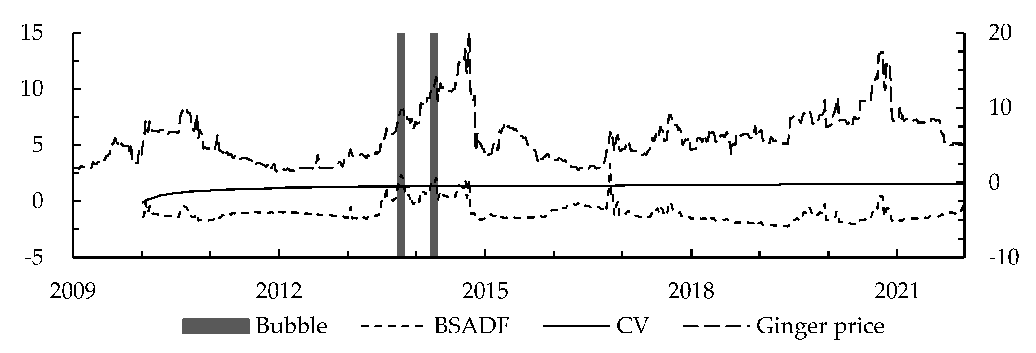
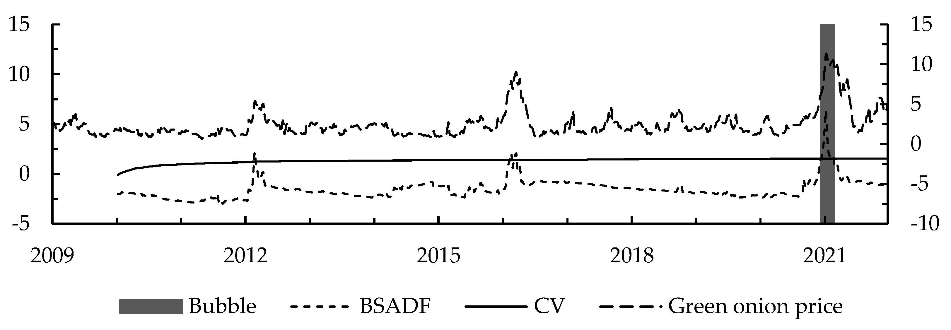
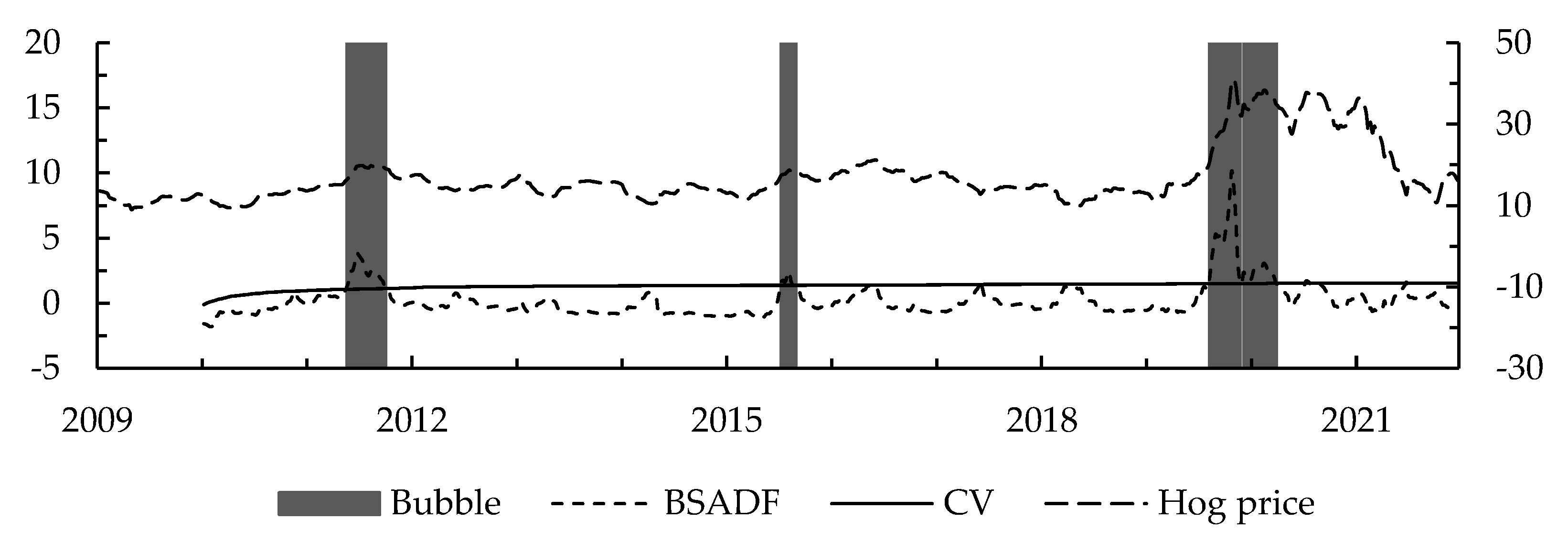
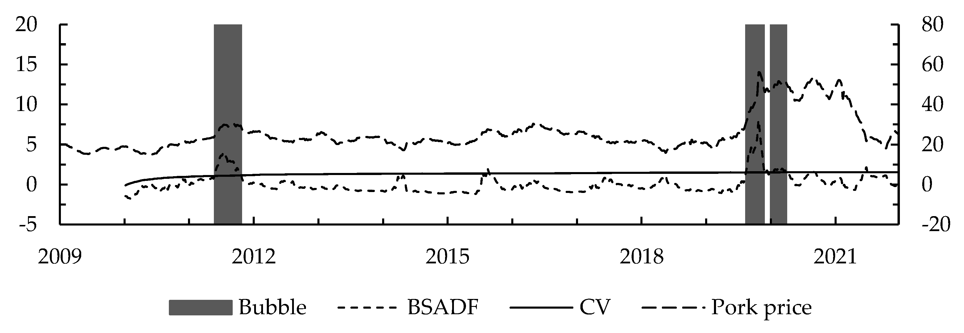
4.2. Date Stamping of Agricultural Commodity Price Bubbles

Figure 2, Figure 3, Figure 4, Figure 5 and Figure 6 shows the date stamping of agricultural commodity price bubbles. The shaded area indicates the period of the agricultural commodity price bubble, the short-dashed line indicates the BSADF statistic, the solid line indicates the critical value series at the 95% level, and the long-dashed line indicates the agricultural commodity price (right axis, RMB/kg). According to Etienne et al., a bubble is recognized when it lasts more than three days [30]. Using weekly data, we identify a bubble when the BSADF statistic exceeds the critical value at the 95% level for three consecutive weeks; we do not identify a bubble when individual BSADF values are greater than the critical value, but for less than three consecutive weeks.
The durations of small agricultural commodities bubbles are shown in Figure 2 and Figure 3. There are two bubbles in ginger prices, both of which are positive bubbles. The first bubble from 27 September 2013, to 1 November 2013, lasted five weeks, and the second bubble from 21 March 2014, to 25 April 2014, also lasted five weeks. There is one bubble for green onion prices, lasting 11 weeks from 11 December 2020, to 26 February 2021. From the analysis, it can be seen that although the number of bubbles of ginger is higher than that of green onion, the duration of individual bubbles of green onion is longer.
The durations of livestock product bubbles are shown in Figure 4 and Figure 5. There are four bubbles in hog prices, the first bubble lasted from 20 May 2011, to 7 October 2011; the second from 10 July 2015, to 4 September 2015; the third from 9 August 2019, to 29 November 2019; and the fourth from 6 December 2019, to 3 April 2020. There are three bubbles in pork prices. The first lasted from 27 May 2011, to 28 October 2011; the second from 16 August 2019, to 29 November 2019; and the third from 3 January 2020, to 3 April 2020. From the analysis, it can be seen that the number of hog price bubbles is greater than the number of pork prices, indicating that the risk of hog price volatility is higher.
The durations of corn bubbles are shown in Figure 6. Corn prices show eight bubbles, which is the largest number of observed bubbles. The first bubble lasted from 20 May 2011, to 28 October 2011; the second from 27 June 2014, to 3 October 2014; the third from 9 October 2015, to 27 November 2015; the fourth from 18 March 2016, to 24 June 2016; the fifth from 30 September 2016, to 18 November 2016; the sixth from 9 December 2016, to 12 May 2017; the seventh from 9 March 2018, to 30 March 2018; and the eighth from 19 June 2020, to 10 September 2021. From the analysis, it can be seen that the price of corn fluctuates more frequently and the risk is higher.

4.3. Characteristics of Agricultural Commodity Price Bubbles

In Table 3, Table 4 and Table 5, we can see that there are significant variances among the price bubble characteristics of the different agricultural commodities.
In terms of the number of bubbles (Table 3), green onion and ginger have one and two bubbles, respectively. This is followed by livestock products, with pork and hog having three and four bubbles, respectively. There are eight corn-price bubbles. Based on the number of bubbles, we see that small agricultural commodities have the least number of price bubbles, while bulk agricultural commodities have the highest number. The number of bubbles in the same type of agricultural commodity is relatively similar.
In terms of the total number of weeks of bubbles (Table 3), ginger and green onion prices have 10 and 11 weeks of bubbles, respectively, accounting for 1.48% and 1.63% of the total weeks (674 weeks). Hog and pork have 60 and 49 weeks of bubbles, respectively, accounting for 8.90% and 7.27% of the total weeks. Corn bubbles total 154 weeks, accounting for 22.85% of the total weeks of bubbles. This indicates that agricultural price bubbles in China mainly originate from bulk agricultural commodities. Thus, attention should be paid to their price fluctuations in the future.
In terms of the maximum single bubble duration (Table 3), corn lasts 64 weeks; hog and pork 20 and 22 weeks, respectively; and ginger and green onion 5 and 11 weeks, respectively. Different categories of agricultural commodities show significant differences, with bulk agricultural commodities, such as corn, having a longer bubble duration and small agricultural commodities having a shorter one. Therefore, the government should focus on the fluctuation of corn prices when formulating macroeconomic policies.
In terms of the properties of bubbles (Table 4), referring to Etienne’s [25] research, the bubbles can be divided into positive and negative bubbles. Ginger, green onion, hog, and pork are positive bubbles; corn prices are positive bubbles for 104 weeks, or 67.53%, and negative bubbles for 50 weeks, or 32.47%. The total number of weeks of positive bubbles for the five agricultural commodities is 234, accounting for 82%. The total number of weeks of negative bubbles is 50, accounting for only 18%. From Table 4, we can also determine the minimum and the maximum price changes during bubbles.
In terms of the temporal distribution of bubbles (Table 5), the number of bubble weeks in 2011, 2019, 2020, and 2021 are 65, 35, 55, and 44, respectively, accounting for 22.89%, 12.32%, 19.37%, and 15.49% of the total bubble periods of the five agricultural commodities; these are all above 10%. In 2014, 2015, 2016, and 2017, there are 19, 15, 25, and 18 bubble weeks, respectively, accounting for 6.69%, 5.28%, 8.80%, and 6.34% of the total bubble period among the five agricultural commodities. The remaining years are below 5%.

4.4. Causes of Agricultural Commodity Price Bubbles

Agricultural commodity price bubbles are influenced by various factors. However, different agricultural commodity bubbles are affected by different factors. In this study, we analyze the causes of different agricultural price bubbles according to the time point when the bubble is generated, taking into account the economic environment, macro policies, and unexpected events in the bubble period [37].

4.4.1. Causes of Small Agricultural Commodity Price Bubbles

The price bubbles for ginger in 2013 and 2014 were caused mainly by speculation by intermediaries and a reduction in ginger production [38]. Ginger has good storage capacity and can be stored for a long time. Thus, intermediaries buy ginger in large quantities at low prices to control the supply while reducing the number of shipments, causing price increases. Meanwhile, affected by the previous price downturn, ginger production dropped significantly in 2013, while the demand for ginger remained strong. Thus, the contradiction between supply and demand was prominent, pushing up the price of ginger and forming a price bubble. The bubble in green onion prices was caused mainly by natural disasters and high demand. In 2020, China suffered from continuous rains, with a national average precipitation of 686 mm, 10% more than normal. The area affected by flooding increased to 7190 thousand ha, 509.6 thousand ha more than in 2019. The disaster caused a reduction in green onion production and a decrease in market supply. From the end of 2020 to the beginning of 2021, market demand increased because of holidays such as the Spring Festival, which pushed up green onion prices and, thus, formed a price bubble. Therefore, supply and demand fundamentals and speculative factors are the main causes of small agricultural price bubbles.

4.4.2. Causes of Livestock Product Price Bubbles

Hog and pork have some similar causes for bubbles. The first bubble for hog and pork was influenced mainly by rising costs and loose monetary policy. Hog farming uses corn mainly as feed, and an increase in corn prices push up hog farming costs, which, in turn, affects pork prices. After the 2008 financial crisis, the Chinese government implemented a loose monetary policy, which led to the formation of price bubbles [39]. The second hog bubble was influenced mainly by a decline in breeding sow stock and hog slaughter. In January 2015, the number of breeding sows was 41.9 million, which dropped to 37.98 million in December. The number of hogs slaughtered in 2015 was 70.825 million, down 26.854 million from 2014 (Wind database). The decline in the stock of breeding sows and the slaughter of hogs decreased the number of hogs supplied in the market, pushing up prices and forming a bubble. However, the duration of the hog bubble was short, the transmission to pork prices was not obvious, and no bubble was formed in pork prices. The third and fourth price bubbles for hog and the second and third bubbles for pork occurred in the second half of 2019 and the first half of 2020, respectively. This was related mainly to African swine fever and the rising cost of farming [40]. In 2019, African swine fever led to a large number of deaths among breeding sows and hogs, reducing the stock of breeding sows and hogs slaughtered. The substantial increase in corn prices at this stage was also an important factor pushing up the price of hog and pork. According to the above analysis, the reasons for livestock product price bubbles are rising costs, animal diseases, monetary policy, and the fundamentals of supply and demand.

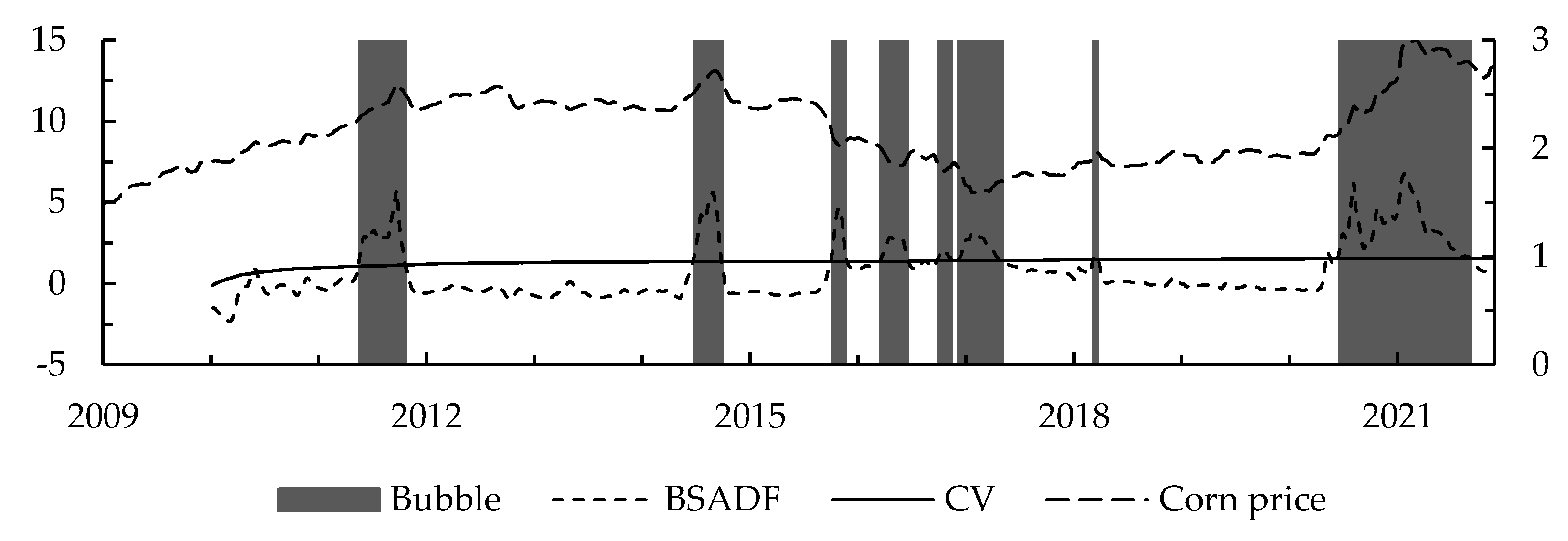
4.4.3. Causes of Corn Price Bubbles

Corn prices have experienced multiple bubble processes in recent years. The causes are not all the same, but they are closely related to government regulation [1,38]. The first and second bubbles were affected by the temporary storage policy. When the state grain reserve and other institutions were open to buying corn based on the temporary storage price and farmers had better expectations of the market, this caused corn prices to continue to rise, and bubbles were formed. The third, fourth, fifth, and sixth bubbles are related to the market-oriented reform of the temporary storage policy, and these four bubbles are all negative. With the implementation of the temporary storage policy, China’s domestic corn stock was high, and the government’s financial burden increased. To reduce stocks and alleviate the government’s financial pressure, the government adjusted the temporary storage price in the second half of 2015, lowering it to 2 RMB/kg from the 2014 levels of 2.22–2.26 RMB/kg, and market expectations fell. In the first half of 2016, the government changed the temporary storage policy to a producer subsidy policy, and market expectations fell further, driving the third, fourth, fifth, and sixth negative bubbles. The seventh and eighth bubbles are influenced mainly by corn supply and demand. This supply-side structural reform contributed to a decline in corn stock. Hog and other breeding industries recovered, and the market demand for corn was strong, the supply of corn was less than the demand, and prices continued to climb, driving the formation of the bubbles. According to the above analysis, macro-control policies, and supply and demand fundamentals are the main drivers of corn price bubbles.

4.5. Discussion of Empirical Results

Among small agricultural commodities, there are generally price bubbles for ginger and green onions, but not for garlic. According to Zhang’s study [38], there are bubbles in garlic but not in green onions, which may be related to the data selection and critical value selection (95% in this paper, whereas Zhang et al. selected 90%). Natural disasters can reduce crop yield, which may affect the supply–demand mismatch and result in the formation of a bubble, but price changes for small agricultural commodities are attributed primarily to market speculation. Therefore, the goal of developing future policies should be to control market speculation. According to our the results, it can be seen that the time point of the price significant growth or reduction for ginger and green onions is consistent with their bubble periods.
The time point of the price bubbles for hog and pork among livestock products is comparable, suggesting a connection between upstream and downstream product bubbles in the industry chain. Upstream agricultural price bubbles may also be communicated to downstream agricultural products. Looking at the root causes of bubble development, monetary policy, supply and demand dynamics, and animal diseases are significant factors, but the influence brought on by African swine fever is larger. For instance, the spike in pork prices in 2019 is directly tied to African swine fever [40]. The price alert system should take on a commensurate role. From the results, the time point of the price significant growth or reduction in hog and pork is consistent with their bubble periods.
Corn spot price bubbles are more frequent and endure longer than those for other small agricultural and livestock products. While less research has been conducted on spot prices and more on corn futures prices, the causes of price bubbles are commonly the same, and can include the mismatch between institutions supporting supply and demand or price support policy reform [1,10]. The government should pay attention to the early warnings and macro-control of the corn price bubble, because corn holds a fundamental role in the entire agricultural market. From the results, the time point of price significant growth or reduction in corn is consistent with its bubble periods.

5. Conclusions and Recommendations

Considering weekly price data for agricultural commodities in China from January 2009 to December 2021, we examine the date stamping and characteristics of different agricultural commodities’ price bubbles and analyze their causes. The development of big data technology provides analytical tools and data for the testing of agricultural price bubbles. The findings are as follows: (1) Using the GSADF test, we tested the price bubbles of different agricultural commodities. The test results showed that most agricultural commodities have bubbles in their prices. Bubbles exist in five agricultural commodities (i.e., ginger, green onion, hog, pork, and corn), while no bubbles exist for garlic. (2) There are significant differences in the characteristics of price bubbles for different agricultural commodities. In this paper, we analyzed the number of bubbles, bubble weeks, maximum single bubble duration, bubble properties, and bubble temporal distribution. From the results, we see that corn price bubbles are the most likely to arise; bubbles among prices of similar agricultural commodities show a strong correlation, such as hog and pork; small agricultural commodity price bubbles are less likely, and are mostly related to speculation. (3) Agricultural price bubbles have different causes. Small agricultural commodity bubbles are affected mainly by factors such as speculation and natural disasters. Livestock product bubbles are related mostly to production costs and major animal diseases. Price bubbles for corn are affected by factors such as price support policies and contradictions between supply and demand.
On the basis of the conclusions, this paper makes the following recommendations. First, the government must take into account the characteristics and causes of various agricultural price bubbles while regulating the agricultural market. For the prices of small agricultural commodities, it is important to focus on the regulation of speculators to lessen the large fluctuations brought on by speculation; for the prices of livestock products, it is important to increase medical assistance and prevent major animal diseases to lessen the price bubbles brought on by massive animal deaths; for the prices of corn, attention should be paid to the supply and demand relationship in the market to avoid the price bubbles caused by the imbalance between the supply and demand structure. Second, the early warning system and response mechanism for agricultural price bubbles must be improved. A real-time monitoring system for agricultural prices should issue a bubble alert when the price bubble surpasses a predefined target, and the regulatory authority should initiate an alert reaction mechanism. In the meantime, the early warning system could be improved on the basis of big data calculations to increase the precision and promptness of agricultural price warnings. Third, attention must be paid to how market processes and policy interactions are coordinated. Government spending is one of the key components of public policy [41], but excessive government spending (such as the temporary storage policy) hinders market functioning, sharply alters the market price of agricultural products, and hastens the formation of bubbles. As a result, coordination between policy and market mechanisms [42] should be prioritized to ultimately stabilize agricultural prices and increase farmers’ income.

Author Contributions

J.W. (Jiayue Wang) contributed to the methodology, writing—original draft, and formal analysis; K.M. contributed to data curation and software; L.Z. and J.W. (Jianzhong Wang) contributed to the conceptualization and writing—review and editing. All authors have read and agreed to the published version of the manuscript.

Funding

This research received no external funding.

Data Availability Statement

Data are available upon request.

Conflicts of Interest

The authors declare no conflict of interest.

References

  1. Li, J.; Li, C.; Chavas, J.P. Food price bubbles and government intervention: Is China different? Can. J. Agric. Econ. 2017, 65, 135–157. [Google Scholar] [CrossRef]
  2. Qian, J.; Ito, S.; Zhao, Z. The effect of price support policies on food security and farmers’ income in China. Aust. J. Agr. Resour. Ec. 2020, 64, 1328–1349. [Google Scholar] [CrossRef]
  3. Javed Awan, M.; Mohd Rahim, M.S.; Nobanee, H.; Munawar, A.; Yasin, A.; Zain, A.M. Social media and stock market prediction: A big data approach. Comput. Mater. Contin. 2021, 67, 2569–2583. [Google Scholar] [CrossRef]
  4. Giot, P. The information content of implied volatility in agricultural commodity markets. J. Futur. Mark. Futur. Options Other Deriv. Prod. 2003, 23, 441–454. [Google Scholar] [CrossRef]
  5. Caballero, R.J.; Krishnamurthy, A. Bubbles and capital flow volatility: Causes and risk management. J. Monet. Econ. 2006, 53, 35–53. [Google Scholar] [CrossRef] [Green Version]
  6. Gilbert, C.L. How to understand high food prices. J. Agr. Econ. 2010, 61, 398–425. [Google Scholar] [CrossRef]
  7. Xie, H.; Wang, B. An empirical analysis of the impact of agricultural product price fluctuations on China’s grain yield. Sustainability 2017, 9, 906. [Google Scholar] [CrossRef] [Green Version]
  8. Lundberg, C.; Abman, R. Maize price volatility and deforestation. Am. J. Agr. Econ. 2022, 104, 693–716. [Google Scholar] [CrossRef]
  9. Mao, Q.; Ren, Y.; Loy, J. Price bubbles in agricultural commodity markets and contributing factors: Evidence for corn and soybeans in China. China Agr. Econ. Rev. 2021, 13, 91–122. [Google Scholar] [CrossRef]
  10. Li, J.; Chavas, J.P.; Etienne, X.L.; Li, C. Commodity price bubbles and macroeconomics: Evidence from the Chinese agricultural markets. Agr. Econ. 2017, 48, 755–768. [Google Scholar] [CrossRef]
  11. Chen, Q.; Weng, X. Information flows between the US and China’s agricultural commodity futures markets-based on VAR-BEKK-Skew-t model. Emerg. Mark. Financ. Trade 2018, 54, 71–87. [Google Scholar] [CrossRef]
  12. Zhang, Y.; Li, C.; Xu, Y.; Li, J. An attribution analysis of soybean price volatility in China: Global market connectedness or energy market transmission? Int. Food Agribus. Man. 2021, 24, 15–25. [Google Scholar] [CrossRef]
  13. Gürkaynak, R.S. Econometric tests of asset price bubbles: Taking stock. J. Econ. Surv. 2008, 22, 166–186. [Google Scholar] [CrossRef]
  14. Phillips, P.C.; Wu, Y.; Yu, J. Explosive behavior in the 1990s Nasdaq: When did exuberance escalate asset values? Int. Econ. Rev. 2011, 52, 201–226. [Google Scholar] [CrossRef] [Green Version]
  15. Phillips, P.C.; Shi, S.; Yu, J. Testing for multiple bubbles: Historical episodes of exuberance and collapse in the S&P 500. Int. Econ. Rev. 2015, 56, 1043–1078. [Google Scholar]
  16. Phillips, P.C.; Shi, S.; Yu, J. Testing for multiple bubbles: Limit theory of real-time detectors. Int. Econ. Rev. 2015, 56, 1079–1134. [Google Scholar] [CrossRef] [Green Version]
  17. Shiller, R. Do stock prices move too much to be justified by subsequent changes in dividends? Am. Econ. Rev. 1981, 71, 421–736. [Google Scholar]
  18. Leroy, S.F.; Porter, R.D. The present-value relation: Tests based on implied variance bounds. Econometrica 1981, 49, 555–574. [Google Scholar] [CrossRef]
  19. Tirole, J. Asset bubbles and overlapping generations. Econometrica 1985, 53, 1499–1528. [Google Scholar] [CrossRef]
  20. West, K.D. A specification test for speculative bubbles. Q. J. Econ. 1987, 102, 553–580. [Google Scholar] [CrossRef] [Green Version]
  21. Diba, B.T.; Grossman, H.I. Explosive rational bubbles in stock prices? Am. Econ. Rev. 1988, 78, 520–530. [Google Scholar]
  22. Froot, K.A.; Obstfeld, M. Intrinsic Bubbles: The Case of Stock Prices. Am. Econ. Rev. 1991, 81, 1189–1214. [Google Scholar]
  23. Phillips, P.C.B.; Yu, J. Dating the timeline of financial bubbles during the subprime crisis. Quant. Econ. 2011, 2, 455–491. [Google Scholar] [CrossRef] [Green Version]
  24. Su, C.; Li, Z.; Tao, R.; Si, D. Testing for multiple bubbles in bitcoin markets: A generalized sup ADF test. Jpn. World Econ. 2018, 46, 56–63. [Google Scholar] [CrossRef]
  25. Etienne, X.L.; Irwin, S.H.; Garcia, P. Bubbles in food commodity markets: Four decades of evidence. J. Int. Money Financ. 2014, 42, 129–155. [Google Scholar] [CrossRef] [Green Version]
  26. Su, C.; Li, Z.; Chang, H.; Lobonţ, O. When Will Occur the Crude Oil Bubbles? Energ. Policy 2017, 102, 1–6. [Google Scholar] [CrossRef]
  27. Li, Y.; Chevallier, J.; Wei, Y.; Li, J. Identifying price bubbles in the US, European and Asian natural gas market: Evidence from a GSADF test approach. Energy Econ. 2020, 87, 104740. [Google Scholar] [CrossRef]
  28. Caspi, I.; Katzke, N.; Gupta, R. Date stamping historical periods of oil price explosivity: 1876–2014. Energy Econ. 2018, 70, 582–587. [Google Scholar] [CrossRef]
  29. Khan, K.; Su, C.; Umar, M.; Yue, X. Do crude oil price bubbles occur? Resour. Policy 2021, 71, 101936. [Google Scholar] [CrossRef]
  30. Etienne, X.L.; Irwin, S.H.; Garcia, P. Price explosiveness, speculation, and grain futures prices. Am. J. Agr. Econ. 2015, 97, 65–87. [Google Scholar] [CrossRef]
  31. Wang, T.; Zhang, D.; Clive Broadstock, D. Financialization, fundamentals, and the time-varying determinants of US natural gas prices. Energy Econ. 2019, 80, 707–719. [Google Scholar] [CrossRef]
  32. Fama, E.F. Efficient capital markets: A review of theory and empirical work. J. Financ. 1970, 25, 383–417. [Google Scholar] [CrossRef]
  33. Diba, B.T.; Grossman, H.I. On the inception of rational bubbles. Q. J. Econ. 1987, 102, 697–700. [Google Scholar] [CrossRef]
  34. Evans, G.W. Pitfalls in testing for explosive bubbles in asset prices. Am. Econ. Rev. 1991, 81, 922–930. [Google Scholar]
  35. Homm, U.; Breitung, J. Testing for Speculative Bubbles in Stock Markets: A Comparison of Alternative Methods. J. Financ. Econom. 2012, 10, 198–231. [Google Scholar] [CrossRef]
  36. Ali, I.M.; Jusoh, Y.Y.; Abdullah, R.; Nor, R.N.H.; Arbaiy, N. A Conceptual Framework for Measuring the Performance of Big Data Analytics Process. Acta Inform. Malays. 2017, 1, 13–14. [Google Scholar] [CrossRef]
  37. Khan, K.; Derindere Köseoğlu, S. Is palladium price in bubble? Resour. Policy 2020, 68, 101780. [Google Scholar] [CrossRef]
  38. Zhang, X.; Liu, L.; Su, C.; Tao, R.; Lobonţ, O.; Moldovan, N. Bubbles in Agricultural Commodity Markets of China. Complexity 2019, 2019, 2896479. [Google Scholar] [CrossRef] [Green Version]
  39. Reicher, C.P.; Utlaut, J.F. Monetary policy shocks and real commodity prices. B.E. J. Macroecon. 2013, 13, 715–749. [Google Scholar] [CrossRef]
  40. Ma, M.; Wang, H.H.; Hua, Y.; Qin, F.; Yang, J. African swine fever in China: Impacts, responses, and policy implications. Food Policy 2021, 102, 102065. [Google Scholar] [CrossRef]
  41. Huang, X.; Huang, S.; Shui, A. Government spending and intergenerational income mobility: Evidence from China. J. Econ. Behav. Organ. 2021, 191, 387–414. [Google Scholar] [CrossRef]
  42. Han, Y.; Tan, S.; Zhu, C.; Liu, Y. Research on the emission reduction effects of carbon trading mechanism on power industry: Plant-level evidence from China. Int. J. Clim. Change Strateg. Manag. 2022; ahead-of-print. [Google Scholar] [CrossRef]
Figure 1. Data processing procedures.
Electronics 11 04067 g001
Figure 2. Bubbles in ginger prices.
Electronics 11 04067 g002
Figure 3. Bubbles in green onion prices.
Electronics 11 04067 g003
Figure 4. Bubbles in hog prices.
Electronics 11 04067 g004
Figure 5. Bubbles in pork prices.
Electronics 11 04067 g005
Figure 6. Bubbles in corn prices.
Electronics 11 04067 g006
Table 1. Descriptive statistical analysis of agricultural commodity prices.
CommodityMeanSDMinMaxSkewKurtosisN
Ginger6.013.321.5020.001.041.27674
Garlic6.033.230.4017.500.930.71674
Green onion2.401.700.6511.302.607.68674
Hog16.986.808.9840.981.822.55674
Pork25.509.0114.8656.021.772.29674
Corn2.170.341.493.000.27−0.79674
Table 2. Results of the agricultural commodity price bubble tests.
CommoditySADF TestGSADF Test
Statistical ValueBubbleStatistical ValueBubble
Ginger0.85No3.27 ***Yes
Garlic1.06No1.94No
Green onion−0.40No6.32 ***Yes
Hog7.86 ***Yes10.15 ***Yes
Pork6.16 ***Yes8.02 ***Yes
Corn1.98 **Yes6.76 ***Yes
Note: Due to the same sample size, the critical values at the 90%, 95%, and 99% levels under the SADF test are 1.26, 1.53, and 2.07, respectively. The critical values at the 90%, 95%, and 99% levels under the GSADF test are 2.03, 2.25, and 2.66, respectively. **, and *** indicate significance at the 5%, and 1% levels, respectively.
Table 3. The quantity and duration weeks of agricultural commodity price bubbles.
CommodityNumber of BubblesBubble
Weeks
Percentage of Bubble
Weeks (%)
Maximum Single
Bubble Duration
Ginger2101.485
Green onion1111.6311
Hog4608.9020
Pork3497.2722
Corn815422.8564
Table 4. The properties and fluctuations of agricultural commodity price bubbles.
CommodityWeeks of Positive BubbleWeeks of Negative BubbleMaximum Price
Change (%)
Minimum Price
Change (%)
Ginger10011.680
Green onion11020.244.53
Hog60012.049.02
Pork49020.786.52
Corn104506.224.22
Table 5. Temporal distribution of agricultural commodity price bubbles.
CommodityGingerGreen OnionHogPorkCornTotal
Bubbles
Proportion (%)
20090000000.00
20100000000.00
2011002022236522.89
20120000000.00
20135000051.76
2014500014196.69
201500807155.28
2016000025258.80
2017000018186.34
20180000331.06
201900201503512.32
2020031212285519.37
20210800364415.49
Total bubbles10116049154284100.00
Proportion (%)3.523.8721.1317.2554.23100.00
Publisher’s Note: MDPI stays neutral with regard to jurisdictional claims in published maps and institutional affiliations.

