A Hybrid Model to Predict Stock Closing Price Using Novel Features and a Fully Modified Hodrick–Prescott Filter

Abstract

Forecasting stock market prices is an exciting knowledge area for investors and traders. Successful predictions lead to high financial revenues and prevent investors from market risks. This paper proposes a novel hybrid stock prediction model that improves prediction accuracy. The proposed method consists of three main components, a noise-filtering technique, novel features, and machine learning-based prediction. We used a fully modified Hodrick–Prescott filter to smooth the historical stock price data by removing the cyclic component from the time series. We propose several new features for stock price prediction, including the return of firm, return open price, return close price, change in return open price, change in return close price, and volume per total. We investigate traditional and deep machine learning approaches for prediction. Support vector regression, auto-regressive integrated moving averages, and random forests are used for conventional machine learning. Deep learning techniques comprise long short-term memory and gated recurrent units. We performed several experiments with these machine learning algorithms. Our best model achieved a prediction accuracy of 70.88%, a root-mean-square error of 0.04, and an error rate of 0.1.

1. Introduction

The stock market is considered one of the most efficient and effective ways to earn passive income. Usually, the closing price is foreseen and convenient for traders, investors, and the market to estimate fluctuation in stock market prices; therefore, it is considered a standard benchmark for daily stock performance [1]. It helps investors recognize the current situation of the stock market and reveals the upcoming stock market behavior, further helping to minimize the risk tolerance factor by controlling the account balances. Buyers and sellers also use stock closing-prices to understand when and which stock should be purchased for their investment’s growth. By utilizing prediction applications, companies can save millions of dollars and prevent losses, effectively investing in the stock market. Accurate predictions describe the current stock market situation and keep investors alert to future opportunities and threats based on ongoing trends.

Different datasets can aid in predicting the correct stock-closing price [2]. The two primary platforms readily available for access are social media and macroeconomics. Nowadays, people tend to exchange information by posting blogs, news, and opinions in text, audio, and video and are open for an online discussion on many social topics. Moreover, the news agencies report the stock market prices on a timely basis on their social media accounts, thus, forming a valuable data source. Macroeconomics contains several components corresponding to short-term irregular seasonal variations, long-term trend movements, and medium-term business cycles. Primarily, financial time-series analysis deals with the medium-term business cycles and a long-term trend’s direction. The essential movements are usually hidden in the original macroeconomics. However, several disadvantages should be considered before selecting the data source for prediction.

Irregular and seasonal fluctuations in the data can significantly affect the accuracy of the results [3]. These irregularities can directly affect the information in the record, which may lead to inaccurate forecasting.

Another critical parameter is data preprocessing which includes cleaning and noise filtering [4]. There have been many past experiments with the stock process prediction and classification using machine learning classifiers as accurate machine learning forecasting leads toward market revenue [5].

In the previous work by the authors of [6], the future direction of stock price indexes was forecasted using the SVM prediction model. The authors of [7] suggested that SVM outperforms various neural network methods in financial time-series forecasting. Recently, researchers have applied different hybrid techniques to predict stock-closing prices [8]. The authors of [9] developed a machine learning and filtering technique-based hybrid approach integrating Support Vector Regression and the Hodrick–Prescott filter to enhance the stock price prediction. The researchers in reference [10] used the Artificial Neural Network (ANN) to predict the KSE-100 Index for the data for approximately three years, as ANN has been widely used for stock prediction due to its ability to approximate nonlinear relationships between data. The authors [10] employed artificial neural networks for stock price estimation. The authors of [11] used the k-NN algorithm to estimate the stock prices of six companies in their paper. ARIMA is a very popular statistical method widely used for stock price prediction. For instance, the authors of [3] applied the ARIMA model to the closing prices obtained from the Amman Stock Exchange (ASE) from 2010 to 2018. The results proved the efficiency of the proposed method for stock prediction. The authors also employed the autoregressive integrated moving average (ARIMA) model to predict the Amman stock prices in the Jordan market accurately. Due to their high accuracy, deep learning-based methods have recently been proposed for stock prediction. Recurrent Neural Networks (RNNs) are specifically designed for time series data analysis. For example, Thakkar and Chaudhari used a deep convolutional neural network for event-based stock market prediction. The authors of [12] used the LSTM model for stock price estimation. For stock forecasts, the authors of [7] exploited an LSTM stock market data analysis in China. Likewise, Wei Bao and the authors have created a three-stage deep learning framework by combining LSTM and autoencoders (SAEs) models for stock price estimation executed by researchers [13]. They created the LSTM model for the next day’s closing price estimate. Several studies, including reference [5], and [10], highlight the high noise issue in financial data. Forecasting directly with machine learning classifiers is sensitive to noise and leads toward overfitting.

This research addresses the problem of predicting stock-closing prices with a hybrid approach combining technical and content features via learning time series and textual data. Our model extends two models proposed by Chen et al. [14] and Ouahilal et al. [15]. Firstly, we extend the prediction features proposed by Chen et al. with novel features. Secondly, Ouahilal et al. used Hodrick—Prescott (HP) filter for noise filtering, while we used a fully modi-fied HP filter that helps smooth the historical stock price data. The novelty lies in adding features obtained by crawling through the tweets as content features and analyzing the historical stock data obtained as technical features. Additionally, noise-filtering approaches were used to reduce the impact of noise on prediction accuracy. The fully modified HP filter helps in removing noise and increases the smoothness of our financial dataset, which results in a significant improvement in the prediction performance. Finally, the prediction algorithm is applied to the dataset, and machine learning techniques are employed for stock prediction. Several traditional machine learning techniques and deep learning-based approaches are experimented with and compared to evaluate their effectiveness.

Motivation and Contribution

The trend of investing to grow capital and savings from the benefits of stock market prediction is increasing. This growth has motivated the researchers to predict the stock closing-price, which is an essential parameter for investment decisions. This research focuses on experimenting with the results using the power of machine learning and social media by combining the technical features taken from the publicly available dataset as historical stock data and content features from Twitter. The data preprocessing tasks are executed by cleaning, applying noise filtering on the data, and adding novel features to improve the results’ accuracy. To discover an optimal technique, the comparison is made between three traditional machine learning techniques (SVR, RF, and ARIMA) and two deep learning-based approaches (LSTM and GRU).

The following are the objectives listed for this research study:

• To study the in-depth comparison of the previous works with the proposed model by conducting the gap analysis;
• To identify the importance of aggregation and incorporation of new sentiment features extracted from online social media data sources related to the information on stock prices;
• To propose the framework model by using the prediction algorithm on growth component g_t of market data and content features for prediction;
• To apply machine learning and deep learning classifiers by evaluating the algorithm’s effectiveness and achieving the desired results;
• To compare model’s performance with the previous state-of-the-art classifiers, and evaluate its efficiency through various evaluation metrics.

The validations are conducted on the performed experiments, and the findings provide suggestions for different evaluation metrics using novel features made for the diagnosis of an early prediction of depressed individuals to take necessary actions.

The rest of the paper is organized as follows. Related work is covered in Section 2. The proposed hybrid solution with the model is presented in Section 3. Section 4 presents the results showing the experiments performed, and Section 5 provides the conclusions with the future directions listed in detail.

2. Related Work

The nonlinear, dynamic, stochastic, and inaccurate nature of stock market prediction (SMP) makes it a challenging endeavor. Therefore, it has attracted the attention of analysts in different disciplines. It essentially involves time series forecasting to predict future data values based on historical market data, often complemented with data obtained from social media platforms. In the following section, we first discuss several machine learning-based techniques proposed for SMP and then focus on methods that enhance predictions by filtering and noise reduction.

2.1. Stock Forecasting

Traditionally, machine learning-based approaches for stock forecasting have been classified into two major categories: classical and modern approaches. The classical approaches for stock forecasting mainly aim at analyzing the stock market by performing fundamental or technical analysis. Fundamental analysis refers to researching to determine a sector or a firm’s true worth, whereas technical analysis analyzes stock prices to profit or improve investing choices [16]. It uses technical indicators to examine financial time series data and anticipate stock prices by predicting the direction of future price movements of equities based on past data. The modern approaches for SMP exploit machine learning to enhance prediction accuracies. To find trends in data, machine learning is employed in stock price prediction [17]. Typically, stock markets create a vast amount of heterogeneous data. These complex structured and unstructured data may be efficiently analyzed using machine learning techniques. Machine learning approaches for SMP can be viewed in two major categories concerning their distinguishing features: (i) traditional approaches; (ii) neural network or deep learning-based approaches; and (iii) hybrid approaches that combine different methods.

2.2. Traditional Approaches

Traditional machine learning-based approaches exploit algorithms such as naive Bayesian, fuzzy logic, support vector machine, and K-nearest neighbor or ML-based time series analysis. These algorithms have shown improved accuracy, particularly when handling large datasets. The naïve Bayes (NB) method classifies the data points based on the Bayesian Theorem of probability. For example, Das et al. [18] investigated the firefly algorithm’s ability to optimize features using a framework that considers the algorithm’s social and physiological components and the method used to choose objective values in evolutionary theory. Jeong et al. [19] exploited the relationship between trading volumes and market liquidity. They proposed an approach based on a genetic algorithm for adequately conducting the so-called volume-weighted average price trading. Xie et al. [20] proposed a method that combines a neuro-fuzzy system with the Hammerstein–Wiener model to create a five-layer network. The proposed model addresses the limitations of conventional neuro-fuzzy systems by realizing their implications through the linear dynamic computation of the Hammerstein–Wiener model. The work in [21] develops a prediction model based on the support vector machine (SVM) model combining the kernel parameters and their optimization. The SVM parameters are optimized using three different algorithms under different kernel functions. The study showed that the three-parameter optimization algorithms produce better prediction outcomes than the random prediction accuracy. A model based on cumulative auto-regressive moving averages was presented in [22] to generate basic forecasts for the stock market, which combines the least squares support vector machine synthesis model with the standard SVM.

2.3. Deep Learning-Based Approaches

Recently, deep learning has received increased attention for stock market predictions. Deep learning-based models are superior to traditional neural networks in that they use an increased number of hidden layers and neurons for automated feature extraction and modification, thus resulting in higher efficiency for learning from raw data. Some commonly used types of deep learning models include recurrent networks (RNNs), convolutional neural networks (CNNs), and long short-term memory networks (LSTMs). These models have been widely used for financial forecasting using textual and numerical data. Ji et al. [23] presented a prediction model that jointly uses the features from social media text and the traditional stock financial index variables as input. The model decomposes the time series stock price data using wavelet transform and removes the random noise generated by stock market fluctuation. Later, the stock price is predicted using an LSTM. Gao et al. [24] used Multilayer Perceptron (MLP), LSTM, CNN, and an attention-based neural network on seven input variables, including daily trade data, technical indications, and macroeconomic statistics to forecast the following day’s index price using past data. A regular neural network and a Higher Order Neural Network (HONN) were utilized by Seo and Kim to anticipate market volatility [25]. They built a hybrid model with the outputs of the GARCH family of models and various key factors as input variables. Goel and Singh [26] proposed a neural network that uses macroeconomic variables identified from the literature as input variables and a global stock market factor. Chandra and He [12] used innovative Bayesian neural network approaches for multi-step-ahead stock price forecasting. The proposed network improved sampling using an innovative method that yielded promising results. To optimize the neural network’s initial weight and threshold, an enhanced sparrow search method is presented by Liu et al. [27].

2.4. Hybrid Approaches

Several methods have been proposed that combine the use of two or more types of machine learning algorithms. Since certain ML algorithms are superior at handling historical data while others excel when applied to sentiment data, their combined potential may be increased through their fusion. Sharma et al. [28] employed various types and numbers of fuzzy membership functions in the forecasting process and developed two forecasting models using a hybrid approach of ANNs and fuzzy logic. Jing et al. [29] used a CNN model to classify the underlying sentiments of investors retrieved from a large stock forum. Next, they developed a hybrid model based on the LSTM technique for assessing the stock market technical indicators and sentiment analysis data obtained in the first stage. Based on four datasets collected over 19 years, a deep CNN with the reinforcement-LSTM model is presented for forecasting financial stock values [30]. Similarly, CNN and an LSTM were coupled in [31] to propose a framework to create a sequence array of historical data and its leading indications. The array is then utilized as the input image for the CNN, which generates the feature vectors, which are then fed into the LSTM. Chen and Zhou [32] adopted a genetic algorithm (GA) for feature selection and developed an optimal LSTM-based stock prediction model. Here, the GA ranks the relevance of each element to provide an optimal combination of elements. Finally, the model employs a mix of optimum factors and the LSTM model for stock prediction.

2.5. Filtering and Noise Reduction

Time series analysis usually contains two phases: (i) representing the time series using a model and (ii) applying the model to predict future prices or values. Time series are the observations of a linear sequence on a specific variable. The observations are regularly selected, such as days, months, or years. Suppose a time series comprises regular patterns; then, values of the time series become a function of earlier time series values. $X$ in Equations (1) and (2) is taken as a targeted value which we are trying to predict where $X_t$ indicates the value of $X$ at time $t$ intervals, and the aim is to develop a model [15]:

$$X_t=f\left(X_{t1}, X_{t2}, X_{t3}, \dots , X_{t-1}\right)+e^t$$

(1)

Here, $X_{t1}$ represents the value of $X$ for previous observations, $X_{t2}$ is the value of two observations, and so on. Further, $e^t$ denotes the random shock, with the noise present in the data, which could not follow the predictable patterns. The values of those variables which occur past from current observations are called lag values. If the financial time series follows some repeating patterns, then the value of $X_t$ is highly correlated with the $X_t-cycle$ component value, where $cycle$ shows the number of current observations in a regular cycle. The entire month’s observations to an annual cycle are modeled by:

$$X_t=f\left(X_{t1}, X_{t2}, \dots X_{t12}\right)$$

(2)

The aim of constructing a financial time series model is the same as for predicting other models, e.g., finding errors among predicting values of targeted and observed values. The financial time series analysis becomes one of the basic needs for various businesses as most of the data are observed data elements such as product sales, stock prices, etc. Therefore, from a strategic view, most managers and decision-makers will continuously need predicted trends and seasonal patterns for different elements. However, because of daily fluctuations, there is always a risk of some noise that influences the complete information of the time series dataset and makes it difficult to understand the change in trend. Therefore, noise filtering is vital for accurate trend analysis. This work evaluates two noise filtering techniques, i.e., the Hodrick–Prescott (HP) filter and the fully modified HP (FMHP) filter, and compares their effectiveness by filtering time series data. The Hodrick–Prescott (HP) filter is the most famous tool for extracting cycles from macroeconomic time series [33]. However, it has certain issues, such as a fixed value of λ across time series and the end points bias (EPB). McDermott proposed a modified HP filter (MHP) to minimize the first issue [34]. Later, Bloechl [35] introduced a loss function minimization approach to encounter the EPB issue while keeping λ fixed as in the HP filter. Hanif et al. [36] merged the endogenous lambda method of McDermott [34], with the loss function minimization method introduced by Bloechl [35] to examine End Point Bias (EPB) in the HP filter while intuitively changing the weighting scheme used in the latter. Hanif et al. [36] proposed the FMHP comprising an endogenous weighting scheme associated with endogenous smoothing parameters, which resolves the EPB issue of the HP filter. FMHP filter outperforms many conventional filters in power comparison studies and real observed data (multivariate and univariate) analytics for large countries.

Recent research has also focused on developing noise-filtering techniques and adopting them in machine learning-based stock-market predictions. For example, Puerto et al. developed a novel quadratic programming-based filtering technique [37]. To this end, they created a Mixed Integer Quadratic Programming model that filters data deemed to impact on the performance of the chosen portfolio. Similarly, Song et al. [38] introduced padding-based Fourier transform denoising (P-FTD), which removes noise waveforms from financial time series data. This way, when restoring to the original time series, the method overcomes data divergence at both ends. Furthermore, the performance of the LSTM neural network proposed by Dastgerdi et al. [39] was greatly enhanced when a combination of the Wavelet transform and Kalman filter were used for noise reduction. Deepika et al. [40] applied the Kalman filter to reduce the noise and the abnormal incidents in financial data obtained in the form of technical indices from social media websites.

3. Proposed Model

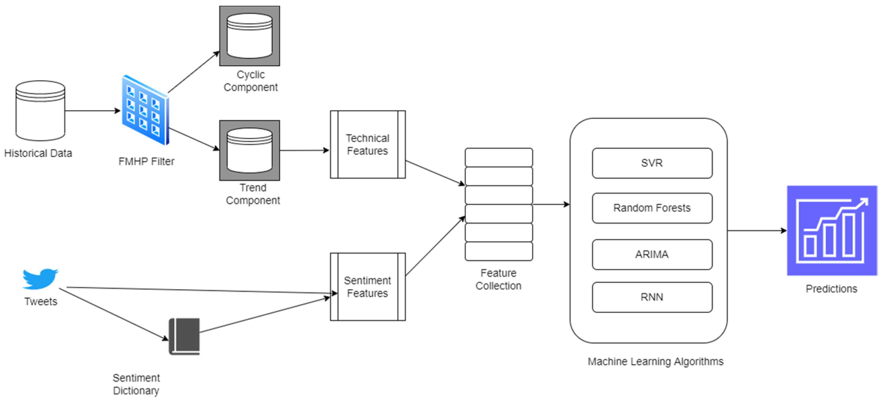
We propose a novel hybrid method comprising a fully modified Hodrick–Prescott (FMHP) filter [36], novel features proposed by Chen et al. [14], sentiment features, and a machine learning algorithm. The FMHP helps to remove noise and smooth the financial dataset. Novel features consist of stock price-features and sentiment features based on Twitter data. The machine learning algorithms used in the study include the Support Vector Regression algorithm, random forests, recurrent neural networks, and ARIMA. Figure 1 shows details of the proposed model. Our proposed model uses a historical stock dataset and a Twitter dataset. The historical stock dataset contains daily stock data of Apple Inc. (AAPL) over one year. The attributes include daily opening, close, highest, lowest, and average stock prices, and the total volume of stocks sold. The Twitter data comprise daily tweets about the same company over the same period. The historical stock data are passed through the FMHP filter to segregate cyclic and trend components. After removing the cyclic component from the stock price data, we input the trend component into the training model. The Twitter data are also preprocessed and fed into the training model along with the sentiment scores from the sentiment dictionary. The model learns from the provided data to make accurate predictions for the stock closing-price.

3.1. Datasets Used in the Model

We used two datasets for predicting stock closing-prices: historical stock-price data and Twitter data. The details of the dataset follow.

3.1.1. Historical Stock-Price Data

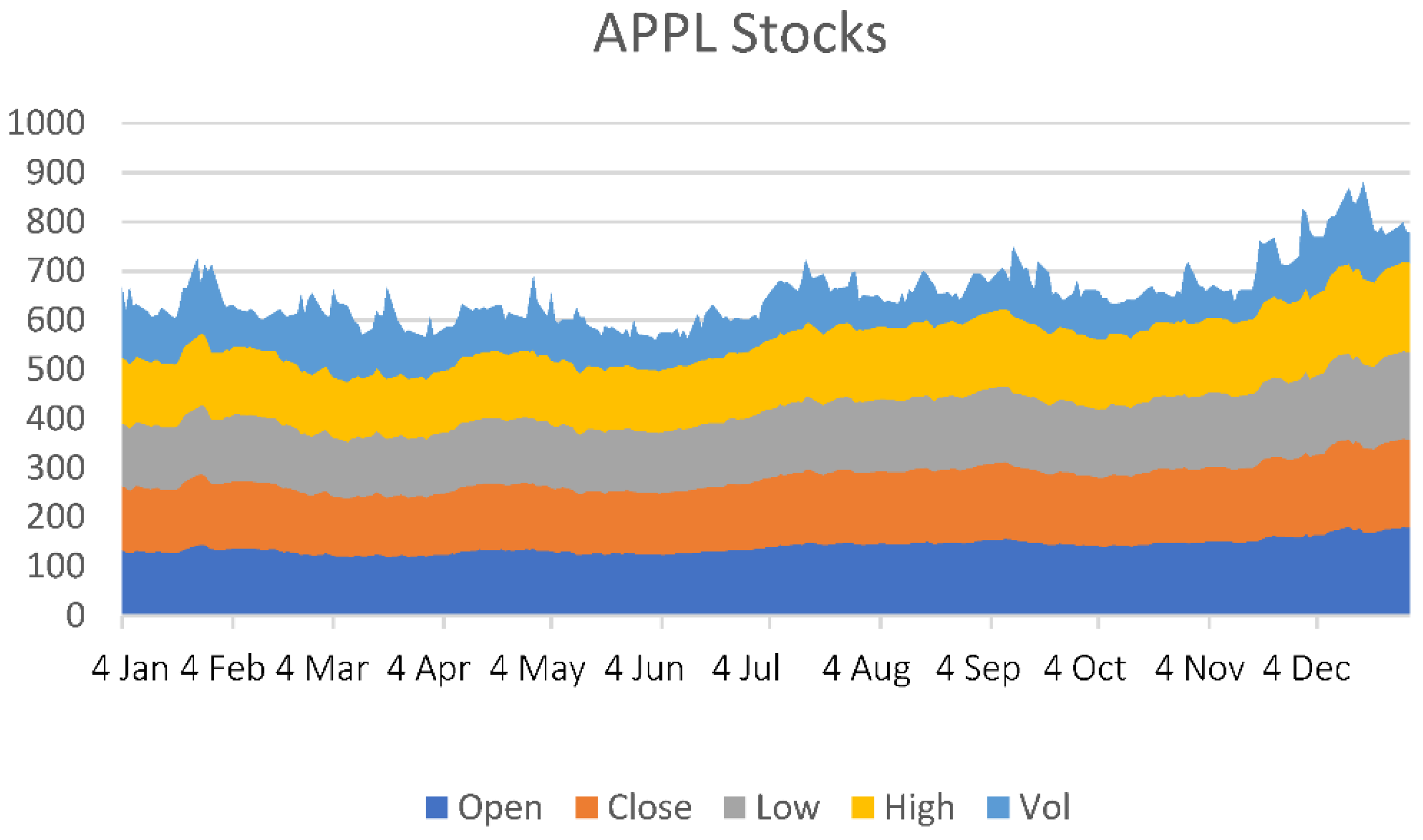
The historical data were obtained from the Yahoo Finance Stock Index. Yahoo Finance is part of the Yahoo network that provides financial news and international market data, including various stock quotes, released media, financial reports, commentaries, and other original content. Our data contain six attributes: date; closing price; open price; high price; low price; and volume for Apple Inc. Pvt. Limited (AAPL) from 4 January 2021 to 30 December 2021. Figure 2 shows a visual representation of the data. We aim to forecast the future closing price of AAPL for a given day. The closing price is the most accurate estimate of a security until trading commences over the next trading day, as it is used to measure market sentiment for the trading day.

3.1.2. Twitter Dataset

Social media has become an essential platform for analyzing public opinion and sentiments about any situation or event. Twitter is the most popular service for sentiment analysis because of its large number of users and public comments. Forecasting stock movement through social media has also recently gained traction. Sentiment analysis through tweets may help gather public opinion and determine stakeholders’ cumulative mood. Market activity correlates with public sentiments and opinions expressed by shareholders and experts in their tweets. We used tweets from Twitter for AAPL from 1 January 2021 to 30 December 2021, for sentiment analysis. The following section provides further details on tweet processing and novel sentiment features.

3.2. Data Preprocessing

Data preprocessing is an essential step for every machine learning model. We filtered the raw data for technical features to remove the noise and extract the financial trend component. For sentiment analysis, tweets were preprocessed using natural language processing techniques. Finally, we used a sentiment dictionary to support the sentiment analysis. The following sections provide details about these preprocessing steps.

3.2.1. Filtering Historical Data Using FMHP Filter

Hanif et al. proposed the endogenous lambda method to develop a fully modified Hodrick–Prescott (FMHP) filter [36]. The proposed technique resolves the end point bias issue of the Hodrick–Prescott filter by employing modifications in the weighting scheme and endogenous smoothing parameter. The FMHP first estimates λ endogenously and then estimates g_t (growth component) by using the leave-out approach of McDermott, using λ = 1 as the starting value. The working of the FMHP filter is explained in [36]. The main changes applied in Hodrick–Prescott filer are:

• Use of linear or nonlinear increase of penalization, which minimizes cumulative loss at terminal points;
• g_t denotes the growth component of y_t where y_t = g_t + c_t, c_t is the cyclic component of y_t;
• Fixed the value of k = 20;
• Endogenous weights (for end observations) i.e., endogenous α.

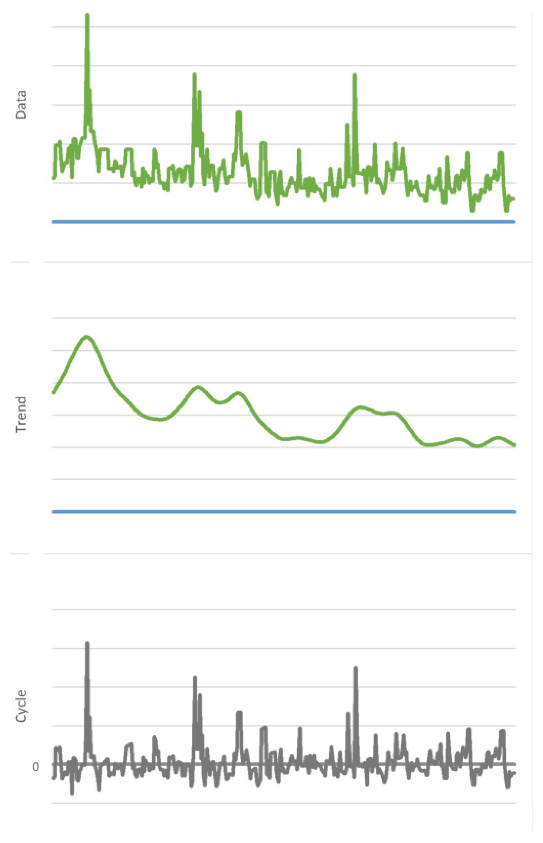
Figure 3 shows the trend and cyclical component extraction after applying a fully modified HP Filter on time series data. It can be observed that the trend component is more suitable for prediction because of its smoothness. However, the cycle component has abrupt peaks and valleys, suggesting it should be filtered for making accurate predictions.

3.2.2. Prediction Features

Chen et al. proposed a set of novel features for predicting stock closing-prices [14]. In addition to their proposed features, we present another set of features for making more accurate predictions.

Table 1. Technical features with formulae.

Sr	Technical Feature	Description
1	Ot	The opening price of the stock on day t
2	Ct	The closing price on which the stock is traded on day t
3	Ht	The highest price of the stock during day t
4	Lt	The lowest price of the stock during day t
5	Vt	The total volume of stock shares traded during day t
6	$V_t-V_{t-1}$	Volume change [14]
7	$\frac{V_t-V_{t-1}}{V_{t-1}}$	Volume limit [14]
8	$\frac{H_t-L_{t-1}}{C_{t-1}}$	Amplitude [14]
9	$\frac{C_t-O_{t-1}}{C_{t-1}}$	Difference [14]
10	$R_{t,f}=$$\mathrm{LN} (\frac{ C_{t,f}}{ C_{t-1, f}})\times 100\%$	Return of firm f at time t
11	$\mathrm{ROP}=O_t$$-O_{t-1}$	(Return open price) open-to-open
12	$\mathrm{RCP}=C_t$$-C_{t-1}$	(Return close price), close-to-close
13	$\mathrm{DROP}=\frac{ C_t-C_{t-1}}{C_{t-1}}$	Change in return open price
14	$\mathrm{DRCP}=\frac{{\mathrm{C}}_{\mathrm{t}}-{ \mathrm{C}}_{\mathrm{t}-1}}{{\mathrm{C}}_{\mathrm{t}-1}}$	Change in return close price
15	$\mathrm{VPT}={ \mathrm{VPT}}_{t-1}+ V \times \frac{\left(C_t-C_{t-1}\right)}{ C_{t-1}}$	VPT (volume per total) is measured when the volume is multiplied by the change price and is calculated as the running price total from the prior period

shows the features proposed by Chen et al. and the proposed features, along with a brief description and formula for calculating each feature. The features from 1–5 are the basic features of the dataset. Features 6–9 are proposed by Chen et al. [14]. The rest of the features are derived from basic features and are proposed in this study.

3.2.3. Twitter Dataset

We used Twitter data for AAPL from 4 January 2021 to 30 December 2021. After collection, the Twitter data are first preprocessed. First, we arrange per-day tweets. The entire text is converted into lowercase. After that, we remove numbers, punctuation, stop words, and URLs.

3.2.4. Domain-Specific Dictionary to Calculate Sentiment Features

Studies have reported that social websites and related information can help improve prediction effectiveness [41]. To this end, studies have included a sentiment dictionary to use sentiment scores from a large corpus. A sentiment dictionary contains pairs of selected words and their sentiment values. Predicting stock market fluctuation also involves analyzing public sentiment on social media in addition to the patterns of the stock market price. We calculate the frequency of each keyword for all tweets on a given day. The mean sentiment for each keyword is calculated by using a domain-specific dictionary. We use the arithmetic mean to estimate cumulative sentiment for a given day by using sentiment scores for all keywords. We used the sentiment dictionary developed by Hamilton et al. [42].

3.3. Prediction Models

We used four machine learning algorithms to predict stock closing-prices, including support vector regression, random forests, ARIMA, and recurrent neural networks. The details of these models are presented in the following sections.

3.3.1. Support Vector Regression

Vapnik developed the theory of support vector regression (SVR) when he used support vector machines to solve a regression problem [43]. The fundamental idea behind the SVR is to transform a nonlinear dataset into a high-dimensional feature space and apply linear regression to this feature space. Consider a dataset X where x_i ∈ X = R_n is an input vector, y_i ∈ Y = R of the matching output value, the SVR function is:

$$f\left(x\right)=w·\phi \left(x\right)+b$$

(3)

where φ(x) is a nonlinear mapping function; w is the weight vector; and b is a bias value. This function can be evaluated by minimizing the risk function:

$$R\left(w\right)=\frac{1}{2} \Vert w{\Vert }^2+C{\sum }_{i=1}^l{L}_e\left(y_i,f\left(x_i\right)\right)$$

(4)

where $\frac{1}{2}\Vert w{\Vert }^2$ is a flatness function; and C is the penalty parameter that describes the trade-off between training error and generalized performance. Let L_e(y_i, f(x_i)) be an insensitive loss function described as:

$$L_e\left(y_i,f\left(x_i\right)\right)=\{\begin{array}{c}\left|y_i-f\left(x_i\right)\right|-\epsilon , if \left|y_i-f\left(x_i\right)\right|\ge \epsilon \\ 0,if \left|y_i-f\left(x_i\right)\right|<\epsilon \end{array}$$

(5)

In the above, $\left|y_i-f\left(x_i\right)\right|$ is defined as the predicting value of an error, and ε is defined as a loss function when error for estimation is taken into account by using two positive slack variables ζ and ζ*, which represent the difference between original values corresponding to boundary values.

3.3.2. Recurrent Neural Networks

Recurrent neural networks (RNN) can handle the sequence of dependencies and are often used for time series prediction [1,44]. RNNs are called recurrent as they accomplish the same task for every element in the sequence, and their current output depends on previous calculations. In our work, RNN used the input value of the t-th day x_t = (x_t,1, x_t,2, …, x_t,m) where m-vector indicates the features described in prior subsections. The algorithm iterates over the following equation:

h_t = tanh (Ux_t + Wh_t−1 + b)

(6)

o_t = tanh (Vh_t + c)

(7)

where h_t denotes the hidden state calculated based on previous hidden states h_t−1 and input x_t for the current time step; o_t is the predicted output, which is considered a stock price indicator for subsequent trading. RNN trained three parameters, U, V, and W, where U indicates input-to-hidden, V hidden-to-hidden, and W hidden-to-output states.

RNN trained itself based on long arbitrary information in the sequence. Due to the vanishing gradient issue, RNNs cannot learn long-term dependencies. To tackle this issue Chung et al. [45] proposed Gated Recurrent Units (GRU, where r_t and z_t are known as reset gates which utilize the combination of new input x_t with earlier memory h_t−1 for computing s_t). The s_t determines a “candidate” hidden state. Update gate z_t helps h_t calculate the required space for the previous memory. The following equations are used for the calculation of GRU:

z_t = σ (x_tU_z + h_t−1W_z + b_z)

(8)

r_t = σ (x_tU_r + h_t−1W_r + b_r

(9)

s_t = tanh (x_tU_s + (h_t−1 ⊙ r_t) W_s + b_s)

(10)

h_t = (1 − z_t) ⊙ s_t + z_t ⊙ h_t−1

(11)

where σ(x) is the hard-sigmoid function and ⊙ represents the Hadamard product. We applied a two-hidden-layer GRU component and captured the higher level of feature interactions between different time phases. Units in the second hidden layer are intended to be similar to the first hidden layer.

To train the RNN, we input the feature vectors of a specified period from t₀ to t_n, as training data and observe values as a target value, i.e., {x₁, x₂, …, x_n} and {y₁, y₂, …, y_n} correspondingly. Here we calculate the dependent variable, which is y_i = C_i/C₀ − 1, i = 1, …, n, wherever C₀, …, C_n are taken as the closing price. Historical data of previous s days are used to predict the price of the n trading day—the starting parameters of the GRU unit set by using predefined seed as a guarantee repetitive of RNN models. GRU uses a backpropagation approach to train the parameters by minimizing the difference between the o_t (output) and observed values y_t. For the performance evaluation of our proposed model, the total time interval is divided into two steps—data from t₀~t_m−1 are used for training (GRU parameters) and predict t_m~t_n as dependent data. In the second step, the GRU parameters are updated after new predictions are calculated, i.e., o_t+1, where y_t is the input into the GRU module for training. It simulates a real-world situation for new stock prices because the new price can be obtained daily and used as input for training.

Another very powerful technique based on RNN is LSTM. It can deal with sequential data and is highly suitable for training and testing stock market value prediction. This technique is capable of learning long-term dependencies among data. The underlying working principle of LSTM is the same as GRU, except that this technique has some additional gates. The addition of memory cells can help combat vanishing gradients. It consists of four units: an input gate; an output gate; a forget gate; and a self-recurrent neuron. These gates control the interactions between neighboring memory cells and the memory cell itself. The input gate controls the influence of the input on the memory cell, while the output gate controls the amount of memory to retain. Lastly, the forget gate controls how much history to remember or forget.

3.3.3. ARIMA

Autoregressive Integrated Moving Averages (ARIMA) is a statistical model used to predict and analyze time series data [46]. ARIMA establishes the relation between some delayed observations and current observations by applying the moving average. ARIMA has three standard representations; lag order p represents the number of lag observations included in the model, degree of differencing d represents the number of times the differences are calculated for raw observations, and q represents the size of the moving average window. A model is created by configuring the above-specified terms for forecasting a result variable. A value of zero can be used for the parameter with the element that the model will not use.

3.3.4. Random Forests

A random forest (RF) is an ensemble of classifiers that makes predictions by combining the results from many individual decision trees [47]. It is similar to the bagging method but offers an improved way of bootstrapping. A random forest generates a set of classification and regression tree (CART)-like classifiers. For regression problems, an average of all predictions is calculated. Classification problems use a majority vote scheme. We used the boosting method for its simplicity. Technically, feature sampling is used to generate a subset of data. The number of features used for splitting is an adjustable user-defined parameter. It is worth noting that limiting the number of split features can reduce the algorithm’s computational complexity. In addition, it can help process high-dimensional data efficiently and define relatively deeper trees. The final results are then obtained by averaging the individual results obtained from each subtree.

4. Experimental Results

This section describes the experimental setup and the quantitative results obtained from the proposed model. As explained above, the experiments are executed using two datasets, time series, and Twitter datasets for AAPL Inc. (Los Altos, CA, USA) during the same period. The details of the experimental setup and results follow.

4.1. Experimental Setup

This study aimed to perform a day-ahead stock closing–price prediction. We used two weeks (14 days) of historical samples as input to train the model and then predict the stock closing-price of the next day. The recursive rolling strategy was employed for processing both training and testing data. The time series data were transformed into M × N matrix using the phase space reconstruction method, where M represents the number of days set to 14 and N is the number of samples. Before running the experiments, we divided the data into training (80%) and testing (20%) datasets. We used cross-validation to identify the optimal parameters for the classifiers. We applied a grid search algorithm to determine the optimal parameters for each classifier.

We selected SVR with radial basis function (RBF) for its excellent performance. The optimal values for two essential parameters required for RBF, cost (C) and gamma (γ), were selected as 275 and 0.1, respectively. The performance of SVR depends on the choice of kernel. We used the RBF kernel, which is a popular kernel in SVMs.

Table 2. Kernel parameter settings.

Regression Model	C	G	D
SVR	250	0.01	3
SVR + HP	275	0.1	3
SVR + FMHP	285	0.1	3
SVR + FMHP + Novel Features	285	0.1	3

gives the selected kernel parameters for various regression models. Here G represents the kernel parameter, D is the degree, and C is the penalty.

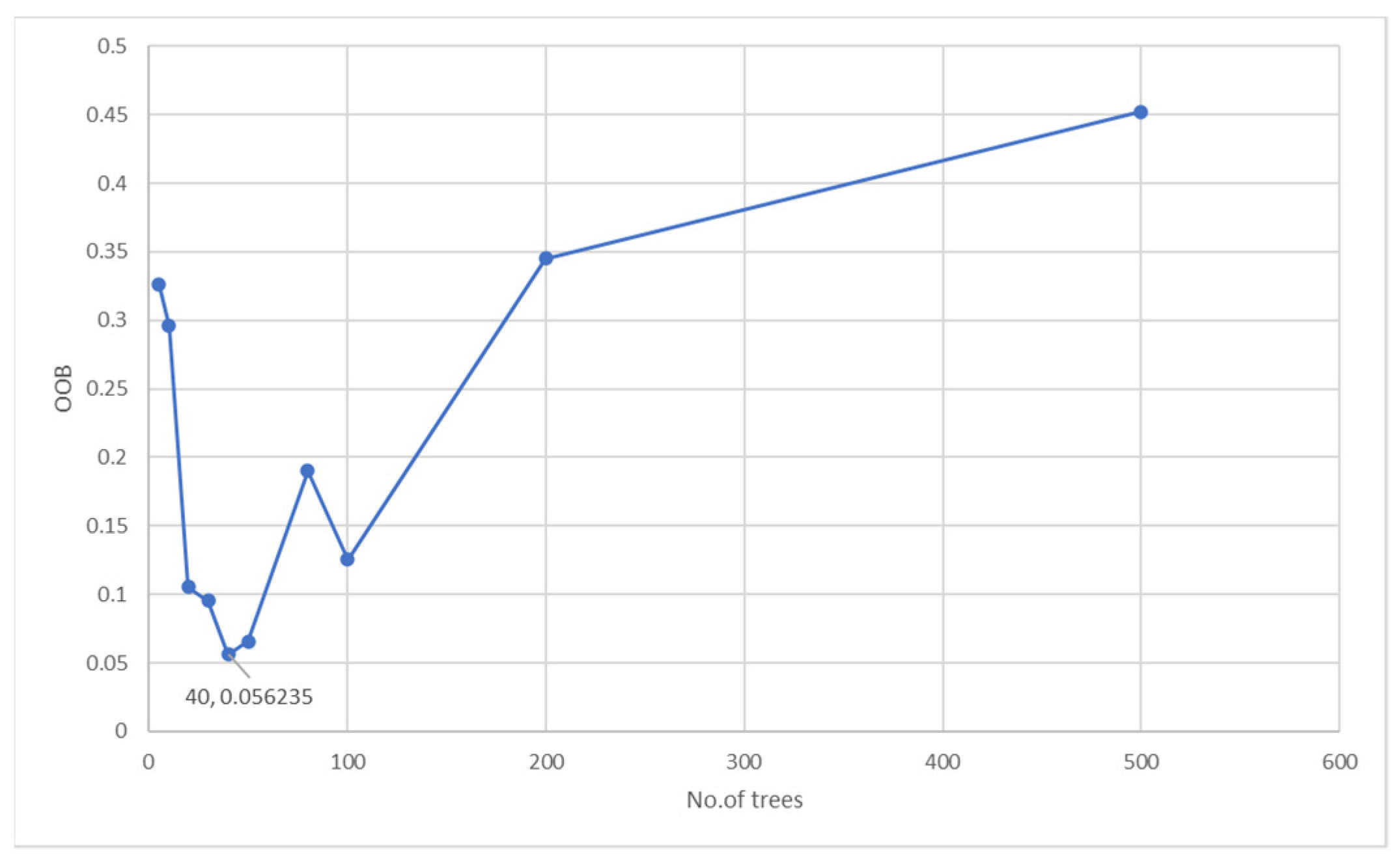
For random forests (RF), we fine-tuned two parameters, the number of decision trees (n_t), and the maximum number of features considered at each split (n_f). We empirically set the values for both parameters, i.e., n_t = 40 and n_f = 4. As RF is less sensitive to n_f, we set it to a constant value. We performed convergence tests for the RF on the training set to find the optimal values for its parameters. It is worth mentioning that, initially, the RF accuracy increased as we increased the number of trees. However, after the number of the trees reached 40, we did not see any further improvement in out-of-bag error (OOB). Therefore, we selected this value as the optimal value for training. Figure 4 summarizes the OOB for ten iterations for a time window of 30 days on the training data. The choice of splitting criteria was defined using the Gini impurity.

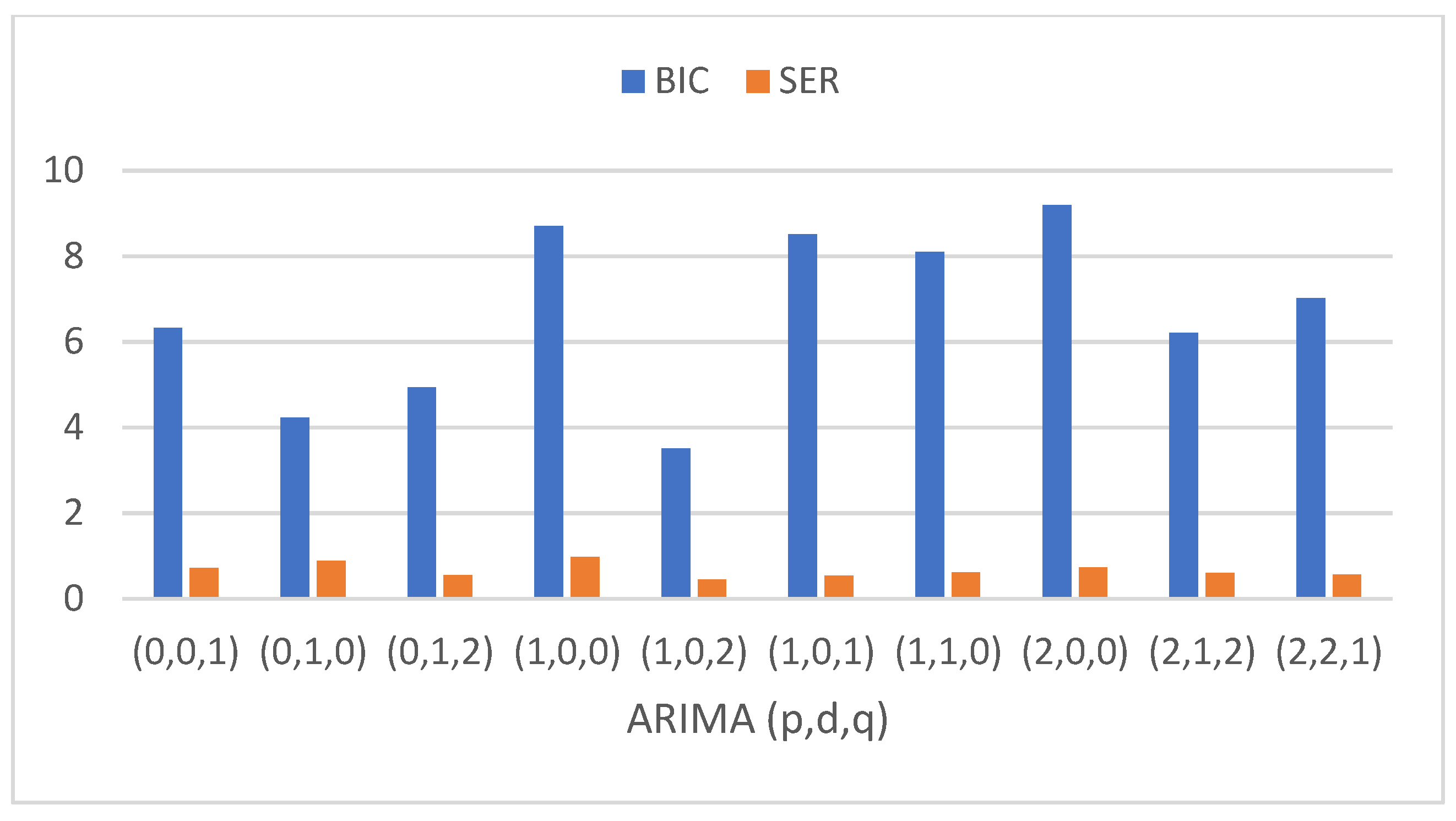
There are three critical parameters for the ARIMA model, the number of autoregressive terms (p), the number of nonseasonal differences needed for stationarity (d), and the number of lagged forecast errors (q). We set the values of p, d, and q to 1, 0, and 2, respectively. Figure 5 summarizes various combinations of the parameters and their corresponding standard error of regression (SER). It shows that the best relative results were obtained for the parameter setting of (p, d, q) = (l, 0, 2). The lowest value for the Bayesian information criterion (BIC) obtained was 3.5042 and a relatively smaller SER of 0.443804.

We used two popular variations of the RNN, namely LSTM and GRU. The overall architecture and parameters for both variations were the same. We used four layers with 50 units in each layer with a hyperbolic tangent function as its activation. The learning rate was set to 0.01, and the Adam optimizer was used. Since the data were reduced in size, therefore, no dropout was considered. We used the hyperbolic tangent function because its derivative is late in approaching 0, which helps in learning longer sequences. We adopted different types of seeds for the initialization of our model. The average was measured based on 100 rounds using 0 to 99 seeds of experiments.

4.2. SVR Results

The SVR was trained on the training dataset for a time window of 30 days and then we tested the prediction accuracy on our test dataset. The following settings were used for training the model:

• The basic SVR model;
• SVR and sentiment features;
• SVR with HP filter;
• SVR with HP and sentiment features (denoted as Sent);
• SVR with FMHP filter;
• SVR with FMHP filter and sentiment features.

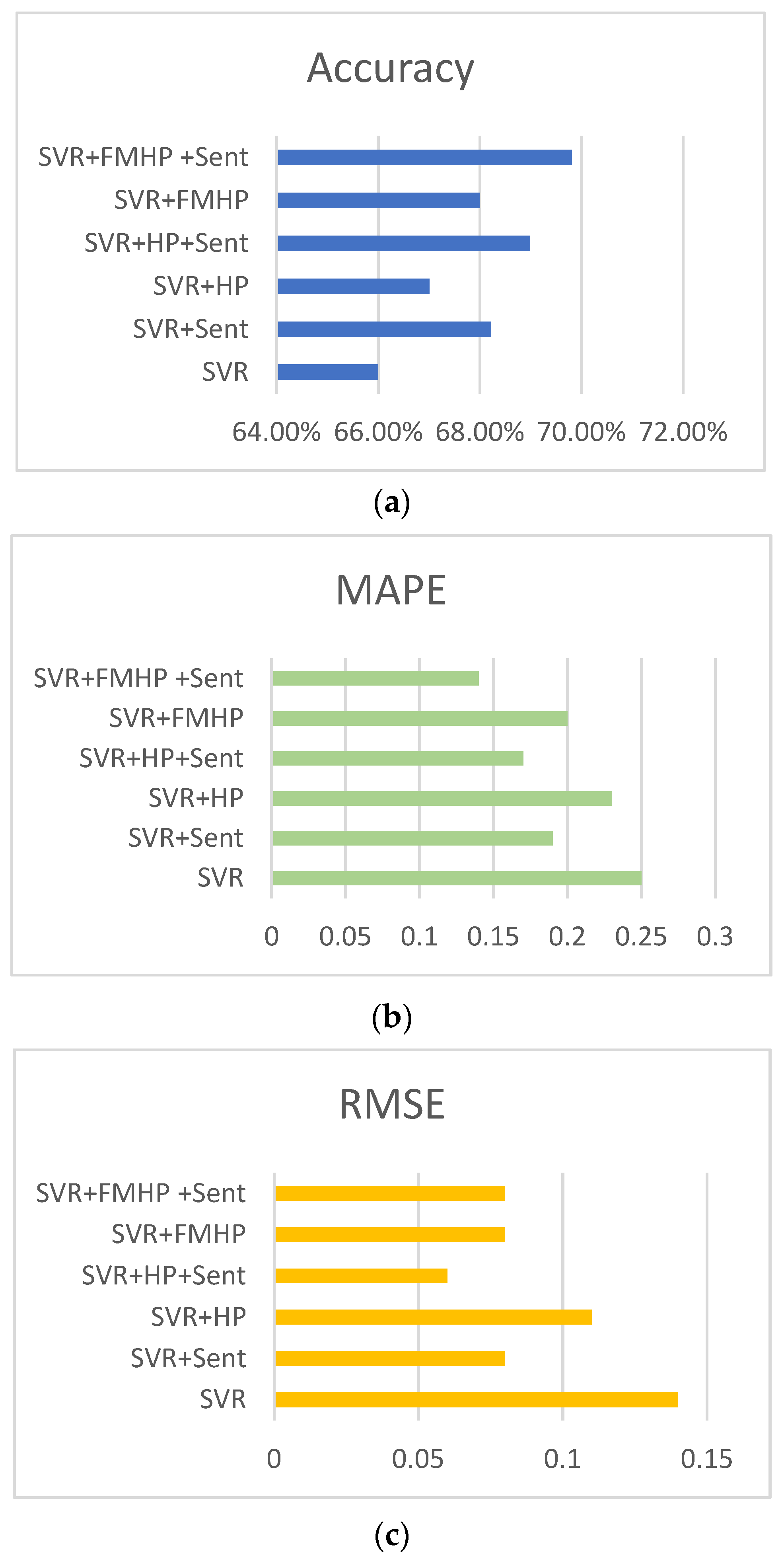
The results obtained for predicting the closing price of AAPL stock for these training settings are summarized in Figure 6. The prediction accuracy of the base SVR model was 66% which improved to 68.22% with sentiment features. Using sentiment features, the MAPE and RMSE improved by 24% and 42.86%, respectively. The HP filter with SVR achieved 67.01% accuracy, which increased to 68.99% when sentiment features were incorporated into the model. An improvement of 21.05% and 37.50% was observed in MAPE and RMSE, respectively. Finally, the prediction accuracy, MAPE, and RMSE were 68%, 0.2, and 0.08 with the FMHP filter. The corresponding measures improved to 69.81%, 0.14, and 0.08 when the model was augmented with sentiment features. We can conclude that the most sophisticated model improved accuracy by 5.46%, MAPE by 44%, and RMSE by 42.86% compared to the basic SVR model.

4.3. Random Forests Results

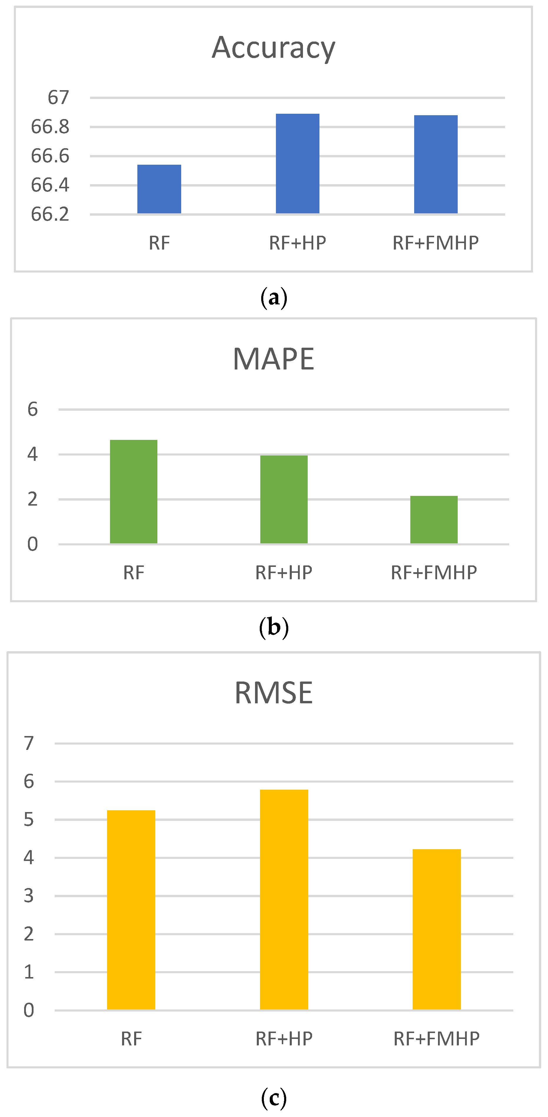
The results obtained using RF are summarized in Figure 7. The highest accuracy (66.89%) was achieved for the combination of RF with the HP filter, although the base RF model (66.54%) and the RF with FMHP (66.88%) also gave a comparable prediction accuracy. However, the overall results indicate that FMHP outperformed the HP filter and the base SVR models. Using HP improved MAPE and RMSE by 53.66% and 19.47%, respectively.

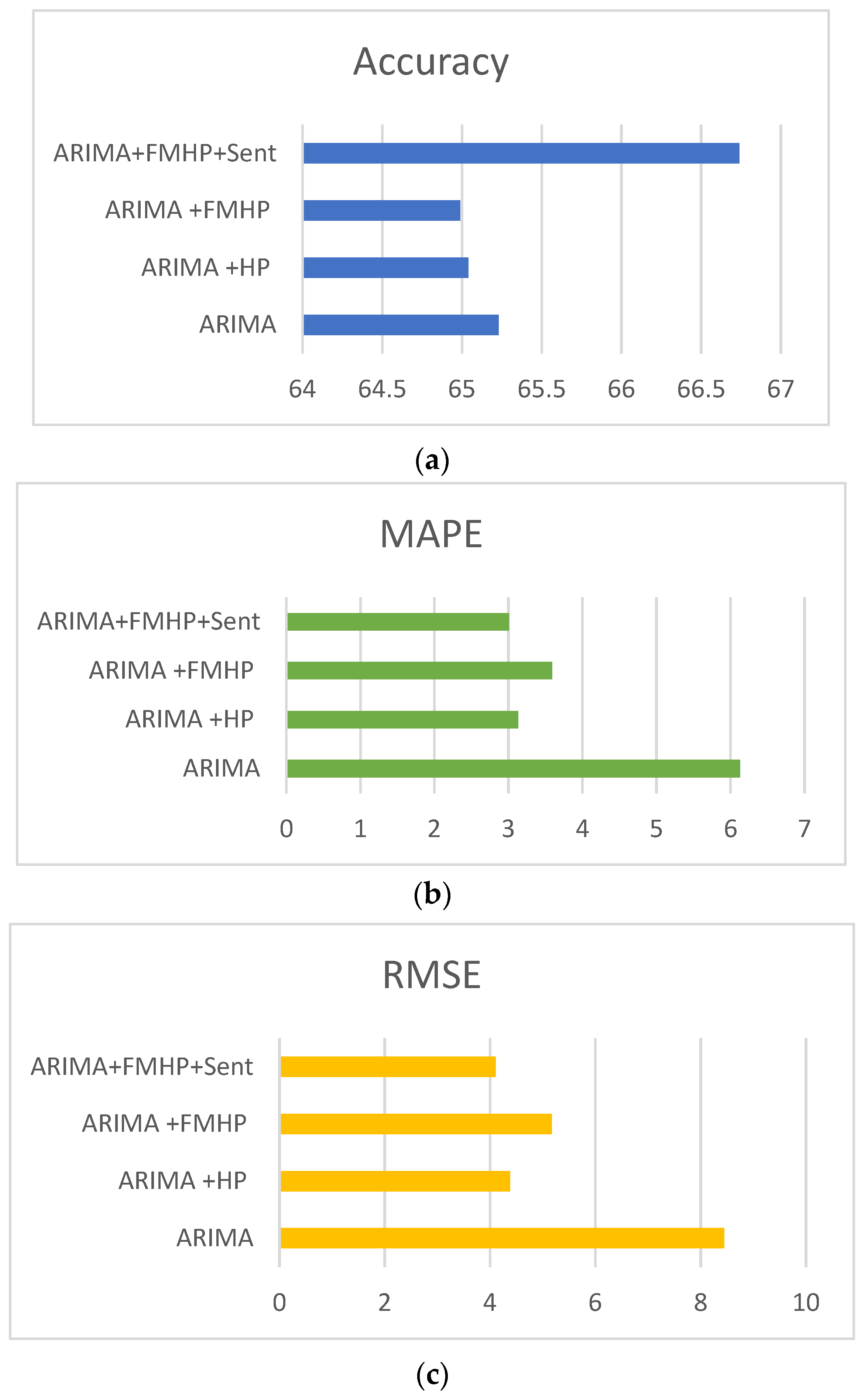
4.4. ARIMA Results

Figure 8 summarizes the results obtained for the ARIMA model for the prediction of the AAPL closing price. The best results obtained for ARIMA+HP+Sent with MAPE and RMSE on the test were 3.01 and 4.11, respectively. The prediction accuracy of the models was 66.74%. Although the performance gain for accuracy is not significant (1.51%), the MAPE and RMSE were improved significantly (3.12 and 4.34, respectively) using the FMHP filter with the base ARMIA model.

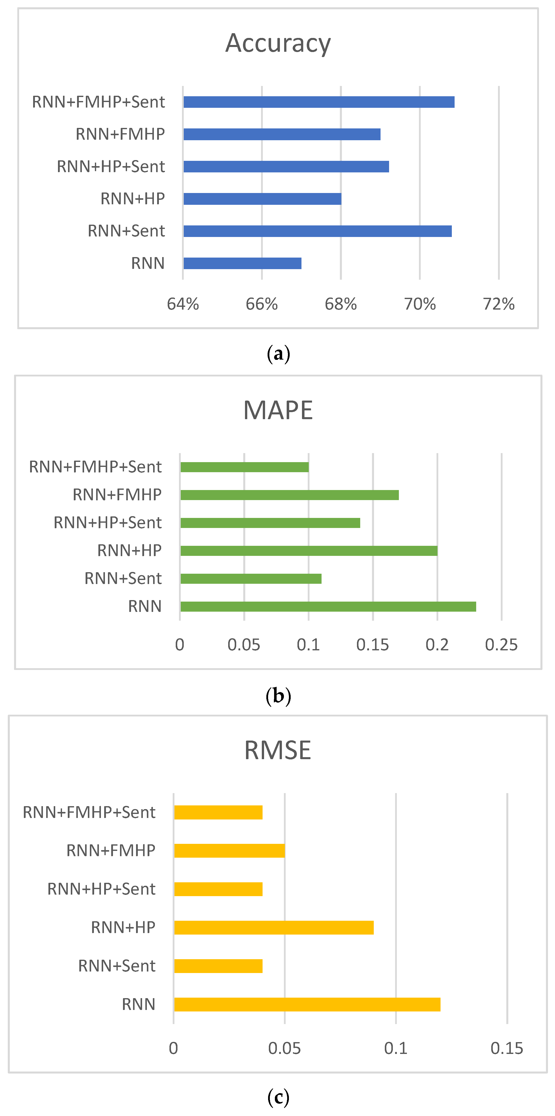
4.5. Recurrent Neural Network Results

We used a two-layer RNN model [48] combination with GRU and compared the model’s performance with and without noise filters. The results are shown in Figure 9. The prediction accuracy of the base RNN model was 67%, which improved to 70.81% when sentiment features were also included in the model. The MAPE improved from 0.23 to 0.11 for the respective models. Similarly, the respective models improved from 0.12 to 0.04 for the RMSE measure. The prediction accuracy of RNN+HP was 69.01% which improved to 69.22% when sentiment features were also used. The corresponding figures for MAPE improved from 0.2 to 0.14 and from 0.09 to 0.04 for RMSE. Finally, RNN with FMHP performed 69% accurate predictions, which became 70.88% when sentiment features were incorporated into the model. Similarly, MAPE went from 0.17 to 0.1 and RMSE from 0.05 to 0.04. It can be concluded that using FMHP and sentiment features improved the accuracy of the base RNN model by 3.88%, MAPE by 56.52%, and RMSE by 66.67%.

After comparing the results of all machine learning algorithms used in the study, we conclude that RNN with FMHP filter and sentiment features achieved the best performance for all evaluation measures.

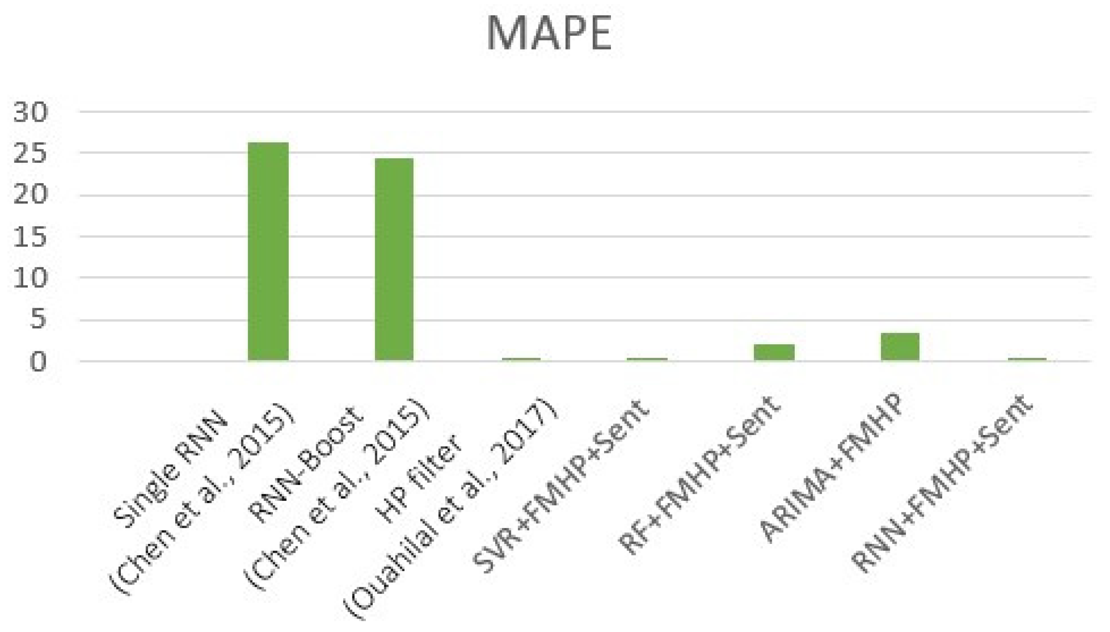
4.6. Comparison of the Proposed Model with Other Studies

We compared our results against two related models because our proposed model is an extension of two models. First, we have extended the features proposed by Chen et al. [14]. Secondly, Ouahilal et al. [15] used the HP filter for stock closing-price prediction, while we used the fully modified HP filter. Ouahilal et al. have given only the error rate in the results. Figure 10 provides a comparison of the error rates of these models. The best MAPE achieved by Ouahilal et al. was 0.07. Our best model, RNN+FMHP+Sent, achieved slightly higher MAPE than their model (0.1). However, our results were significantly better than MAPE values of 26.21 and 24.31 performed by two models proposed by Chen et al.

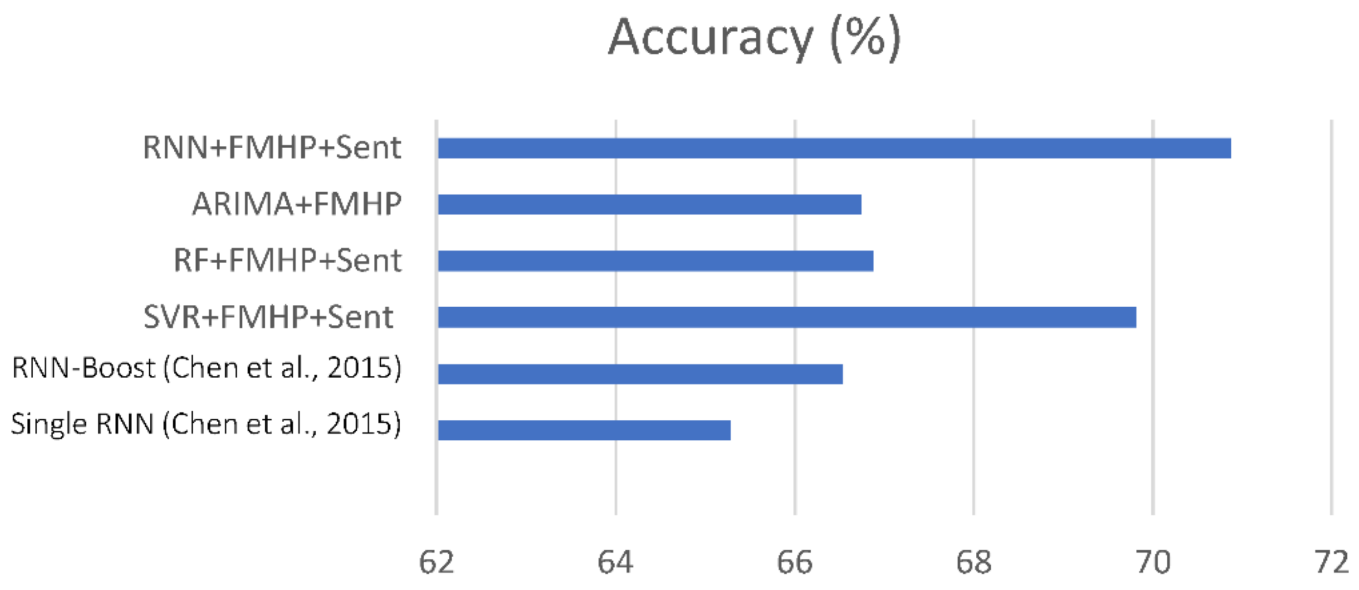
Our model also outperformed the models proposed by Chen et al. for other measures. Figure 11 shows that our best models achieved a 70.88% prediction accuracy which is significantly better than the 65.28% and 66.54% performed by the models of Chen et al.

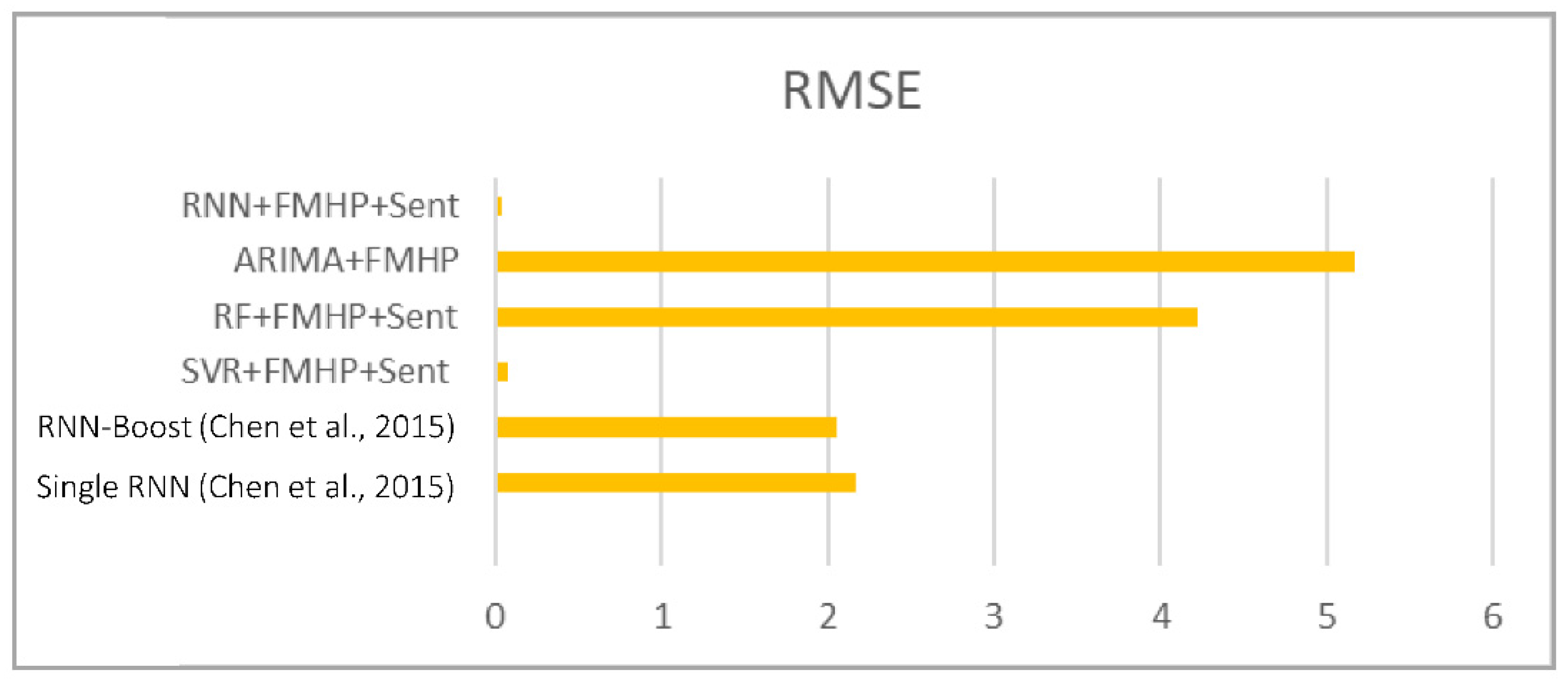
Our best model also achieved a significantly lower RMSE (0.04) compared to the best RMSE score of 2.05 achieved by Chen et al. Figure 12 shows a visual comparison of our models with their models.

5. Discussion

The HP filter minimizes fluctuations in time series against parameters that approach linear trends. FMHP is an extended HP filter that produces trend and cyclical components, lowers the endpoint base (EPB), and performs comparatively better than the HP filter. The trend component produced by the BK filter or CF filter slightly changes the time series curve. In our experiments, we found that the trend component produced by the HP filter preserved the financial series curve hence improving endpoint bias.

We conducted several experiments using different approaches to compute the performance of predicting stock price and our proposed model. Both technical and content features were combined to improve prediction accuracy. The performance of machine learning methods was investigated on original data, as well as applying some noise reduction techniques, including HP and FMHP filters. We found that HP and FMHP are effective for noise reduction and work efficiently to improve the model’s prediction accuracy. In addition, the technical and content features complement each other and help reduce MAPE and RMSE error rates.

6. Conclusions

This study aimed to investigate the best combination of machine learning and noise reduction techniques for predicting the closing stock price. Two types of features were obtained, technical features were derived from the historical stock data, while content features were obtained from official accounts of Twitter. Technical and content features were combined to improve prediction accuracy. We used five machine learning approaches, three traditional, and two deep learning-based approaches. Two approaches for time series data denoising were evaluated: FMHP and HP. We performed several experiments in combination with machine learning approaches for prediction of AAPL stock value prediction using 14 days of historical data. The proposed model using our hybrid technique and combination of ML and DL models, the FMHP noise filter, and the new technical and content features, is a powerful predictive tool for analyzing stock market price prediction, content, and financial time series.

The stock market price depends not only on time series data but also on macroeconomic factors, and other external factors, such as the news, significantly impact the stock market price. These types of limitations lead to some issues which need to be solved for future research. In the future, we will extend our work to improve the prediction accuracy for longer historical data and reduce the processing time for deep learning methods. We also intend to validate the proposed novel features and the FMHP filter with a more diverse dataset. Moreover, the hyper-parameter tuning is also complex. Therefore, an automatic hyper-parameter selection approach will be adopted to obtain optimal parameters.