Article

Improved YOLOv3 Model for Workpiece Stud Leakage Detection

School of Mechanical and Automotive Engineering, Guangxi University of Science and Technology, Liuzhou 545006, China
*
Authors to whom correspondence should be addressed.
Electronics 2022, 11(21), 3430; https://doi.org/10.3390/electronics11213430
Submission received: 17 September 2022 / Revised: 19 October 2022 / Accepted: 20 October 2022 / Published: 23 October 2022

Abstract

:
In this study, a deep convolutional neural network based on an improved You only look once version 3 (YOLOv3) is proposed to improve the accuracy and real-time detection of small targets in complex backgrounds when detecting leaky weld studs on an automotive workpiece. To predict stud locations, the prediction layer of the model increases from three layers to four layers. An image pyramid structure obtains stud feature maps at different scales, and shallow feature fusion at multiple scales obtains stud contour details. Focal loss is added to the loss function to solve the imbalanced sample problem. The reduced weight of simple background classes allows the algorithm to focus on foreground classes, reducing the number of missed weld studs. Moreover, K-medians algorithm replaces the original K-means clustering to improve model robustness. Finally, an image dataset of car body workpiece studs is built for model training and testing. The results reveal that the average detection accuracy of the improved YOLOv3 model is 80.42%, which is higher than the results of Faster R-CNN, single-shot multi-box detector (SSD), and YOLOv3. The detection time per image is just 0.32 s (62.8% and 23.8% faster than SSD and Faster R-CNN, respectively), fulfilling the requirement for stud leakage detection in real-world working environments.

1. Introduction

With the rapid development of science and technology, intelligent industrial production lines are gaining popularity, and the control of production quality by enterprises is becoming increasingly stringent. The ability to identify studs accurately and at a high speed directly determines the intelligence and efficiency of the production line. This is a key issue in the quality control of automotive companies. The traditional method of manually identifying studs is unsuitable for the intelligent development of automotive production lines for many reasons, such as its slow detection speed, low efficiency, high false detection rate, tendency to cause fatigue, and the partly luminous and heat-generating workpieces, which are harmful to the human eye [1].
In response to the problems with manual inspection methods, experts and researchers have conducted extensive research on contactless inspection methods.
Traditional processing methods are primarily based on lasers, ultrasonic sensors, and manual feature extraction. Auerswald et al. [2] used laser lines to detect fractures and defects in large gear workpieces. Li et al. [3] proposed an industrial inspection method based on multilaser scanner point clouds with high detection accuracy; however, these sensors are expensive. Guo et al. [4] used ultrasonic technology to detect defects on the workpiece surface, which achieved good results in terms of cost reduction but failed to achieve better optimization in terms of reliability and visualization. With the continuous development of computer vision techniques, the extraction of manually designed features from workpiece images to achieve the rapid recognition of defects has become a popular topic in industrial inspection. Lee et al. [5] developed a histogram-based workpiece recognition method and used the difference, mean, and standard deviation to analyze workpiece images for recognition. Kumar et al. [6] proposed a method for workpiece welding recognition based on the gray-level co-occurrence matrix, which is suitable for the texture recognition of workpieces. However, both methods require certain assumptions, e.g., a separable workpiece detection region. Therefore, they cannot detect the scene in the entire field of view, and the methods are very sensitive to hyperparameter settings. Zhang et al. [7] proposed a detection method for aluminum alloy wheel artifacts that incorporated adaptive threshold segmentation and morphology. However, the improper selection of smoothing operators and thresholds can cause the method to fail to extract image features. Shi et al. [8] proposed an improved Sobel detection algorithm for railway track surface artifact identification that uses filters to reduce image noise and remove artifact surface defect features. This method uses a filter to reduce image noise and extract features from the surface of the workpiece. However, it is not suitable for all random texture images and suffers from feature correlation. These methods are limited by the need to design explicit features based on the actual working conditions of the workpiece. Expert knowledge and manual design are essential, and the omission of key features, for example, can lead to poor detection results. As a result, these methods are more difficult to automate efficiently.
With the increase in hardware computing power, deep learning-based recognition methods are now used in various fields to automatically acquire target features and their valid information without requiring the manual design of the explicit features of the object to be detected. This advantage effectively avoids the problem of traditional recognition methods that require expert knowledge and manual configurations. In recent years, convolutional neural networks (CNNs) [9] have been extensively used in the field of workpiece stud image recognition and target detection [10,11]. Liu et al. [12] proposed an online stud measurement method based on photometric stereo measurements and deep learning theory. It uses a CNN to determine the key points of screws on automotive workpieces and can measure multiple studs with high accuracy. Current target detection algorithms in deep learning can be broadly classified into two main categories: those based on candidate regions and those based on regression [13]. Candidate region-based target detection algorithms are also known as two-stage approaches, i.e., the target detection problem is divided into two stages. Candidate regions are generated in the first stage. For example, Ren et al. [14] proposed the Faster R-CNN algorithm, which effectively speeds up the detection rate. Wang et al. [15] proposed an automatic tag welding robot based on a cascaded R-CNN target detection system that automatically identifies and picks up screws for welding.
Although the two-stage algorithm can achieve high accuracy in target detection [16], it still requires a selective search algorithm to generate candidate regions. Hence, the detection speed is inevitably limited by the need for repeated candidate region selection.
Regression-based detection techniques have emerged as solutions to above issue, requiring only one stage and performing regression directly on the projected target. Redmon et al. [17] proposed the YOLO (You Only Look Once) algorithm, which concentrates on classification, localization, and detection in a single network. The input image can directly obtain the bounding box and predicted value of the target in the image after only one network calculation. However, because of the crude design of the network, it cannot satisfy the accuracy requirements of real-time target detection. Small and multiple targets cannot be accurately localized and are easily missed. Redmon et al. proposed the YOLOv2 [
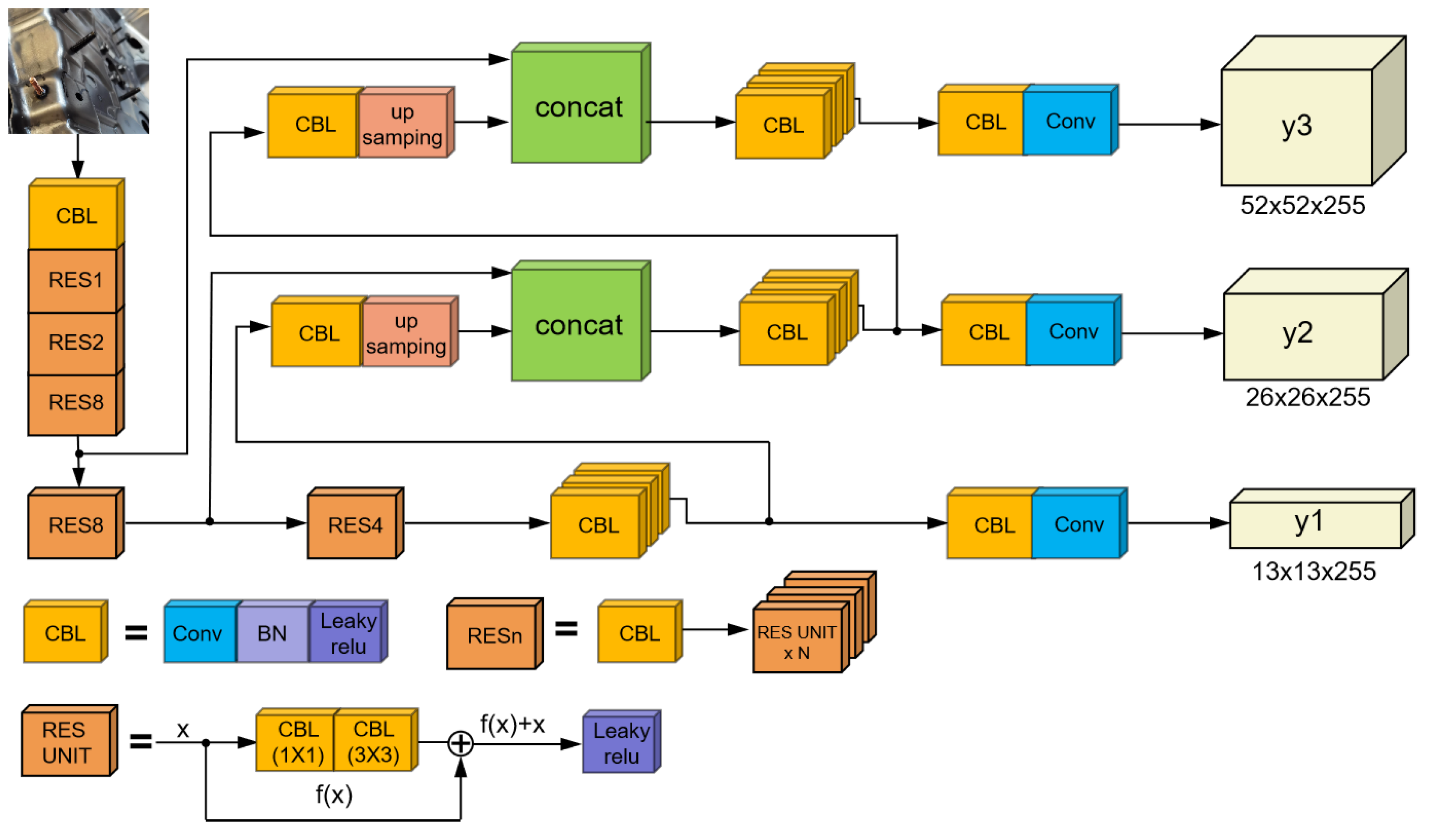
18] and YOLOv3 [19] models. YOLOv3 is an updated version of YOLOv1 and YOLOv2 that introduces the feature pyramid concept and adds a batch normalization (BN) layer to the boundary prediction. It predicts large, medium, and small targets at three scales by adding multiscale prediction and a basic backbone network [20,21,22]. However, when targeting small targets, the traditional YOLOv3 model fails to detect large or medium targets [23]. Missed weld stud detection on automobile workpieces is a classic example of the challenge of tiny target detection in a complex environment. Hence, this paper proposes a new deep learning algorithm to achieve automatic feature extraction and general detection model to solve the problem of the real-time detection and localization of studs on automobile workpieces. The improved YOLOv3 deep learning algorithm is based on the traditional YOLOv3 network model, and this study improves and optimizes it using an image pyramid structure and focal loss function. The following is a description of this study’s main contributions. Experiments show that these methods are effective.
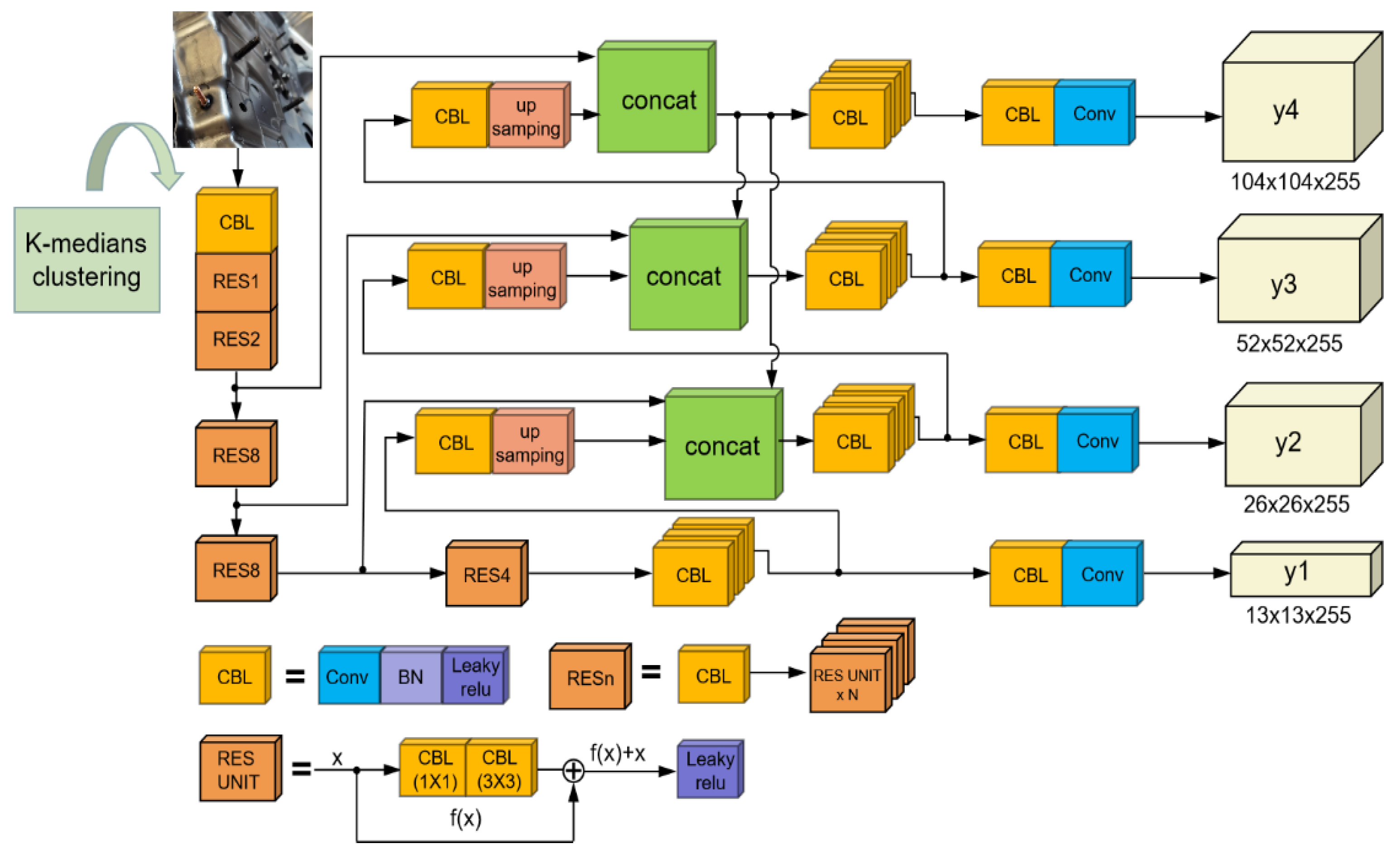
  • In this study, the layer in the prediction model are increased from three to four to more precisely anticipate the workpiece location of the stud. The image pyramid structure is employed to gather stud feature information at various scales, and shallow feature fusion is trained at different sizes to obtain additional stud contour details.
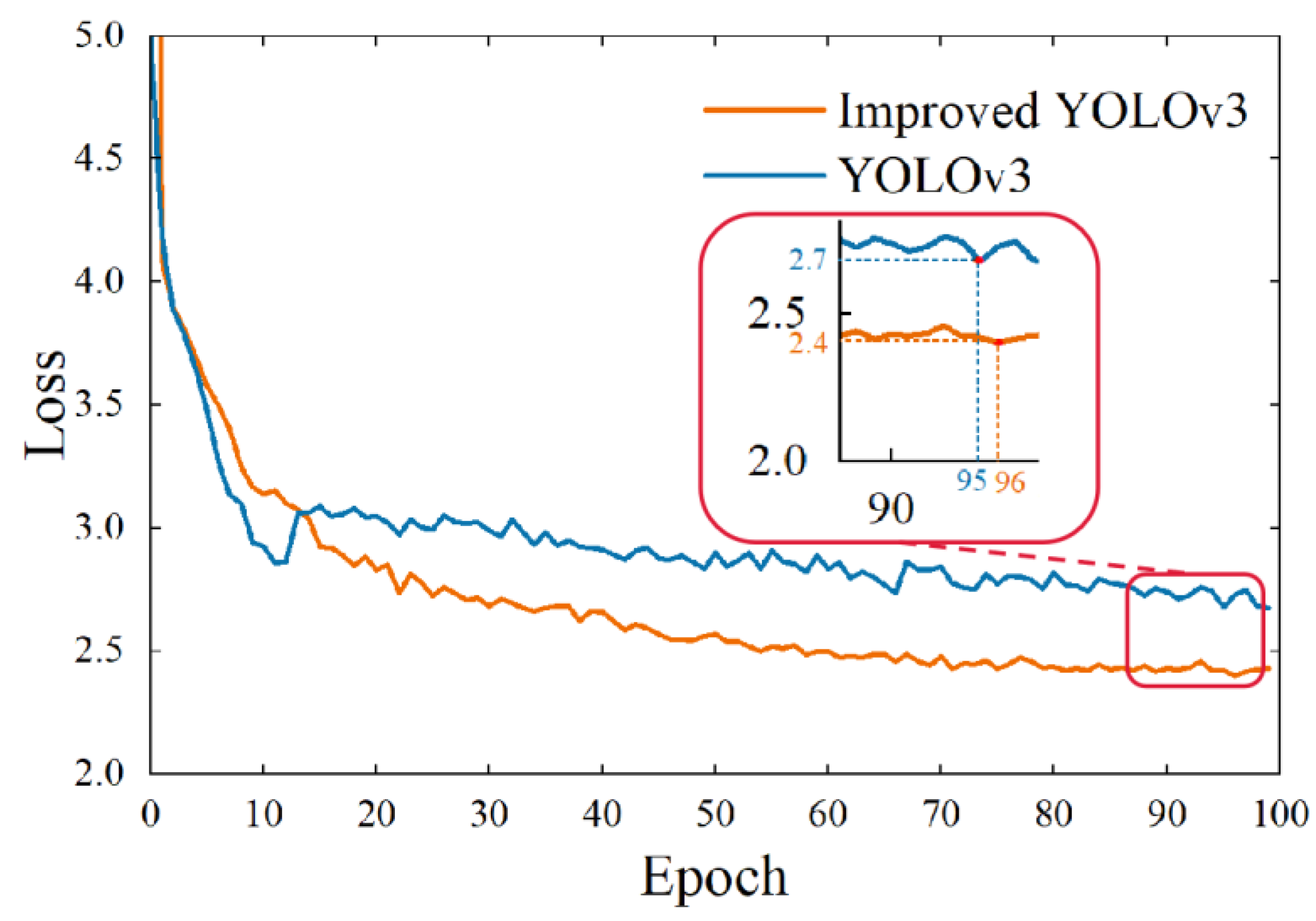
  • The positive and negative sample imbalance problem will reduce the model’s training efficiency and detection accuracy, and it is resolved in this study using the focal loss function. The focal loss function can decrease the weight of the straightforward background classes, allowing the algorithm to concentrate more on detecting the foreground classes and increasing the detection accuracy of studs.
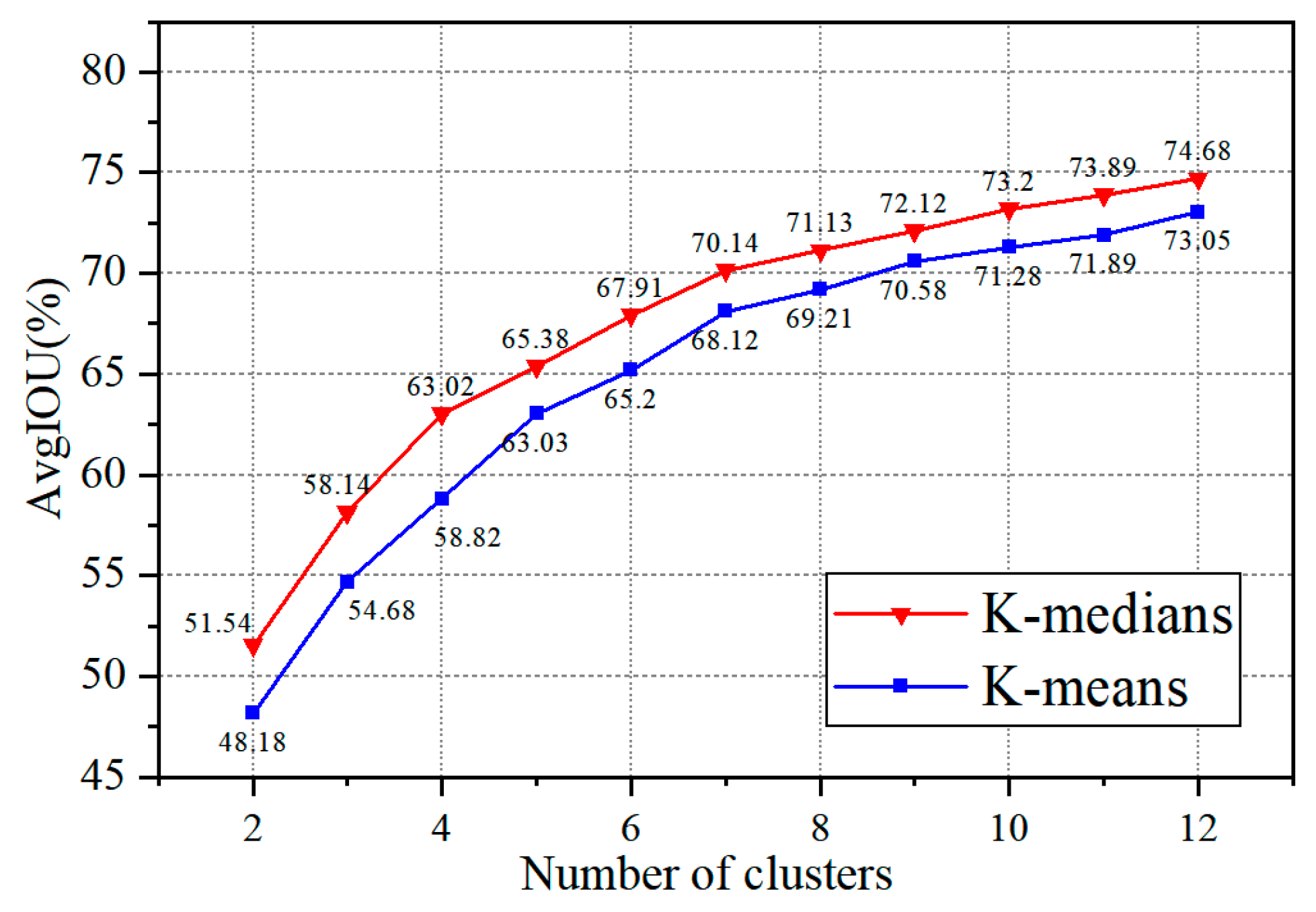
  • A median-based approach is used to solve the problem that the model’s K-means clustering algorithm [18] is sensitive to the initial cluster centers and outliers. The K-medians approach is robust to noisy points or outliers, avoiding the model falling into a local optimum and thus improving the accuracy of the model for stud detection.

2. Improved YOLOv3 Model

This section first describes the conventional YOLOv3 model. Then, the modifications made in this study to increase its performance on stud detection and localization are presented.

2.1. Framework of the YOLOv3 Model

YOLOv3 is a typical single-stage detection technique that transforms the detection problem into a regression problem. It differs from R-CNN, Fast R-CNN, and Faster R-CNN, which are two-stage algorithms that employ a region candidate network to create a sequence of candidate anchor boxes, and it It draws on the idea of feature pyramid network (FPN) to extract features from images at different scales.

2.1.1. Backbone Network of YOLOv3

The backbone network of YOLOv3 is Darknet-53 network [24,25,26], which contains 53 convolutional layers, mainly consisting of 1 × 1 and 3 × 3 convolutional layers. The Darknet-53 network is based on three FPN scales, downsampling by 8×, 16×, and 32×, to generate feature maps corresponding to large, medium, and small scales. The deep small-scale feature maps are upsampled by the FPN module and merged with the shallow large-scale feature maps, as shown in Figure 1. By continually optimizing the step size of the convolution unit and downsampling three times to provide a more detailed small-scale feature map, the Darknet-53 network manages the size of the output feature map. Small-scale feature maps offer more in-depth semantic information because they have a wider perceptual range. Simultaneously, more precise image features are provided by shallow large-scale feature maps.

2.1.2. FPN

The objective of the FPN is to construct feature pyramids out of the hierarchical semantic characteristics of the convolutional network itself [27]. In the YOLOv3 network, the FPN module combines the shallow network position information with the abstract image data recovered from the deep network. For instance, a 26 × 26 feature map is created after being downsampled four times and is then sent to two channels using a sequence of convolutions. Following the upsampling procedure, one channel is fused with the 5× downsampled feature map, and the combined feature map is used as the final prediction output, which is a 26 × 26 output feature map. The final result for the regression prediction is a 52 × 52 feature map produced by the three downsampling operations, which is fused with the other channel handled by the upsampling module. Using the FPN module and top-down approach, the YOLOv3 network produces three scale feature maps of 52 × 52, 26 × 26, and 13 × 13.

2.1.3. Residual Networks

The main difference between YOLOv3 and YOLOv2 is the conversion of the feature extractor network Darknet-19 to Darknet-53 and the extensive introduction of residual networks [28]. In addition, the skip connections of the residual network are added to the network structure. This approach is a good solution to the problem of gradient disappearance or divergence because of the large number of network layers. As shown in Figure 1, RESn represents a residual network module consisting of n residual units. The residual unit contains two convolutional layers with convolutional kernel sizes of 1 × 1 and 3 × 3. By setting the size of the convolutional kernel, the array can be first downdimensioned and then updimensioned, which can reduce the number of computational parameters. In the residual network, the output x of the first channel is processed using two convolutional layers to obtain the value f(x), which is directly added to the value of x in the second channel. This structure ensures that the deep network model converges as much as possible during the training process. The deeper the network layers, the better the learning of object features and the higher the detection accuracy.

2.2. Methods for Improving the YOLOv3 Model

2.2.1. Multiscale Training and Multiscale Prediction

The traditional YOLOv3 model extracts depth features through the upsampling module and fuses feature maps at different scales, thus enabling the network to learn deep and shallow features and eventually predict the feature maps. As shown in Figure 1, the YOLOv3 model takes the input images and predicts feature maps at scales of 52 × 52 × 255, 26 × 26 × 255, and 13 × 13 × 255 after downsampling 8 ×, 16 ×, and 32 ×, respectively. The 32 × downsampled feature maps have a larger sensory field and are suitable for detecting large targets. The 26 × 26 × 255 features, fused by a series of convolutional units and upsampling at the 13 × 13 × 255 scale, have a medium-scale field of view and are suitable for medium-scale target detection. The 52 × 52 × 255 features are similar in principle and ideal for detecting small targets.
Each image is scaled to 416 × 416 on the input side of YOLOv3; however, when the target size is too small, the feature map tends to lose target details during downsampling, and the detection performance degrades. The standard YOLOv3 algorithm will have difficulties identifying stud targets when the pixel area of the stud targets in the automotive workpiece images is less than 9 × 9. Second, while higher-fold downsampling yields a wider perceptual field and allows for the extraction of deeper semantic characteristics, it is easy to lose some target location data, impacting the localization accuracy. The shallow features of the stud weld’s speckle shadow texture, which are critical for target recognition because the target stud has a tiny contour in the workpiece image, should be given greater weight in the feature map fusion. The standard YOLOv3 can recognize small targets using an 8× downsampled feature map, but it cannot properly learn the shallow stud features. This study modifies the YOLOv3 algorithm to address these issues. The specific improvement is as follows: the image size is first adjusted to 608 × 608 on the input side to maintain more stud shape features and the subtleties of the weld joints and weld marks. To train the deep network to understand the shallow properties of the microscopic size of the stud contour, the features acquired from 4×, 8×, and 16× downsampling are blended. Combining the stud weld mark’s speckle shadow texture with deep semantic abstraction characteristics increases the fraction of the external stud features.
Additionally, by connecting the 8× downsampling fusion feature map with the 4× downsampling feature map, this approach increases the number of prediction layers from three to four. The 4× downsampling fusion feature map was employed to find smaller target studs. Figure 2 depicts the altered YOLOv3 structure used in this study.

2.2.2. Improving the Loss Function of YOLOv3

This subsection describes the improvements to the loss function of the YOLOv3 algorithm. Introducing the focal loss function can effectively alleviate the impact of sample category imbalance on the detection algorithm, thus improving its detection accuracy.
The loss function of the traditional YOLOv3 algorithm contains three components: the bounding-box localization bias loss, bounding-box confidence loss, and predicted category probability loss. The bounding-box confidence loss uses binary cross-entropy as the loss function, which takes the following form [29].
L o s s = λ c o o r d i = 0 S 2 j = 0 B I i j o b j [ ( x i x ^ i j ) 2 + ( y i y ^ i j ) 2 ] + λ c o o r d i = 0 S 2 j = 0 B I i j o b j [ ( w i j w ^ i j ) 2 + ( h i j h ^ i j ) 2 ] i = 0 S 2 j = 0 B I i j o b j [ C ^ i j log ( C i j ) + ( 1 C ^ i j ) log ( 1 C i j ) ] λ n o o b j i = 0 S 2 j = 0 B I i j n o o b j [ C ^ i j log ( C i j ) + ( 1 C ^ i j ) log ( 1 C i j ) ] i = 0 S 2 I i j o b j c c l a s s e s [ P ^ i j log ( P i j ) + ( 1 P ^ i j ) log ( 1 P i j ) ]
In Equation (1), λ c o o r d and λ n o o b j represent the loss weights for the coordinates and loss weights without the target confidence, respectively; S 2 represents the total number of input images partitioned into grid cells; B represents the number of predicted bounding boxes for which each grid is responsible; I i j o b j denotes that the j th bounding box of the i th grid cell matches the object in that cell; and I i j n o o b j denotes that the j th bounding box of the i th grid cell does not match the object in that cell. Further, ( x i , y i , w i j , h i j ) and ( x ^ i j , y ^ i j , w ^ i j , h ^ i j ) denote the predicted target box coordinates and true target box coordinates, respectively; ( C i j , P i j ) denotes the confidence level of the predicted target box and class of the predicted target; and ( C ^ i j , P ^ i j ) denotes the confidence level of the real target box and class of the real target.
In the automotive stud inspection task, one image generates many inspection regions, but only a small amount of target stud information is usually contained in these inspection regions. This phenomenon leads to unbalanced sample classes and an excessive number of negative samples, which account for most of the total loss value, ultimately resulting in poor model optimization. To further improve the accuracy of recognition, when designing the loss function for the confidence of the bounding box and the predicted category probability, the proposed method uses the focal loss function [30] to replace the standard cross-entropy loss function. This function makes the model focus more on hard-to-classify samples during training by reducing the weights of the easy-to-classify samples. The focal loss function (FL) is given by the following equation.
F L ( p t ) = α t ( 1 p t ) γ log ( p t ) , p t = { P ,         γ = 1 1 P ,         o t h e r
In Equation (2), ( 1 p t ) γ represents the modulation factor; α t represents the weight hyperparameters that control the positive and negative samples; and γ represents the hyperparameters that manipulate the difficult and easy classification samples.
Integrating Equations (1) and (2), the total loss function of the improved algorithm is as follows.
L o s s = λ c o o r d i = 0 S 2 j = 0 B I i j o b j [ ( x i x ^ i j ) 2 + ( y i y ^ i j ) 2 ] + λ c o o r d i = 0 S 2 j = 0 B I i j o b j [ ( w i j w ^ i j ) 2 + ( h i j h ^ i j ) 2 ] + i = 0 S 2 j = 0 B I i j o b j [ C ^ i j α ( 1 C i j ) γ log ( C i j ) + ( 1 C ^ i j ) α ( C ^ i j ) γ log ( 1 C i j ) ] λ n o o b j i = 0 S 2 j = 0 B I i j n o o b j [ C ^ i j α ( 1 C i j ) γ log C i j + ( 1 C ^ i j ) α ( C ^ i j γ log ( 1 C i j ) ] i = 0 S 2 I i j o b j c c l a s s e s [ P ^ i j α ( 1 P i j ) γ log ( P i j ) + 1 P ^ i j ) α ( P ^ i j ) γ log ( P i j ) ]
For example, the grid prediction feature map size S 2 is 13 × 13, the values of i , j . are 6, 5, respectively; the value of I i j o b j is 1; the value of I i j n o o b j is 0; the values of C ^ i j and P ^ i j are all 1; the width of the feature map W i m a g e is 13 and the height of the feature map H i m a g e is 13, as shown in Figure 3. To overcome the imbalance between positive and negative samples, the hyperparameters α , γ , λ c o o r d , and λ n o o b j are set to values from previous work [17,18,19,31,32], which are 0.95, 8, 5, and 0.5, respectively, applicable to the stud image dataset used in this paper. The set of parameters ( x i , y i , w i j , h i j ) can be solved from the predicted parameters ( t x , t y , t w , t h , C i j , P i j ) of the output feature map and the following equations:
x i = σ ( t x ) , y i = σ ( t y ) , w i j = t w , h i j = t h
where σ is the sigmod activation function.
Then, the true values ( x ^ i j , y ^ i j , w ^ i j , h ^ i j ) can be obtained as follows.
x ^ i j = g x C x , y ^ i j = g y C y , w ^ i j = log ( g w P w ) , h ^ i j = log ( g h P h )
where, p w = a w W i m a g e ; p h = a h H i m a g e ; ( C x , C y ) are the center coordinates of the anchored box, ( a w , a h ) are the width and height of the anchored box, ( g x , g y ) are the center coordinates of the ground truth box, ( g w , g h ) are the width and height of the anchored box, respectively, on the feature map. Joining Equations (4) and (5) and the other parameter values, the loss value is determined.

2.2.3. Improved Clustering Algorithm

The size of the anchor box used for localization directly influences the precision of target identification according to the network detection technique. YOLOv3 employs the K-means clustering technique, which splits the provided set of samples into K (K >= 1) clusters based on the magnitude of the distance between the samples and clusters of targets in the training set based on the sizes of their bounding boxes. The key to the K-means algorithm, which is essentially an unsupervised clustering method based on maximum expectation, is that it reduces the distances between samples within a cluster as much as possible after several repetitions while allowing the distances between samples across clusters to remain large [33]. However, there are two issues with this algorithm [34]: (i) The initial clustering centers affect its sensitivity. This approach produces varying clustering results and localization accuracies when several clustering centers are used. The model gradient descent solution can enter a local optimum because of the random selection of K centroids, resulting in unstable clustering. (ii) Sensitivity to noise and outliers. K-means uses the average of the distances between samples in a cluster as a reference for the next step in calculating the cluster centers. The mean is a measure that is highly susceptible to outliers; even a drastic outlier can move the standard away from most datasets. Therefore, any sample data, especially if it contains noise, can substantially affect the calculation of new points and cause errors. In stud image target detection, a small number of either large or small image targets can exist because of inconsistencies in the in-camera shot height, camera resolution, and the object’s actual size. These inconsistent large and small targets can have an impact on the clustering performance of the K-means algorithm.
By contrast, the median-based K-medians clustering algorithm can effectively improve this situation, and the idea of the improved clustering algorithm is as follows.
The size of the ground truths can be expressed as follows.
θ = { ( B 1 ) , ( B 2 ) , , ( B n 1 ) , ( B n ) } , B i = { W i , H i }
In Equation (6), W i and H i represent the width and height of the i th ground truth; n indicates the quantity of samples.
Firstly, the initial cluster center is determined by randomly choosing a set of samples B i , then computing the distance metric d between each sample in the dataset and c 1 . The maximum value in d becomes the second cluster center c 2 . This is expressed as follows.
d ( B i , c j ) = 1 I O U ( B i , c j ) , i = 1 , 2 , 3 , , n ; j = 1 , 2 , 3 , , k I O U ( B gti , B pdj ) = B gti B pdj B gti B pdj
In Equation (7), B gti represents the i th ground truth; B pdj is the j th prediction frame; and I O U ( B gti , B pdj ) denotes the intersection ratio of the ground truth and center of the bounding box cluster.
The above steps are repeated until K centroids are obtained, and all centroids C are recorded as β = { C 1 , C 2 , , C k 1 , C k } . The distance from each data point to the centroid d [ C i , B J ( C i ) ] is calculated, and that data point is classified as belonging to the class of the closest centroid to achieve local optimization, which is implemented as follows.
d [ C i , B J ( C i ) ] = m i n { d [ C i , B j ( C i ) ] , j = 1 , 2 , 3 k }
In Equation (8), C i denotes the i th random centroid and B j ( C i ) denotes the j th sample that corresponds to the centroid.
Each class of centroids is calculated as a new centroid, B J ( C i + 1 ) , to achieve regional optimality as follows.
B J ( C i + 1 ) = 1 k i = 1 , i k k d [ C i , B j ( C i ) ] , j = 1 , 2 , 3 , , k
The above steps are repeated until each class of centers does not change substantially after several iterations, at which point the optimal global solution has been obtained.
In the proposed method, the operation of finding the mean value in the original K-means clustering algorithm is replaced with finding the median in the K-medians algorithm. On the one hand, the median is highly robust to noisy points or outliers, avoiding the effect of anomalous target sizes and thus improving the target detection accuracy. On the other hand, the inference procedure of the YOLOv3 network is unrelated to the K-medians clustering method. The specific approach is shown in Figure 2. First, 12 more appropriate anchor box sizes with the same role as the network prior frame are generated by the K-medians clustering algorithm. Training the model based on the size of the anchor boxes implies that it does not typically impose any computational drain on the model and reduces the complexity of the algorithm during detection. The improved clustering algorithm facilitates the accurate localization of small targets such as studs.

2.2.4. Optimized Convolution Units

In a convolutional neural network, the input distribution of all the hidden layers changes as the parameters of the neurons in the previous layer change. This leads to problems such as slower forward propagation of the network, inability to use dynamically changing learning rates, and sensitivity of network training to initialization parameters. The BN layer, located between the convolutional and activation layers in the CBL (Convolutional, batch normalization and leaky relu layer) module of the convolutional unit, improves the ability of the trained model to fit new samples, reduces gradient disappearance, and facilitates model convergence. Therefore, the BN layer is widely used in the network training process to accelerate the convergence of the model and solve the overfitting problem [35].
However, adding a BN layer to the network forward propagation process results in an increase in computation, which leads to a decrease in the forward inference speed and consumes more memory resources. To overcome these disadvantages, this section describes how the proposed method incorporates the BN layer into the convolutional layer to reduce the memory resources required for forward propagation of the network and to improve the target detection speed of the model without affecting the effectiveness of target detection. The BN layer is calculated as follows.
F ^ i , j = W B N × F i , j + b B N
In Equation (10), F ^ i , j denotes the normalized result; W B N represents the BN layer weight; b B N represents the BN layer bias; and F i , j represents the feature map processed by the convolutional layer, which is represented as follows.
F i , j = W c o n v × f i , j + b c o n v
In Equation (11), W c o n v represents the weight matrix of the convolutional layer; f i , j represents the convolution layer; b c o n v represents the bias of the convolutional layer.
The BN layer was incorporated into the convolution layer in the following manner.
F ^ i , j = W B N × ( W c o n v × f i , j + b c o n v ) + b B N = ( W B N × W c o n v ) × f i , j + ( W B N × b c o n v + b B N ) = W × f i , j + b
In Equation (12), W represents W B N × W c o n v and b represents W B N × b c o n v + b B N .

3. Experiments and Results

This section evaluated the stud detection algorithm proposed in this paper using images of studs from automotive workpieces.

3.1. Stud Dataset

In this evaluation, 4000 stud images were collected from the site of an automotive production line. The images contain different types of stud targets in near and far views, and some data samples are shown in Figure 4. As shown in Figure 4, there is significant background noise interference when automotive workpieces are inspected on the production line, such as jigs, protective fences, and other auxiliary equipment in the work section. In addition, in some views, stud targets are difficult to identify because they occupy a small area in the field of view. Real-time detection of stud targets on a production line is hence challenging.

3.2. Details of the Implementation

The entire study dataset was divided into a training set and a test set using a ratio of 8:2. The improved YOLOv3 algorithm was implemented using the PyTorch framework [36], and the experimental environment is summarized in Table 1.
The input image size is 608 × 608, as required by the proposed algorithm. The original data were augmented and extended by flip transforms, random trimming, translation, and saturation and hue adjustments. Table 2 lists the initial parameter settings for model training. The number of input training images per batch was 16. The number of training epochs was 100.
Figure 5 compares the effect of the change in loss values when training the model in this study (orange) and the original YOLOv3 model (blue) using the stud image dataset. The horizontal coordinates indicate the number of training epochs, and the vertical coordinates indicate the total loss value. Figure 5 shows that the YOLOv3 model starts to converge at about the 80th epoch. Although the initial loss value of the model proposed in this paper is significantly larger than that when the YOLOv3 model is adopted, Focal Loss is used to calculating the error when designing the bounding box confidence loss function and predicted category probability. Therefore, after 96 times of training, its loss value converges to about 2.4. It is lower than 2.7 of the loss value of the original YOLOv3 model. To sum up, when the model proposed in this paper is adopted, the total Loss obtained by training is smaller. The model in this paper has better convergence.

3.3. Evaluation Methods

The average intersection over union (AvgIOU) [37], precision (P), and recall (R) were used to evaluate the performance of stud detection after stud target prediction [14,38,39]. The AvgIOU is a standard evaluation metric used to quantify the precision of target identification by employing the AvgIOU between the prior frame created by the model and the ground truth of the training set to evaluate the proposed clustering. The performance of the proposed clustering method is assessed using the AvgIOU between the prior frame created by the model and the ground truth of the training set. The proposed method has the same nine predefined initial frames as the original YOLOv3, and the robustness of the algorithm localization is assessed by calculating the overlap between the prior frames and real samples.
The precision contains a percentage of true positives (TP) and false positives (FP). Recall is the probability of the accuracy of the detected workpiece studs [40]. The precision (P) and recall (R) are defined as follows.
P = TP TP + FP
R = TP TP + FN
Average precision (AP) and mean average precision (mAP) are the integral of the accuracy recall curve and average accuracy of all types of studs on the workpiece, respectively [41]. These indicators are expressed as follows.
A P = 0 1 P ( R ) d R
mAP = 1 N i = 1 N A P i
Here, N is the number of workpiece stud types; A P i represents the average precision value of the i th workpiece stud types.
In an industrial production environment, the speed of detection of a model is a critical evaluation metric that is usually expressed as the F P S .
F P S = N u m F i g u r e T o t a l T i m e
In Equation (17), N u m F i g u r e represents the number of images detected, and T o t a l T i m e represents the total time spent detecting the images.
The F 1 value is the summed average of precision and recall. Neither precision nor recall alone can be used as an indicator of a model’s performance, and hence the F 1 value is used because it is compatible with precision and recall.
F 1 = 2 × p r e c i s i o n × r e c a l l p r e c i s i o n + r e c a l l

3.4. Experimental Results and Analysis

3.4.1. Anchor Box Optimization Experiments

The AvgIOU values were compared for the proposed clustering approach with those of the K-means method using the automotive workpiece stud image dataset. The results are presented in Table 3. As the number of cluster centers increases, the two algorithms’ AvgIOU values increase, with the critical point being when the cluster centers are equal to seven. When K is less than seven, the slope of the AvgIOU curve is more significant, and when K more than seven, the curve gradually flattens out, as shown in Figure 6. This is because, as the number of clustering centers increases, there is a better fit between the a priori anchor box generated by the model and the ground truth box. However, it is essential to note that too many clustering centers increase the computational complexity of the algorithm during forward propagation and backpropagation. In practice, when the output layer of the network structure model consists of four nodes, 12 clustering centers are required to meet the detection requirements. When the number of clustering centers is 12, the AvgIOU values of the proposed algorithm and the YOLOv3 algorithm are 74.68% and 73.05%, respectively. The new clustering method applied in the proposed algorithm improves the results of the YOLOv3 algorithm by 1.63%. Therefore, the proposed clustering method is effective.

3.4.2. Ablation Experiments

Ablation experiments were performed in this study for comparative analysis and to show the efficacy of each proposed module. The YOLOv3 model was used as the baseline for the comparison analysis, with the YOLOv3 model’s structure improved by the addition of multiscale prediction branches, the use of the K-medians technique for clustering, and the optimization of the original loss function. Additionally, headless studs are difficult to identify because they are small targets. Various enhancement techniques were evaluated with an Intersection over Union (IOU)threshold of 0.5, and the experimental findings are compared in Table 4.
The model proposed in this study achieved an mAP of 80.42%, which is a 3.26% improvement in the mAP values of the original YOLOv3 algorithm. The AP values of the improved YOLOv3 for detecting both types of studs were improved by 2.72% and 3.8%, respectively, compared with the results of the original YOLOv3 model. This demonstrates the superior detection capability of the proposed model when detecting small targets such as studs. Table 3 reveals that the mAP value is improved by 2.12% when multiscale branches are added for prediction. The 3.04% increase in AP in the detection of headless studs implies that the improved model is better at capturing information regarding small targets in the original image. The reason for this result is that the proposed model has an enhanced ability to extract detailed feature information from the backbone network by predicting targets at multiple scales, particularly by effectively using feature information from the shallow layers of the image.
When clustering using the K-medians algorithm, the mAP value increases to 77.72%. This is attributed to the fact that the proposed clustering algorithm selects better clustering centers in the initial stage, which not only reduces the effect of noise points on the size of the anchor frame but also reduces unnecessary fitting behavior and increases the likelihood that the algorithm will avoid falling into a local optimum. Comparing the experimental results of the original loss function using the focus loss function alone and YOLOv3, with the former having an mAP value of 78.18% and the latter having an mAP value of 77.16%, which is a favorable result. In the focus loss function, as the number of iterations increases, the modulation factor equalizes the weights of complex and easy-to-classify samples and reduce the consequences of the easy-to-classify samples, allowing the model to focus more on the hard-to-classify examples during training. When the network model extracts the stud feature information, the grid weight for the stud object is considerable, thus enhancing the target feature information. The grid weight for the background is smaller, which reduces the impact of complex background features and ultimately reduces the effect of the samples on the total loss.

3.4.3. Experimental Analysis of Different Models

Comparative experiments on the proposed model and different target detection models (DPM(Deformable Parts Model), R-CNN, Faster R-CNN, SSD, and YOLOv3) were conducted on the self-built stud dataset. The primary analysis metrics were the AP values, mAP values, and detection speed (FPS) of the different algorithms for the two types of stud detection. The experimental results are listed in Table 5. Compared with the DPM, R-CNN, Faster R-CNN, SSD, and YOLOv3 models, the proposed method improved the mAP values by 17.84%, 35.75%, 8.47%, 17.69%, and 3.26%, respectively. The modified approach substantially improves the recognition accuracy for studs when compared with the R-CNN and Faster R-CNN algorithms. It also has a significant advantage in terms of detection speed because the proposed method is a single-stage detection algorithm that does not use a complex region proposal network but instead treats the detection process as a regression problem. When compared with YOLOv3, the improved method has a 0.05-s disadvantage in terms of detection speed. However, the proposed model has a better characterization of the target and is better able to find stud targets in a complex production line background environment while satisfying real-time requirements.
To further evaluate the advantages and efficiency of the improved method for small-target detection, comparing the experimental results obtained by the mainstream methods when detecting small studs (headless studs), as shown in Table 6. The AP values of the four models for the small-stud dataset are 70.39%, 58.25%, 75.61%, and 79.41%, respectively. The AP values of the YOLOv3 model are higher than those of the SSD and Faster R-CNN models, and the method achieves an improvement of 3.8% over the YOLOv3 model.
The precision and recall (P–R) curve plots for each method are shown in Figure 7. The vertical coordinates indicate the change in precision, and the horizontal coordinates indicate the change in recall. The larger the area under the P-R curve, the better the detection performance of the model. As shown in Figure 7, the precision of the SSD model decreases substantially as the recall rate increases. The precision of Faster R-CNN reaches 86% when the recall rate reaches 64% and decreases substantially as the recall rate continues to increase. Compared to the first two models, the precision of the YOLOv3 model slowly decreased as the recall rate increased. When the recall rate reached 74%, the model had a precision rate of 90.2%, but it also showed a somewhat decreasing trend. In contrast, the method in this paper plots the P-R graph curve with a larger area enclosed by the axes and performs better in terms of recall and precision, reaching 91% precision when the recall rate is 80%, while the method in this paper is significantly higher than other algorithms in terms of F1 values. In summary, our method can identify small targets, such as studs on automotive workpieces, and, in practice, better meets the industry’s requirements for stud detection algorithms in real-time.

3.4.4. Analysis of the Experimental Results

In this study, images were selected from the test dataset for the target detection experiments. The detection results were compared with those of the Faster R-CNN, SSD, and YOLOv3 algorithms to qualitatively evaluate the detection performance of the proposed method for automotive workpiece studs. The results are shown in Figure 8a–c. In Figure 8a, all four algorithms can detect and locate studs when there are two types of studs in the image, but the Faster R-CNN algorithm has three missed detections for headless studs and one false detection for hexagonal studs. The SSD algorithm had five missed and two false detections. The YOLOv3 algorithm has two missed detections and one erroneous detection. The proposed model has only one missed detection. Comparing the experimental results in Figure 8b, the Faster R-CNN and SSD models have substantially lower detection performance for small studs and cannot effectively complete the identification in a long-range view with complex background features. The YOLOv3 model obtains fewer missed and false detections for both types of studs, but still suffers from missed detections of headless studs. Comparing the YOLOv3 model with the proposed model, the latter is more likely to capture small target features, such as automotive workpiece studs, effectively reducing the problems of the YOLOv3 model. Figure 8c reveals that the proposed model has the best IOU for detection and more accurate localization than the other three algorithms. The above analysis demonstrates that the improved model has a high detection accuracy for both types of automotive studs and performs well in the close-range views. Although there are some missed detections in the long-range view, the improved model has better multiscale stud recognition and positioning accuracy than the other algorithms.

4. Discussion and Conclusions

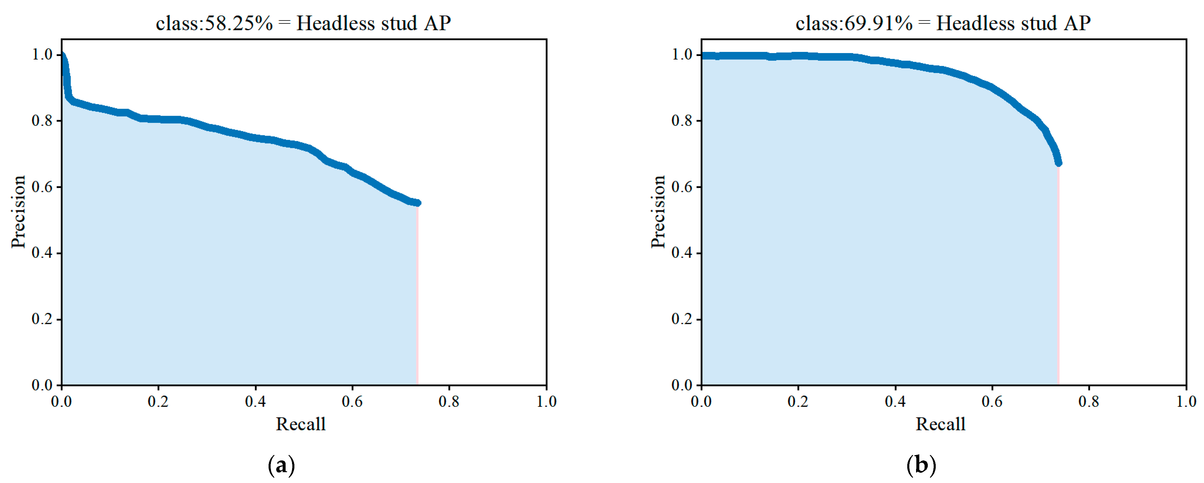
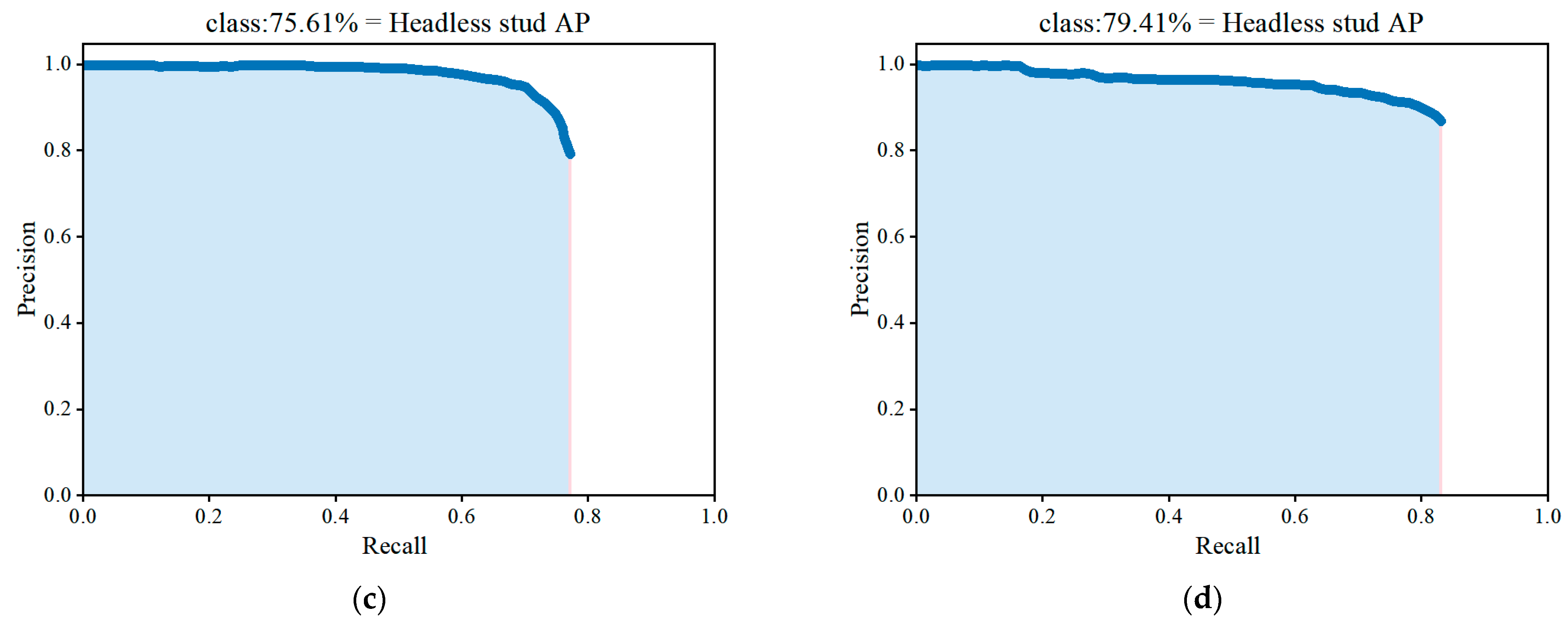
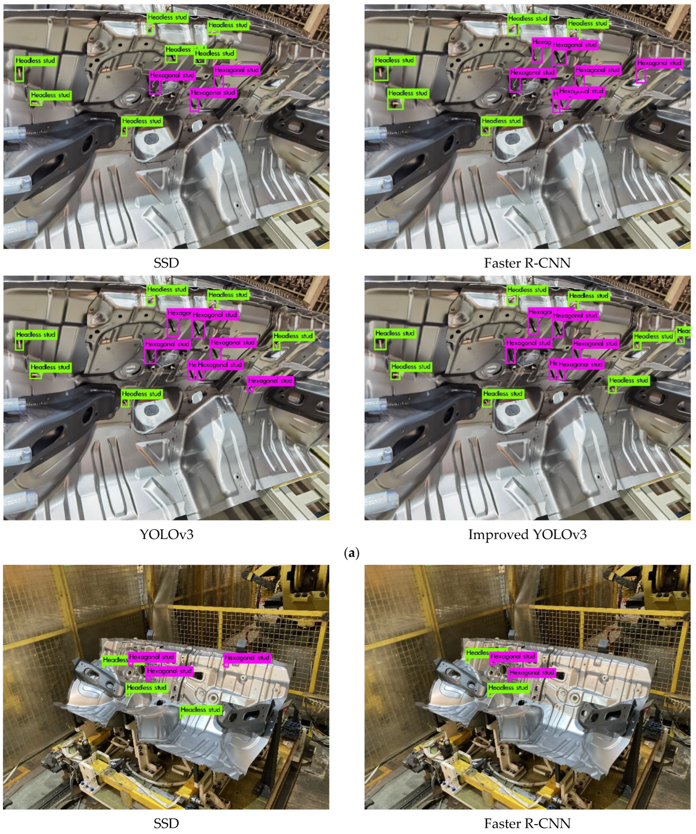
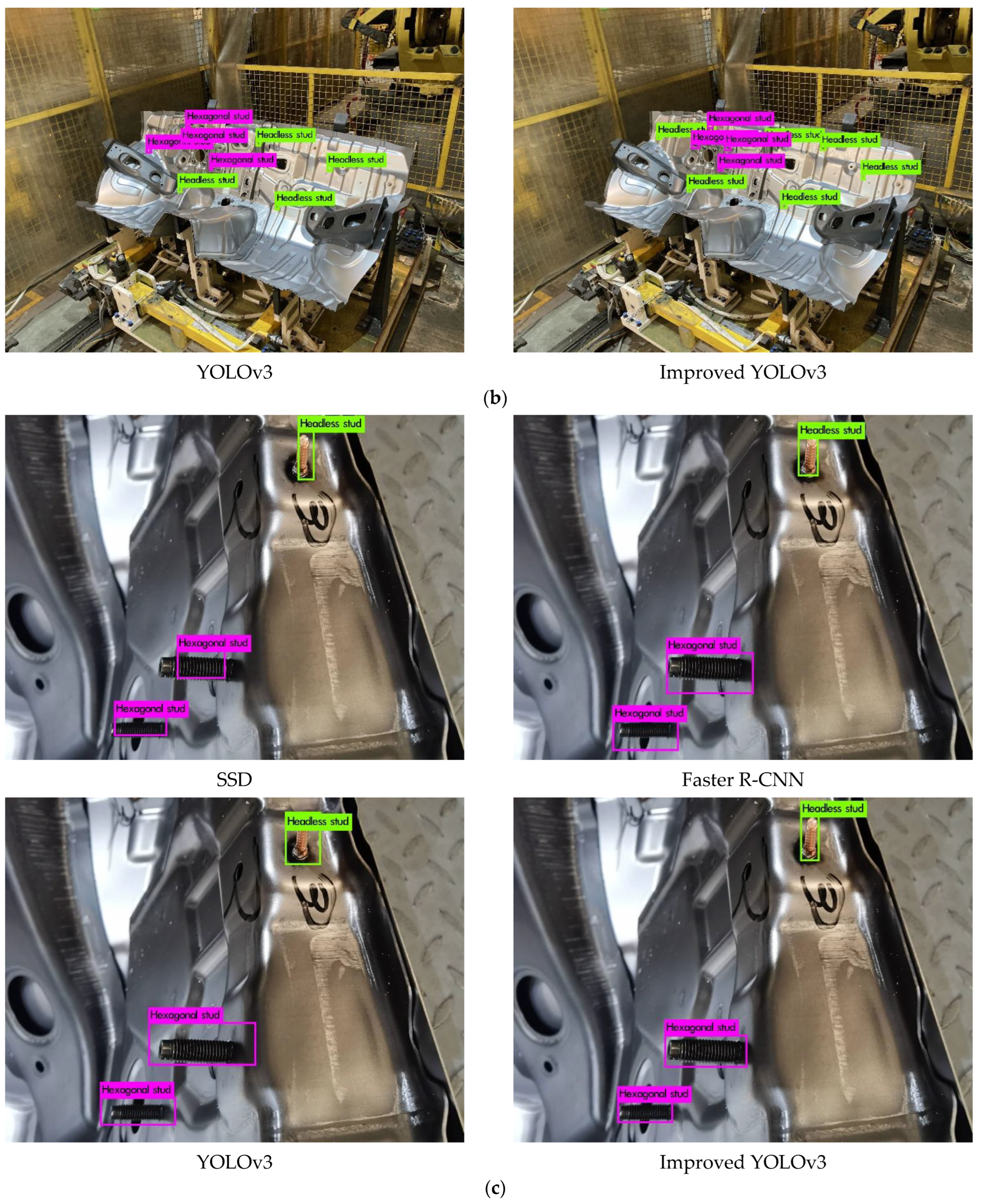
This study proposed a stud leakage detection algorithm based on an improved YOLOv3 model, which was designed to detect studs in automotive workpieces. Firstly, increased the prediction layers of the model structure was increased from three layers to four layers, extracting more details of the stud contours. Secondly, the focal loss function was introduced into the algorithm to solve the positive and negative sample imbalance problem. Finally, an improved K-median clustering method instead of K-means in the original algorithm was used to reduce the adverse effects of noisy points or outliers and prevent the algorithm from falling into local optima and overall oscillations to some extent. The experimental results showed that the modified clustering algorithm achieved an AvgIOU value of 74.68% on the stud dataset, which is 1.63% higher than that of the previous work. The overall algorithm mAP value is 80.3%, compared to 77%, 71.95%, and 62.73% for the conventional YOLOv3, Faster R-CNN, and SSD, respectively. The improved method can achieve a detection speed of 0.32 s to process an image, meeting the requirements of real-time stud detection. The series of experiments conducted in this study demonstrated the effectiveness of the proposed method for stud-detection tasks.
However, in this study, there is still the problem of false detection due to inadequate feature extraction in the case of insufficient light or backlight.In addition, the method still has room for improvement regarding detection speed.Therefore, the next step should improve the algorithm robustness in low-light scenes by adding an attention mechanism, and increase detection speed by reducing the algorithm complexity using model distillation techniques.

Author Contributions

Conceptualization, P.C. and K.L.; methodology, P.C. and K.L.; software, H.F. and P.C.; validation, P.C., K.L. and H.F.; formal analysis, J.Z.; investigation, K.L. and H.F.; resources, K.L., H.F. and J.Z.; data curation, K.L.; writing—original draft preparation, P.C. and K.L.; writing—review and editing, H.F. and J.Z.; visualization, P.C. and K.L.; supervision, H.F. and J.Z.; project administration, K.L.; funding acquisition, P.C. All authors have read and agreed to the published version of the manuscript.

Funding

This research was funded by the Central Government Guides Local Science and Technology Development Foundation Projects (grant no.ZY19183003), Guangxi Key Research and Development Project (grant no.AB20058001).

Institutional Review Board Statement

Not applicable.

Informed Consent Statement

Not applicable.

Data Availability Statement

Not applicable.

Conflicts of Interest

The authors declare no conflict of interest.

References

  1. Ahmad, H.M.; Rahimi, A. Deep learning methods for object detection in smart manufacturing: A survey. J. Manuf. Syst. 2022, 64, 181–196. [Google Scholar] [CrossRef]
  2. Auerswald, M.M.; von Freyberg, A.; Fischer, A. Laser line triangulation for fast 3D measurements on large gears. Int. J. Adv. Manuf. Technol. 2019, 100, 2423–2433. [Google Scholar] [CrossRef]
  3. Li, J.; Zhou, Q.; Li, X.; Chen, R.; Ni, K. An improved low-noise processing methodology combined with PCL for industry inspection based on laser line scanner. Sensors 2019, 19, 3398. [Google Scholar] [CrossRef] [Green Version]
  4. Guo, C.; Xu, C.; Hao, J.; Xiao, D.; Yang, W. Ultrasonic non-destructive testing system of semi-enclosed workpiece with dual-robot testing system. Sensors 2019, 19, 3359. [Google Scholar] [CrossRef] [Green Version]
  5. Lee, S.; Chang, L.-M.; Skibniewski, M. Automated recognition of surface defects using digital color image processing. Autom. Constr. 2006, 15, 540–549. [Google Scholar] [CrossRef]
  6. Kumar, J.; Srivastava, S.; Anand, R.S.; Arvind, P.; Bhardwaj, S.; Thakur, A. GLCM and ANN based approach for classification of radiographics weld images. In Proceedings of the 2018 IEEE 13th International Conference on Industrial and Information Systems (ICIIS), Rupnagar, India, 1–2 December 2018; pp. 168–172. [Google Scholar]
  7. Zhang, J.; Guo, Z.; Jiao, T.; Wang, M. Defect detection of aluminum alloy wheels in radiography images using adaptive threshold and morphological reconstruction. Appl. Sci. 2018, 8, 2365. [Google Scholar] [CrossRef] [Green Version]
  8. Shi, T.; Kong, J.Y.; Wang, X.D.; Liu, Z.; Zheng, G. Improved Sobel algorithm for defect detection of rail surfaces with enhanced efficiency and accuracy. J. Cent. South Univ. 2016, 23, 2867–2875. [Google Scholar] [CrossRef]
  9. Hazarika, A.; Sistla, P.; Venkatesh, V.; Choudhury, N. Approximating CNN computation for plant disease detection. In Proceedings of the 2022 IEEE 46th Annual Computers, Software, and Applications Conference (COMPSAC), Los Alamitos, CA, USA, 27 June–1 July 2022; pp. 1117–1122. [Google Scholar]
  10. Li, J.; Chen, Y.Q.; Li, W.Y.; Gu, J.A. Balanced-YOLOv3: Addressing the imbalance problem of object detection in PCB assembly scene. Electronics 2022, 11, 1183. [Google Scholar] [CrossRef]
  11. Liu, B.L.; Luo, H.; Wang, H.T.; Wang, S.X. YOLOv3_ReSAM: A small-target detection method. Electronics 2022, 11, 1635. [Google Scholar] [CrossRef]
  12. Liu, H.; Yan, Y.; Song, K.; Chen, H.; Yu, H. Efficient optical measurement of welding studs with normal maps and convolutional neural Network. IEEE Trans. Instrum. Meas. 2021, 70, 1–14. [Google Scholar] [CrossRef]
  13. Liu, L.; Ouyang, W.L.; Wang, X.G.; Fieguth, P.; Chen, J.; Liu, X.W.; Pietikainen, M. Deep learning for generic object detection: A survey. Int. J. Comput. Vis. 2020, 128, 261–318. [Google Scholar] [CrossRef] [Green Version]
  14. Ren, S.; He, K.; Girshick, R.; Sun, J. Faster r-cnn: Towards real-time object detection with region proposal networks. IEEE Trans. Pattern Anal. Mach. Intell. 2017, 39, 1137–1149. [Google Scholar] [CrossRef] [PubMed] [Green Version]
  15. Wang, K.; Wang, Y.; Zhang, S.; Zhang, J.; Sun, S. Automatic label welding robot system for bundled rebars. IEEE Access 2021, 9, 160072–160084. [Google Scholar] [CrossRef]
  16. Zhong, S.; Xu, W.; Zhang, T.; Chen, H. Identification and depth localization of clustered pod pepper based on improved Faster R-CNN. IEEE Access 2022, 10, 93615–93625. [Google Scholar] [CrossRef]
  17. Redmon, J.; Divvala, S.; Girshick, R.; Farhadi, A. You only look once: Unified, real-time object detection. In Proceedings of the IEEE Conference on Computer Vision and Pattern Recognition, Las Vegas, NV, USA, 26 June 2016; pp. 779–788. [Google Scholar]
  18. Redmon, J.; Farhadi, A. YOLO9000: Better, faster, stronger. In Proceedings of the IEEE Conference on Computer Vision and Pattern Recognition, Honolulu, HI, USA, 22–25 July 2017; pp. 7263–7271. [Google Scholar]
  19. Redmon, J.; Farhadi, A. Yolov3: An incremental improvement. arXiv 2018, arXiv:1804.02767. [Google Scholar]
  20. Chang, L.A.; Chen, Y.T.; Wang, J.H.; Chang, Y.L. Modified YOLOv3 for ship detection with visible and infrared images. Electronics 2022, 11, 739. [Google Scholar] [CrossRef]
  21. Li, H.; Liu, L.Z.; Du, J.; Jiang, F.; Guo, F.; Hu, Q.L.; Fan, L. An improved YOLOv3 for foreign objects detection of transmission lines. IEEE Access 2022, 10, 45620–45628. [Google Scholar] [CrossRef]
  22. Chen, X.; Lv, J.; Fang, Y.; Du, S. Online detection of surface defects based on improved YOLOV3. Sensors 2022, 22, 817. [Google Scholar] [CrossRef]
  23. Zaidi, S.S.A.; Ansari, M.S.; Aslam, A.; Kanwal, N.; Asghar, M.; Lee, B. A survey of modern deep learning based object detection models. Digital Signal Process. 2022, 126, 103514. [Google Scholar] [CrossRef]
  24. Chen, L.; Xiong, W.; Yang, S.; Zhang, Z. Research on Recognition Technology of Transformer Oil Leakage Based on Improved YOLOv3. In Proceedings of the 2020 International Conference on Computer Information and Big Data Applications (CIBDA), Guiyang, China, 17–19 April 2020; pp. 454–458. [Google Scholar]
  25. Chen, L.; Zhou, Y.; Zhou, H.; Zu, J. Detection of Polarizer Surface Defects Based on an Improved Lightweight YOLOv3 Model. In Proceedings of the 2022 4th International Conference on Intelligent Control, Measurement and Signal Processing (ICMSP), Hangzhou, China, 8–10 July 2022; pp. 138–142. [Google Scholar]
  26. Arvind, C.S.; Aditya, K.; Keerthan, H.S.; Farhan, M.; Asha, K.N.; Patil, S.S. Non-Invasive Multistage Fruit Grading Application with User Recommendation system. In Proceedings of the 2022 IEEE International Conference on Electronics, Computing and Communication Technologies (CONECCT), Bangalore, India, 8–10 July 2022; pp. 1–6. [Google Scholar]
  27. Lin, T.-Y.; Dollár, P.; Girshick, R.; He, K.; Hariharan, B.; Belongie, S. Feature pyramid networks for object detection. In Proceedings of the IEEE Conference on Computer Vision and Pattern Recognition, Honolulu, HI, USA, 22–25 July 2017; pp. 2117–2125. [Google Scholar]
  28. He, K.; Zhang, X.; Ren, S.; Sun, J. Deep residual learning for image recognition. In Proceedings of the IEEE Conference on Computer Vision and Pattern Recognition, Las Vegas, NV, USA, 26 June 2016; pp. 770–778. [Google Scholar]
  29. de Boer, P.-T.; Kroese, D.P.; Mannor, S.; Rubinstein, R.Y. A tutorial on the cross-entropy method. Ann. Oper. Res. 2005, 134, 19–67. [Google Scholar] [CrossRef]
  30. Lin, T.Y.; Goyal, P.; Girshick, R.; He, K.; Dollár, P. Focal loss for dense object detection. In Proceedings of the IEEE international conference on computer vision, Honolulu, HI, USA, 22–25 July 2017; pp. 2980–2988. [Google Scholar]
  31. Daogang, P.; Ming, G.; Danhao, W.; Jie, H. Anomaly identification of critical power plant facilities based on YOLOX-CBAM. In Proceedings of the 2022 Power System and Green Energy Conference (PSGEC), Shanghai, China, 25–27 August 2022; pp. 649–653. [Google Scholar]
  32. Cuellar, A.; Mahalanobis, A. Detection of small moving targets in cluttered infra-red imagery. IEEE Trans. Aerosp. Electron. Syst. 2022, AES-1, 1–19. [Google Scholar] [CrossRef]
  33. Kanungo, T.; Mount, D.M.; Netanyahu, N.S.; Piatko, C.D.; Silverman, R.; Wu, A.Y. An efficient k-means clustering algorithm: Analysis and implementation. IEEE Trans. Pattern Anal. Mach. Intell. 2002, 24, 881–892. [Google Scholar] [CrossRef]
  34. Ahmed, M.; Seraj, R.; Islam, S.M.S. The k-means algorithm: A comprehensive survey and performance evaluation. Electronics 2020, 9, 1295. [Google Scholar] [CrossRef]
  35. Ioffe, S.; Szegedy, C. Batch normalization: Accelerating deep network training by reducing internal covariate shift. In Proceedings of the International Conference on Machine Learning, Lille, France, 6–11 July 2015; pp. 448–456. [Google Scholar]
  36. Fey, M.; Lenssen, J.E. Fast graph representation learning with PyTorch Geometric. arXiv 2019, arXiv:1903.02428. [Google Scholar]
  37. Liu, M.; Tang, L.; Li, Z. Real-Time object detection in UAV vision based on neural processing units. In Proceedings of the 2022 IEEE 6th Information Technology and Mechatronics Engineering Conference (ITOEC), Chongqing, China, 4–6 March 2022; Volume 6, pp. 1951–1955. [Google Scholar]
  38. Yue, X.; Li, H.; Shimizu, M.; Kawamura, S.; Meng, L. YOLO-GD: A deep learning-based object detection algorithm for rmpty-dish recycling robots. Machines 2022, 10, 294. [Google Scholar] [CrossRef]
  39. Liu, W.; Anguelov, D.; Erhan, D.; Szegedy, C.; Reed, S.; Fu, C.-Y.; Berg, A.C. Ssd: Single shot multibox detector. In Computer Vision—ECCV 2016, Proceedings of the 14th European Conference on Computer Vision, Amsterdam, The Netherlands, 11–14 October 2016; Springer: Cham, Switzerland; pp. 21–37.
  40. Haixia, M.; Zhongxing, L.; Na, S.; Zhe, Z. Research on defect identification of key components of transmission line based on deep learning. In Proceedings of the 2022 Power System and Green Energy Conference (PSGEC), Shanghai, China, 25–27 August 2022; pp. 969–973. [Google Scholar]
  41. Liu, C.Y.; Wu, Y.Q.; Liu, J.J.; Sun, Z. Improved YOLOv3 network for insulator detection in aerial images with diverse background interference. Electronics 2021, 10, 771. [Google Scholar] [CrossRef]
Figure 1. YOLOv3 algorithm network structure.
Electronics 11 03430 g001
Figure 2. Improved YOLOv3 algorithm network structure.
Electronics 11 03430 g002
Figure 3. Predicted feature map for a 13 × 13 grid (The red dashed rectangular box is the anchoring box. The yellow rectangular box is ground truth box. The blue box represents the grid in row i and column j).
Electronics 11 03430 g003
Figure 4. Studs on automotive workpieces.
Electronics 11 03430 g004
Figure 5. Loss values of YOLOv3 and the improved YOLOv3.
Electronics 11 03430 g005
Figure 6. AvgIOU of the K-means method and K-medians method on the studs dataset.
Electronics 11 03430 g006
Figure 7. P-R curves of four methods on the studs dataset. (a) SSD; (b) Faster R-CNN; (c) YOLOv3; (d) Improved YOLOv3.
Electronics 11 03430 g007aElectronics 11 03430 g007b
Figure 8. Comparison of partial target detection results of the four models on three images. (a) Close distance detection; (b) long distance detection; (c) IOU comparsion.
Electronics 11 03430 g008aElectronics 11 03430 g008b
Table 1. Experimental configuration and parameters.
ConfigurationParameter
CPUIntel Core 10,900
GPUNVIDIA RTX 3090 ti 24 G
RAM32 G
Operating systemWindows 10
Table 2. Initialization parameters of training.
AlgorithmImage SizeBatch SizeMomentumLearning RateDecay
Improved YOLOv3608 × 608160.90.0010.0005
Table 3. Comparison of the AvgIOU (%) results from the two clustering method on the studs dataset.
AlgorithmK
23456789101112
K-means48.1854.6858.8563.0365.2068.1269.2170.5871.2871.8973.05
K-medians51.3458.1463.0265.3867.9170.1471.1372.1273.2073.8974.68
Table 4. Experiments with different modules on the studs dataset. S: multiscale training and multiscale prediction, K: K-medians clustering algorithm, F: focal loss function, @: IOU threshold value.
ModelMultiscaleK-MediansFocal LossAverage Precision (AP @ 0.5) (%)mAP (%)
Hexagonal StudHeadless Stud
YOLOv3×××78.7075.6177.16
YOLOv3 + S××79.9178.6579.28
YOLOv3 + K××79.5275.9177.72
YOLOv3 + F××79.7276.6478.18
YOLOv3 + S + K×80.5179.0179.76
YOLOv3 + S +F×80.7679.2480.00
Improved YOLOv381.4279.4180.42
Table 5. Results of several algorithms’ detection on the studs dataset. @: IOU threshold value.
ModelAverage Precision (AP @ 0.5) (%)mAP (%)Detection Speed (s)
Hexagonal StudHeadless Stud
DPM70.5354.6262.580.61
R-CNN50.2539.0644.67- -
Faster R-CNN73.5170.3971.950.86
SSD67.2158.2562.730.42
YOLOv378.7075.6177.160.27
Improved YOLOv381.4279.4180.420.32
Table 6. Comparison of test results of four models on headless stud dataset.
ModelPrecision (%)Recall (%)AP (%)F1 (%)
Faster R-CNN81.2468.3270.3974.22
SSD55.1867.6558.2560.78
YOLOv388.3474.9175.6181.07
Improved YOLOv389.2081.0779.4184.94
Publisher’s Note: MDPI stays neutral with regard to jurisdictional claims in published maps and institutional affiliations.

