
An Aircraft Trajectory Prediction Method Based on Trajectory Clustering and a Spatiotemporal Feature Network


Abstract
:1. Introduction
- (1)
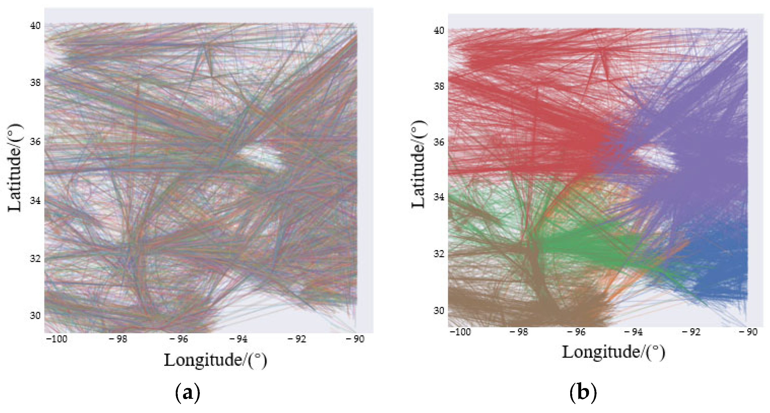
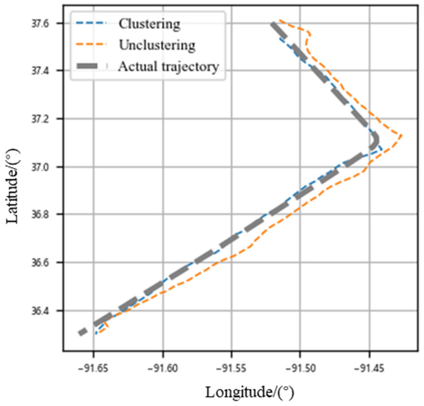
- Based on a large number of real trajectory data, we used the method of trajectory clustering to find out the hidden route rules in the airspace and created different trajectory prediction models according to the clustering results to improve the prediction accuracy;
- (2)
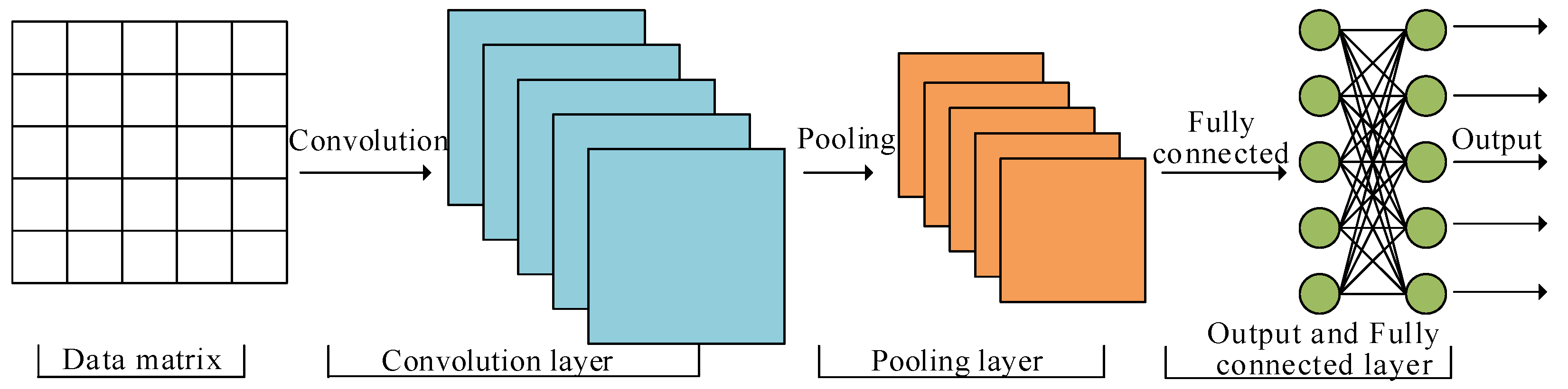
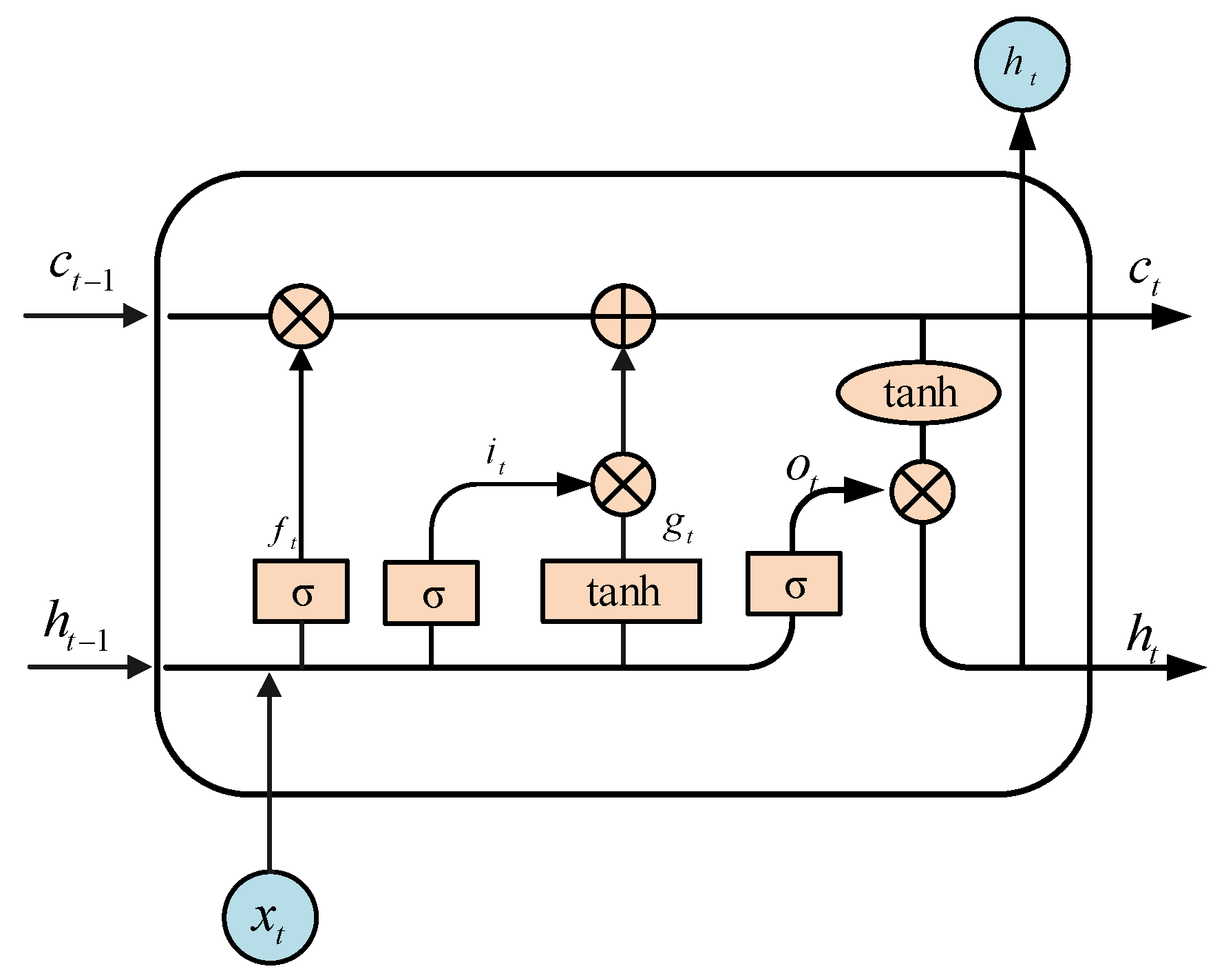
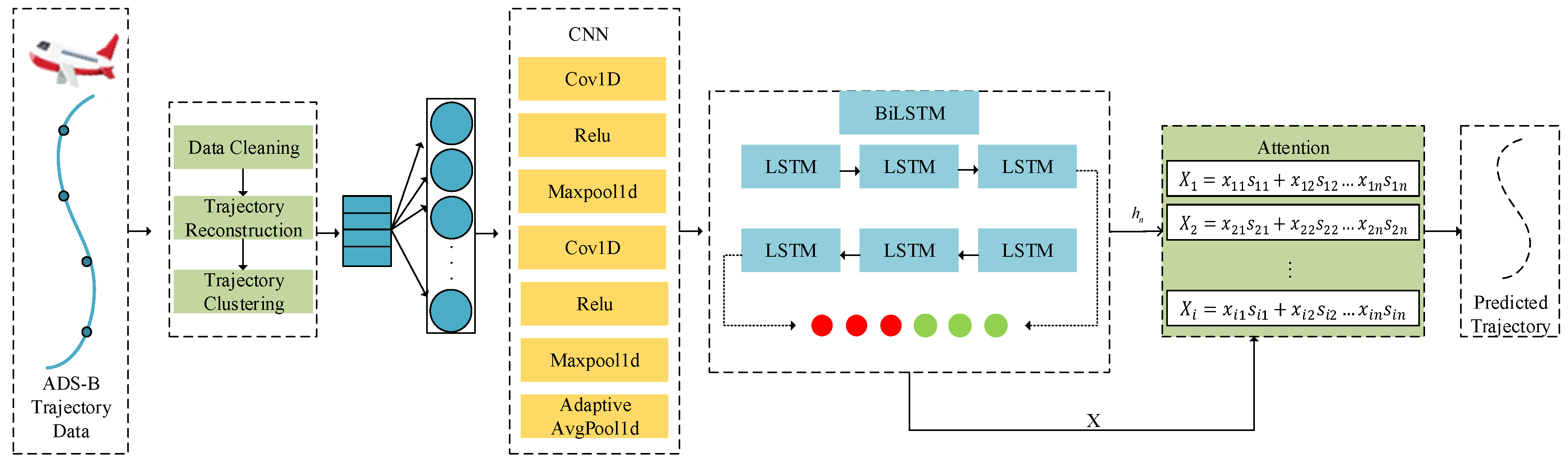
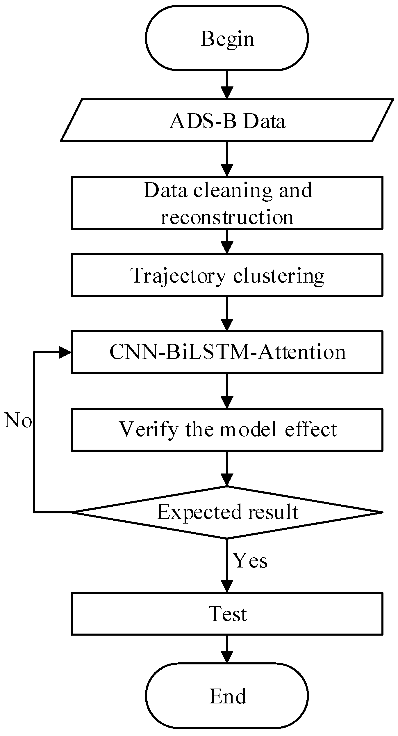
- According to the characteristics of the aircraft trajectory, we designed the CNN–BiLSTM–Attention trajectory prediction model. The CNN model was used to extract the spatial features of each trajectory, the BiLSTM model was used to extract the temporal features, and the attention mechanism was used to learn the weights of different trajectory points;
- (3)
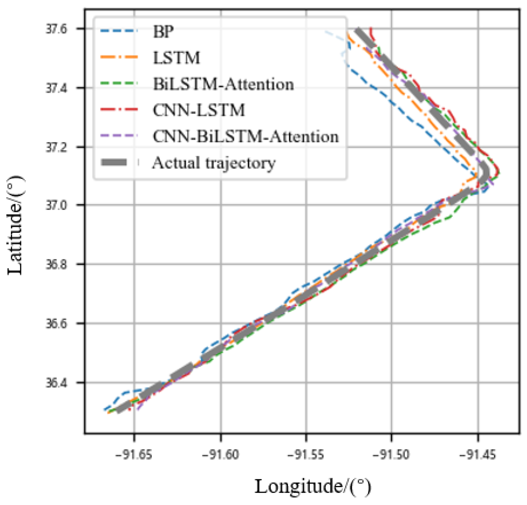
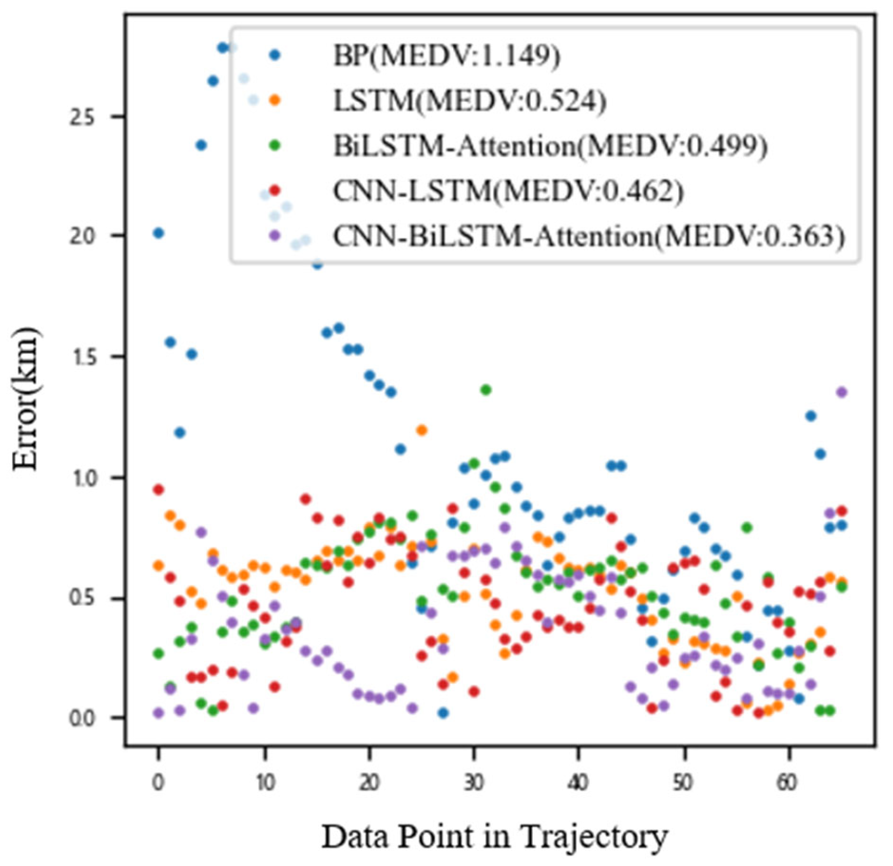
- We compared the constructed model with the BP, LSTM, and CNN–LSTM models and found that the proposed model greatly improved the prediction accuracy, and trajectory clustering can further improve the accuracy.
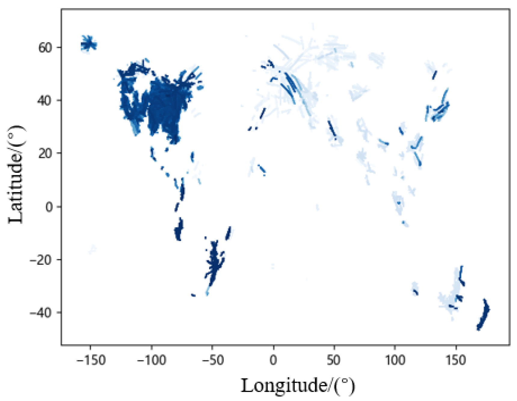
2. Data Preparation
2.1. ADS-B Data
2.2. Feature Selection
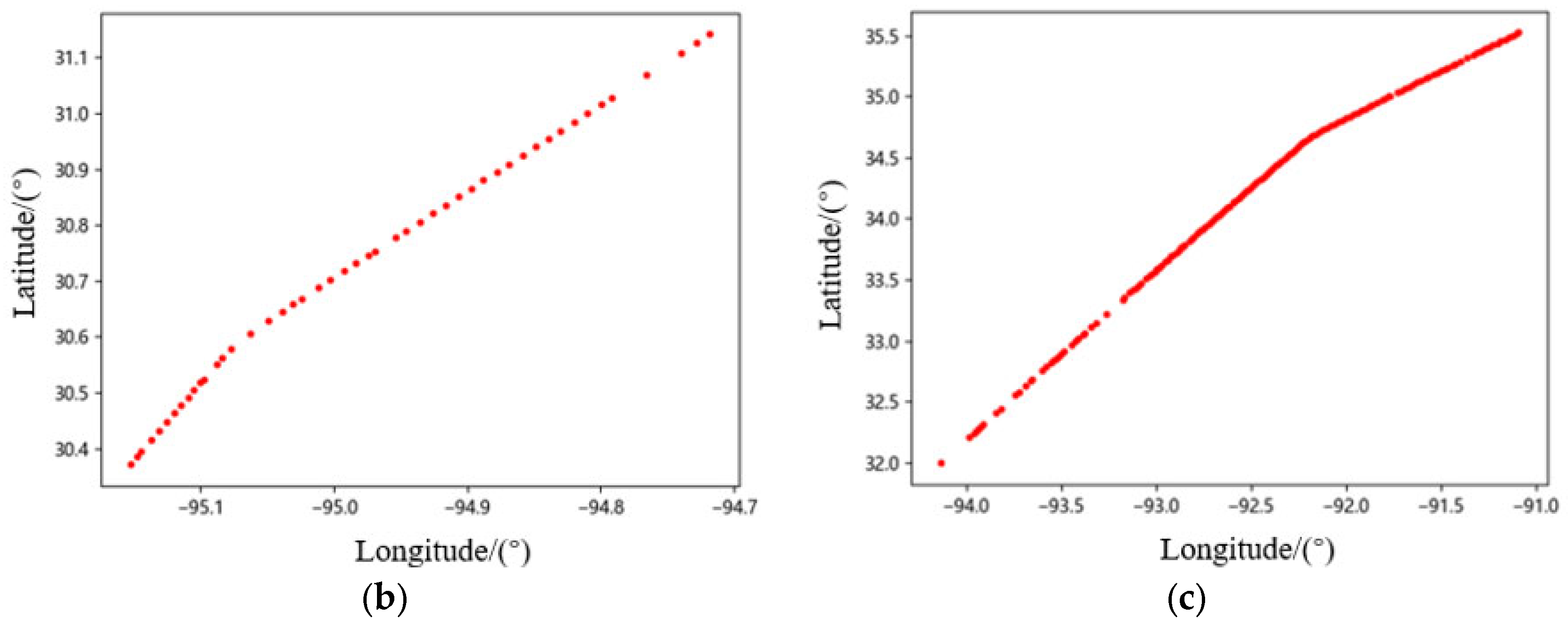
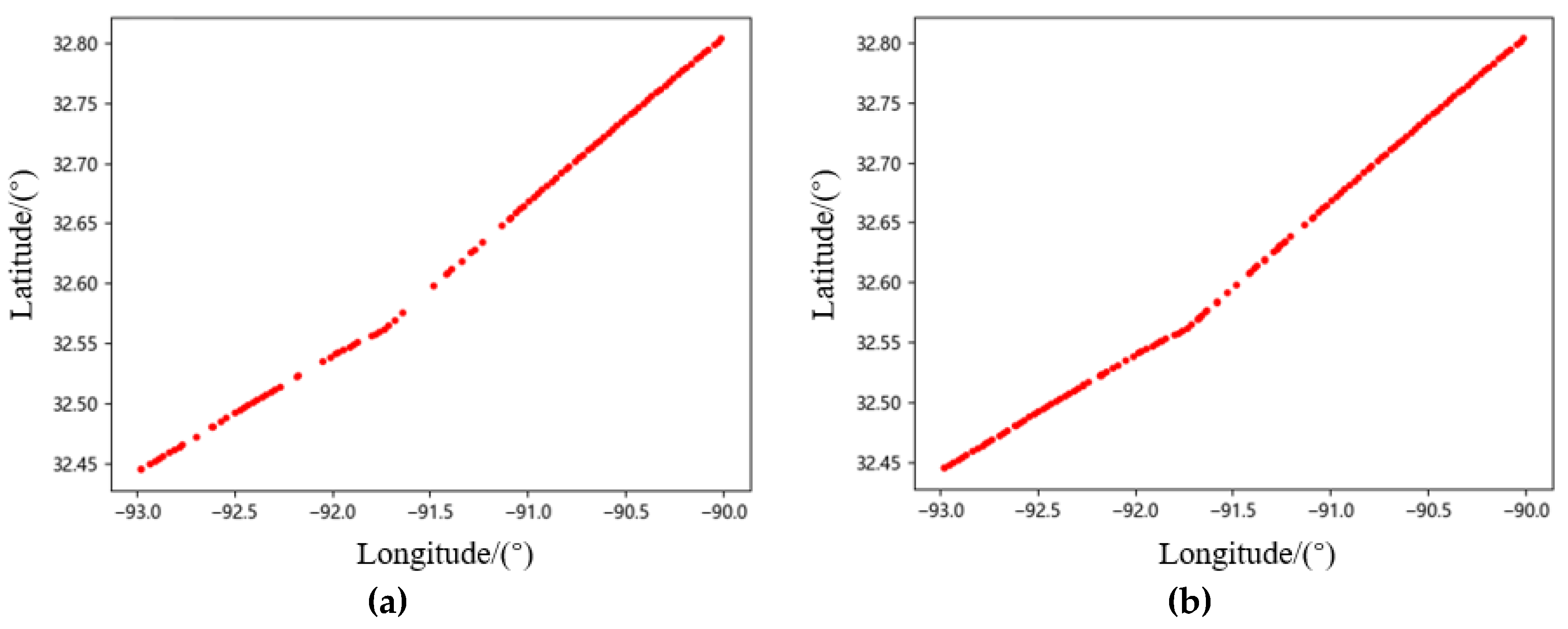
2.3. Cleaning and Reconstruction
2.4. Linear Interpolation
| Algorithm 1: Trajectory Cleaning and Reconstruction |
| Input: ADS-B dataset A |
| Output: Cleaning and Reconstructing Trajectory Dataset F |
| 1: Abnormal data are cleaned and filtered based on region from A; |
| 2: Trajectory C is filtered from A based on the aircraft call sign and stored in dataset D; |
| 3: For C in D: |
| 4: if the number of trajectory points is greater than 30, then |
| 5: if the distance between two adjacent points is more than 30 km, mark it as a breakpoint, then |
| 6: if the number of adjacent breakpoint trajectory points is greater than 30, then |
| 7: save the trajectory in dataset E; |
| 8: else |
| 9: back to step 5 |
| 10: else |
| 11: save the trajectory in dataset E; |
| 12: end |
| 13: else |
| 14: delete the trajectory; |
| 15: end |
| 16: For C in E: |
| 17: if the time between two adjacent points is not continuous, then |
| 18: use linear interpolation to complete the trajectory and save it to dataset F; |
| 19: end. |
3. Trajectory Clustering
3.1. K-Medoids Clustering
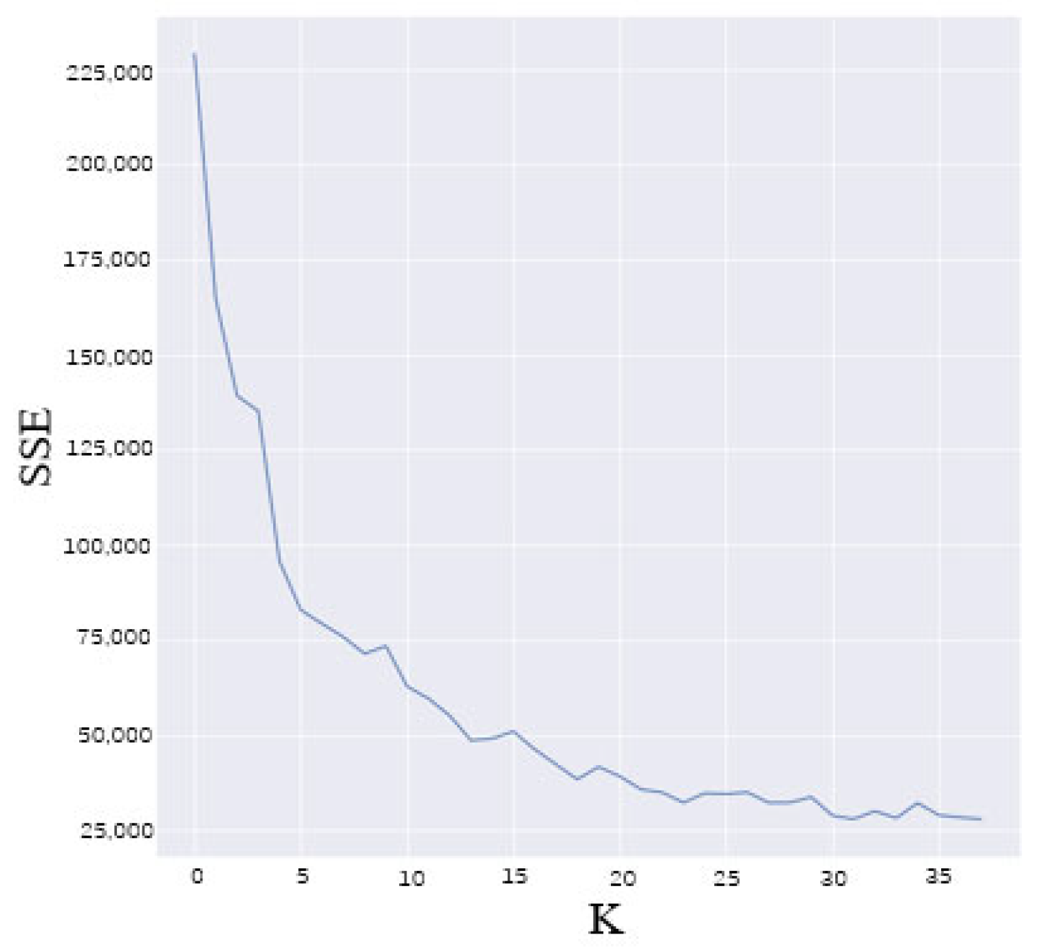
3.2. Number of Clusters
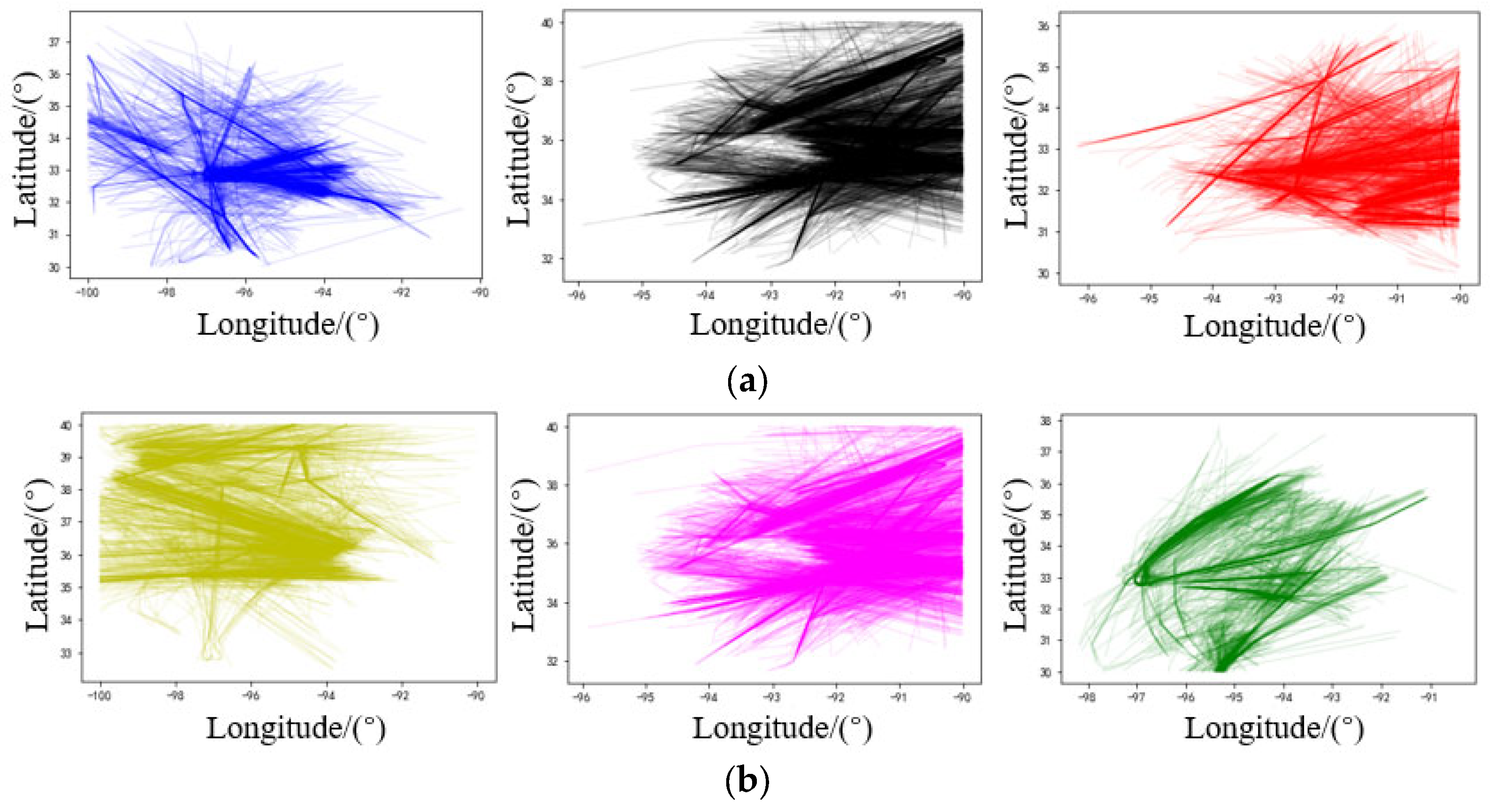
3.3. Clustering Result
4. Trajectory Prediction Model
4.1. CNN
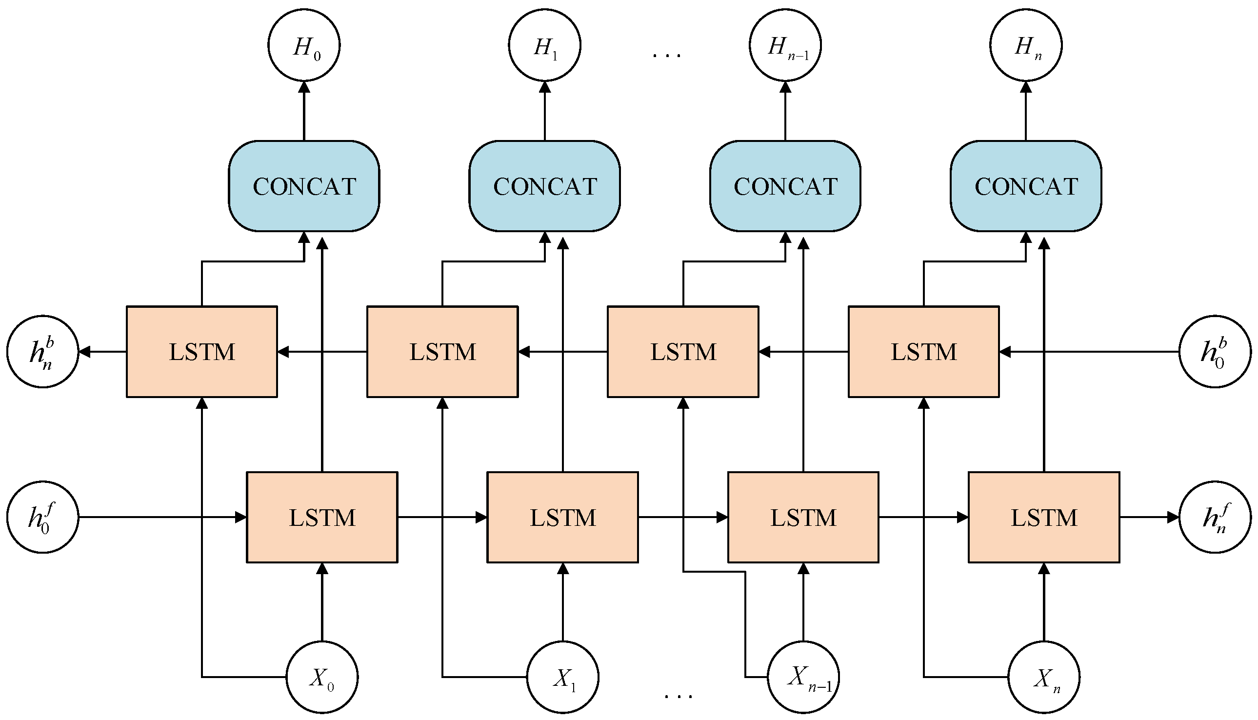
4.2. BiLSTM
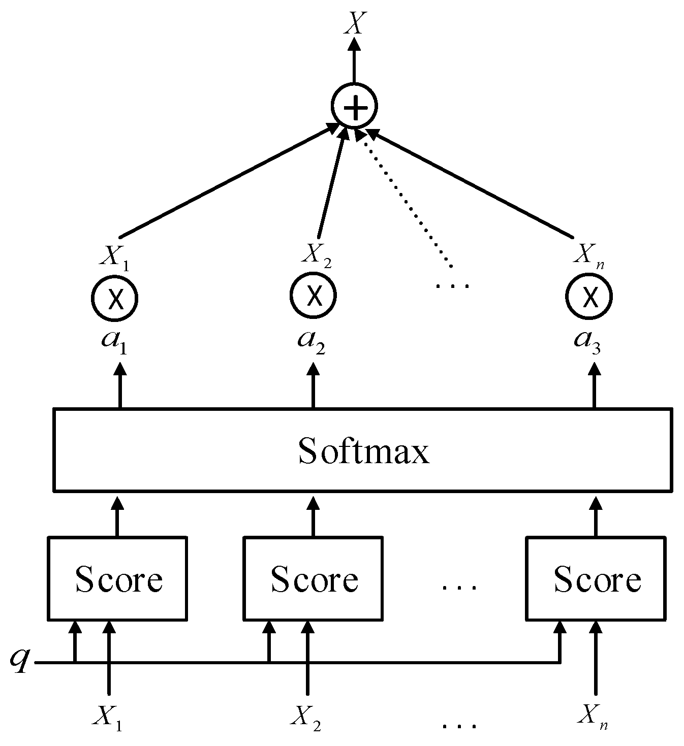
4.3. Attention
4.4. Model Framework
5. Experiment and Analysis
5.1. Experiment Data
5.2. Data Normalization
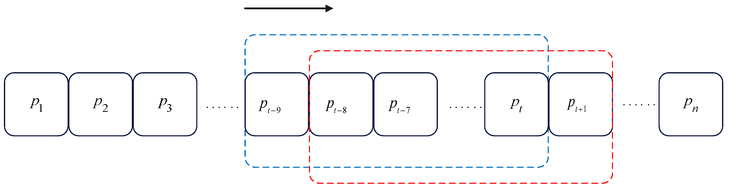
5.3. Sliding Time Window
5.4. Evaluation Indicators
5.5. Comparative Experiment Analysis
6. Conclusions
Author Contributions
Funding
Data Availability Statement
Conflicts of Interest
References
- Cheng, C.; Guo, L.; Wu, T.; Sun, J.; Gui, G.; Adebisi, B.; Gacanin, H.; Sari, H. Machine-Learning-Aided Trajectory Prediction and Conflict Detection for Internet of Aerial Vehicles. IEEE Internet Things J. 2022, 9, 5882–5894. [Google Scholar] [CrossRef]
- Slattery, R.; Zhao, Y. Trajectory Synthesis for Air Traffic Automation. J. Guid. Control. Dyn. 1997, 20, 232–238. [Google Scholar] [CrossRef]
- Harrison, M. ADS-X the Next Gen Approach for the Next Generation Air Transportation System. In Proceedings of the 25th Digital Avionics Systems Conference, Portland, OR, USA, 15–19 October 2006; pp. 1–8. [Google Scholar]
- Luckenbaugh, G.; Landriau, S.; Dehn, J.; Rudolph, S. Service Oriented Architecture for the Next Generation Air Transportation System. In Proceedings of the 2007 Integrated Communications, Navigation and Surveillance Conference, Herndon, VA, USA, 30 April–3 May 2007; pp. 1–9. [Google Scholar]
- Sipe, A.; Moore, J. Air traffic functions in the NextGen and SESAR airspace. In Proceedings of the IEEE/AIAA Digital Avionics Systems Conference, Orlando, FL, USA, 23–29 October 2009; pp. 2.A.6-1–2.A.6-7. [Google Scholar]
- Wang, X.; Jiang, X.; Chen, L.; Wu, Y. KVLMM: A Trajectory Prediction Method Based on a Variable-Order Markov Model With Kernel Smoothing. IEEE Access 2018, 6, 25200–25208. [Google Scholar] [CrossRef]
- Chiou, Y.S.; Wang, C.L.; Yeh, S.C. Reduced-complexity scheme using alpha–beta filtering for location tracking. IET Commun. 2011, 5, 1806–1813. [Google Scholar] [CrossRef]
- Yu, W.; Yu, H.; Du, J.; Zhang, M.; Liu, J. DeepGTT: A general trajectory tracking deep learning algorithm based on dynamic law learning. IET Radar Sonar Navig. 2021, 15, 1125–1150. [Google Scholar] [CrossRef]
- Gao, C.; Yan, J.; Zhou, S.; Varshney, P.K.; Liu, H. Long short-term memory-based deep recurrent neural networks for target tracking. Inf. Sci. 2019, 502, 279–296. [Google Scholar] [CrossRef]
- Kui, Q.; Ying, Z.; Liujing, Y.; Rongping, X.; Xidian, H. Aircraft target track prediction model based on BP neural network. Command. Inf. Syst. Technol. 2017, 8, 54–58. [Google Scholar] [CrossRef]
- Shi, Z.; Xu, M.; Pan, Q.; Yan, B.; Zhang, H. LSTM-based Flight Trajectory Prediction. In Proceedings of the 2018 International Joint Conference on Neural Networks, IJCNN, Rio de Janeiro, Brazil, 8–13 July 2018; pp. 1–8. [Google Scholar]
- Graves, A.; Schmidhuber, J. Framewise phoneme classification with bidirectional LSTM and other neural network architectures. Neural Netw. 2005, 18, 602–610. [Google Scholar] [CrossRef] [PubMed]
- Siami-Namini, S.; Tavakoli, N.; Namin, A.S. The Performance of LSTM and BiLSTM in Forecasting Time Series. In Proceedings of the 2019 IEEE International Conference on Big Data (Big Data), Los Angeles, CA, USA, 9–12 December 2019; pp. 3285–3292. [Google Scholar]
- Xu, Z.; Zeng, W.; Chu, X.; Cao, P. Multi-Aircraft Trajectory Collaborative Prediction Based on Social Long Short-Term Memory Network. Aerospace 2021, 8, 115. [Google Scholar] [CrossRef]
- Ma, L.; Tian, S. A Hybrid CNN-LSTM Model for Aircraft 4D Trajectory Prediction. IEEE Access 2020, 8, 134668–134680. [Google Scholar] [CrossRef]
- Zhou, J.; Zhang, H.; Lyu, W.; Wan, J.; Zhang, J.; Song, W. Hybrid 4-Dimensional Trajectory Prediction Model, Based on the Reconstruction of Prediction Time Span for Aircraft en Route. Sustainability 2022, 14, 3862. [Google Scholar] [CrossRef]
- Zhang, Z.; Gao, J.; Mao, J.; Liu, Y.; Anguelov, D.; Li, C. STINet: Spatio-Temporal-Interactive Network for Pedestrian Detection and Trajectory Prediction. In Proceedings of the 2020 IEEE/CVF Conference on Computer Vision and Pattern Recognition, CVPR, Seattle, WA, USA, 13–19 June 2020; pp. 11343–11352. [Google Scholar]
- Park, J.; Jeong, J.; Park, Y. Ship Trajectory Prediction Based on Bi-LSTM Using Spectral-Clustered AIS Data. J. Mar. Sci. Eng. 2021, 9, 1037. [Google Scholar] [CrossRef]
- Sun, J.; Ellerbroek, J.; Hoekstra, J. Flight Extraction and Phase Identification for Large Automatic Dependent Surveillance–Broadcast Datasets. J. Aerosp. Inf. Syst. 2017, 14, 566–572. [Google Scholar] [CrossRef] [Green Version]
- Vaughan, N.; Gabrys, B. Comparing and Combining Time Series Trajectories Using Dynamic Time Warping. Procedia Comput. Sci. 2016, 96, 465–474. [Google Scholar] [CrossRef] [Green Version]
- Chen, Z.; Yan, Y.; Ellis, T. Lane detection by trajectory clustering in urban environments. In Proceedings of the IEEE International Conference on Intelligent Transportation Systems, Qingdao, China, 8–11 October 2014; pp. 3076–3081. [Google Scholar]
- Bergroth, L.; Hakonen, H.; Raita, T. A survey of longest common subsequence algorithms. In Proceedings of the International Symposium on String Processing & Information Retrieval, A Curuna, Spain, 27–29 September 2000; pp. 39–48. [Google Scholar]
- Laxhammar, R.; Falkman, G. Online Learning and Sequential Anomaly Detection in Trajectories. IEEE Trans. Pattern Anal. Mach. Intell. 2014, 36, 1158–1173. [Google Scholar] [CrossRef] [PubMed]
- Arora, P.; Deepali; Varshney, S. Analysis of K-Means and K-Medoids Algorithm for Big Data. Procedia Comput. Sci. 2016, 78, 507–512. [Google Scholar] [CrossRef] [Green Version]
- Aranganayagi, S.; Thangavel, K. Clustering Categorical Data Using Silhouette Coefficient as a Relocating Measure. In Proceedings of the International Conference on Computational Intelligence and Multimedia Applications, ICCIMA 2007, Sivakasi, India, 13–15 December 2007; pp. 13–17. [Google Scholar]
- Liu, L.; Zhai, L.; Han, Y. Aircraft trajectory prediction based on convLSTM. Comput. Eng. Des. 2022, 43, 1127–1133. [Google Scholar] [CrossRef]
- Mnih, V.; Heess, N.; Graves, A.; Kavukcuoglu, K. Recurrent Models of Visual Attention. Adv. Neural Inf. Process. Syst. 2014, 3. [Google Scholar] [CrossRef]
- Zhang, S.; Wang, L.; Zhu, M.; Chen, S.; Zhang, H.; Zeng, Z. A Bi-directional LSTM Ship Trajectory Prediction Method based on Attention Mechanism. In Proceedings of the 2021 IEEE 5th Advanced Information Technology, Electronic and Automation Control Conference, IAEAC, Chongqing, China, 12–14 March 2021; pp. 1987–1993. [Google Scholar]


| Name | Meaning | Example |
|---|---|---|
| Latitude | The latitude of the aircraft | 35.05178833 |
| Longitude | The longitude of the aircraft | −90.35195487 |
| Velocity | The speed over the ground of the aircraft | 144.7865144 |
| Heading | The direction of movement as the clockwise angle from the geographic north | 288.4349488 |
| Category 1 | Category 2 | Category 3 | Category 4 | Category 5 | Category 6 |
|---|---|---|---|---|---|
| 3641 | 2903 | 3400 | 3639 | 5868 | 3323 |
| Model | Evaluation Indicators | ||||||
|---|---|---|---|---|---|---|---|
| Latitude | Longitude | MEDV/km | |||||
| MAE | RMSE | MAPE/% | MAE | RMSE | MAPE/% | ||
| BP | 0.0215 | 0.0245 | 0.0614 | 0.0139 | 0.0176 | 0.0151 | 1.562 |
| LSTM | 0.0096 | 0.0115 | 0.0271 | 0.0095 | 0.0121 | 0.0105 | 1.069 |
| BiLSTM–Attention | 0.0086 | 0.0109 | 0.0243 | 0.0084 | 0.0114 | 0.0915 | 0.939 |
| CNN–LSTM | 0.0077 | 0.0099 | 0.0218 | 0.0081 | 0.0114 | 0.0088 | 0.906 |
| CNN–BiLSTM–Attention | 0.0068 | 0.0090 | 0.0192 | 0.0075 | 0.0106 | 0.0081 | 0.838 |
| Model | Dataset | Evaluation Indicators | ||||||
|---|---|---|---|---|---|---|---|---|
| Latitude | Longitude | MEDV/km | ||||||
| MAE | RMSE | MAPE/% | MAE | RMSE | MAPE/% | |||
| CNN–BiLSTM–Attention | 0.0158 | 0.0183 | 0.0443 | 0.0187 | 0.0223 | 0.0203 | 2.088 | |
| 0.0068 | 0.0090 | 0.0192 | 0.0075 | 0.0106 | 0.0081 | 0.838 | ||
Publisher’s Note: MDPI stays neutral with regard to jurisdictional claims in published maps and institutional affiliations. |
© 2022 by the authors. Licensee MDPI, Basel, Switzerland. This article is an open access article distributed under the terms and conditions of the Creative Commons Attribution (CC BY) license (https://creativecommons.org/licenses/by/4.0/).
Share and Cite
Wu, Y.; Yu, H.; Du, J.; Liu, B.; Yu, W. An Aircraft Trajectory Prediction Method Based on Trajectory Clustering and a Spatiotemporal Feature Network. Electronics 2022, 11, 3453. https://doi.org/10.3390/electronics11213453
Wu Y, Yu H, Du J, Liu B, Yu W. An Aircraft Trajectory Prediction Method Based on Trajectory Clustering and a Spatiotemporal Feature Network. Electronics. 2022; 11(21):3453. https://doi.org/10.3390/electronics11213453
Chicago/Turabian StyleWu, You, Hongyi Yu, Jianping Du, Bo Liu, and Wanting Yu. 2022. "An Aircraft Trajectory Prediction Method Based on Trajectory Clustering and a Spatiotemporal Feature Network" Electronics 11, no. 21: 3453. https://doi.org/10.3390/electronics11213453