Article

Collaborative Accurate Vehicle Positioning Based on Global Navigation Satellite System and Vehicle Network Communication

1
State Key Laboratory of Automotive Simulation and Control, Jilin University, Changchun 130025, China
2
School of Mechanical Engineering, University of Science and Technology Beijing, Beijing 100083, China
3
Shunde Innovation School, University of Science and Technology Beijing, Foshan 528399, China
4
Department of Waterway Transport and Maritime Management, Beijing Vocational College of Transportation, Beijing 102600, China
*
Authors to whom correspondence should be addressed.
Electronics 2022, 11(19), 3247; https://doi.org/10.3390/electronics11193247
Submission received: 14 September 2022 / Revised: 4 October 2022 / Accepted: 7 October 2022 / Published: 9 October 2022

Abstract

:
Intelligence is a direction of development for vehicles and transportation. Accurate vehicle positioning plays a vital role in intelligent driving and transportation. In the case of obstruction or too few satellites, the positioning capability of the Global navigation satellite system (GNSS) will be significantly reduced. To eliminate the effect of unlocalization due to missing GNSS signals, a collaborative multi-vehicle localization scheme based on GNSS and vehicle networks is proposed. The vehicle first estimates the location based on GNSS positioning information and then shares this information with the environmental vehicles through vehicle network communication. The vehicle further integrates the relative position of the ambient vehicle observed by the radar with the ambient vehicle position information obtained by communication. A smaller error estimate of the position of self-vehicle and environmental vehicles is obtained by correcting the positioning of self-vehicle and environmental vehicles. The proposed method is validated by simulating multi-vehicle motion scenarios in both lane change and straight-ahead scenarios. The root-mean-square error of the co-location method is below 0.5 m. The results demonstrate that the combined vehicle network communication approach has higher accuracy than single GNSS positioning in both scenarios.

1. Introduction

In recent years, the degree of automation of intelligent vehicles has gradually increased [1,2]. Intelligent vehicles can primarily reduce the influence of human factors and decrease the occurrence of traffic accidents [3]. Highly accurate positioning is the basis for intelligent vehicles to achieve path planning and motion trajectory tracking. In the development of in-vehicle navigation, driver assistance, autonomous driving, intelligent transportation and other technologies [4], the location of the vehicle is a critical type of information. GNSS is currently an essential method in vehicle positioning [5,6]. However, the positioning can be inaccurate or even impossible if there are tunnels and other occlusions. This single positioning method cannot fully meet the needs of the growing automotive intelligence in terms of accuracy and reliability. Therefore, it is important to explore new vehicle localization methods to develop intelligent driving and intelligent transportation.
Researchers made many efforts in vehicle positioning, which contains methods of multi-sensor fusion, vehicle network communication and artificial intelligence. In fusing information from multiple sensors, Pankaj et al. [7] proposed an optical camera-based mobile vehicle localization scheme. Using the street light and camera as transmitter and receiver, respectively, it is able to achieve a positioning accuracy of less than 1 m. Ioannis et al. [8] used distance and velocity measurements to deal with localization and target tracking problems. This approach enabled localization despite the absence of GNSS signals. Patrick et al. [9] performed position estimation by installing fixed points on the road and detecting body bumps and road surface imperfections. Hossain et al. [10] matched and fused the position information obtained from GNSS, vehicle network communication and radar. The simulation results showed a significant improvement in positioning accuracy. Wang et al. [11] proposed an auxiliary vehicle location system. The system consists of three base stations equipped with multiple inputs and multiple outputs. Accurate localization can be achieved based on the results of three cross-locations. Tao et al. [12] proposed a multi-sensor fusion localization strategy for intelligent vehicles using global pose map optimization and validated it on the ROS platform. Zhang et al. [13,14] proposed a collaborative positioning method based on 3D mapping-assisted GNSS. The technique utilized measurements from surrounding available GNSS receivers, eliminating systematic errors while also mitigating random errors. The multi-sensor fusion approach makes the vehicle more costly, and the sensors are more affected by the environment.
If only the vehicles are individually positioned by sensors, autonomous vehicle positioning may not be possible in the absence of signals. The development of Telematics technology allows the use of location data from nearby vehicles to improve or replace self-location. Nam et al. [15] proposed a cooperative adjacent vehicle localization system. The system quickly identifies the location of neighboring vehicles and communicates that information with neighboring vehicles. Zhu et al. [16] established a GNSS/dead reckoning/ultra-wide band fusion positioning algorithm with adaptive information allocation coefficients using the Kalman filter, which can improve positioning accuracy and reliability. Mahmoud et al. [17] used dedicated short-range communications to share data between vehicles, enabling the positioning of vehicles during GNSS signal outages. Hou et al. [18] proposed a displacement-based selection method that can reduce the effect of measurement errors in nearby vehicle information. The status information of nearby vehicles can be used to locate the target vehicle. Buehrer et al. [19] considered the application of IoT and 5G to co-location, demonstrating its superior coverage and accuracy. Ma et al. [20] proposed a BeiDou-based joint vehicle-road positioning method using the volumetric Kalman model to further improve the positioning accuracy. Ansari et al. [21] investigated the supplementation of dedicated short-range communication and V2V by terrestrial communication systems to examine the positioning performance of vehicles. Tong et al. [22] used information collection platforms to obtain driving status and roadside information to obtain the vehicle’s location. The current method still has room for improvement in the integration of GNSS, vehicle network communication, and vehicle sensors. Positioning accuracy still needs to be improved.
With the advancement of computer technology, artificial intelligence methods are increasingly used in vehicle positioning. Kim et al. [23] developed an indoor vehicle location system using surveillance cameras. Such a system determines the location of a vehicle by extracting vehicle information from image information. Wan et al. [24] combined machine learning and edge computing and could obtain high accuracy in vehicle location estimation. Lee et al. [25] developed a machine learning method applicable to location prediction using the data generated by the localization algorithm, which improved the accuracy of location prediction by 10%. Kong et al. [26] proposed a vehicle localization system based on federated learning. The system makes full use of edge computing and can provide high-accuracy positioning correction. Gao et al. [27] proposed an error-weighting-based vehicle localization fusion algorithm. Distance and positioning compound errors are taken into account for single-vehicle positioning and trilateral positioning. Wang et al. [28] studied the effects of vehicle location potential features and vehicle association potential features. A routing algorithm based on vehicle location analysis is proposed to obtain more accurate vehicle location prediction. Watta et al. [29] proposed an intelligent system incorporating neural networks and geometric modeling. A neural network trained on V2V signals to obtain the location of remote vehicles. Figure 1 shows the different methods of vehicle positioning. Machine learning methods are considered to be black-box models. There is no way to know the direction of learning inside the model, and the application of such methods is still open to question. The collaborative localization method proposed in this study combines GNSS, vehicle network communication and in-vehicle sensors to achieve more accurate vehicle positioning.
A collaborative vehicle positioning method using GNSS and vehicle network communication is proposed in order to overcome the shortcomings of GNSS positioning in terms of accuracy and reliability. Contributions of this paper are shown in the following aspects:
(1) GNSS and vehicle network communication: Combined positioning using GNSS and vehicle network communication to improve positioning accuracy and reliability.
(2) Multi-vehicle scenario validation: A multi-vehicle motion scenario was built, and the positioning was verified under straight-ahead and lane change conditions.
(3) Impact of communication interruption: Verification of positioning accuracy during communication interruption to check the effectiveness of vehicle network communication for positioning.
The remainder of this paper is structured as follows: Section 2 describes the vehicle model and the multi-vehicle motion scenario used for simulation. Section 3 compares the positioning accuracy in different positioning scenarios, and Section 4 gives the conclusion of the study.

2. Research Methodology

The proposed methodology uses GNSS and vehicle network communication. To verify the method’s effectiveness, kinematic modeling of the vehicle is performed. A motion scene is created in the simulation environment and the positioning error is calculated.

2.1. Component Modules
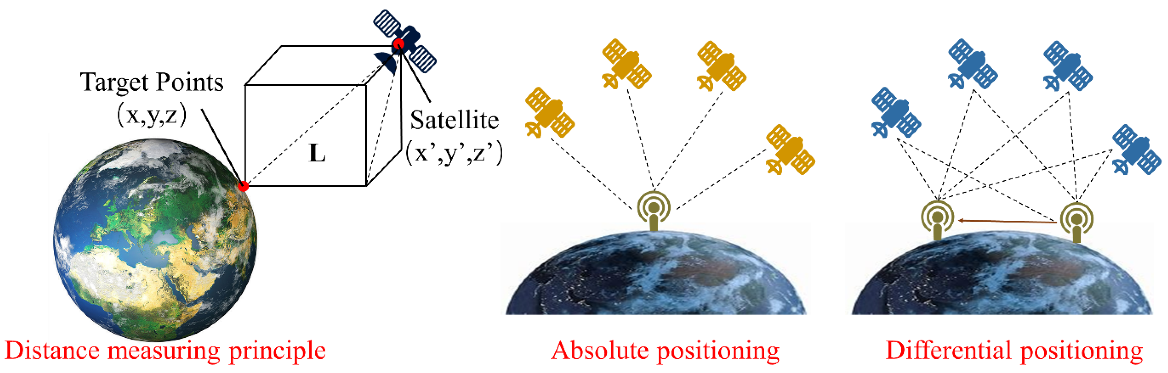
The proposed multi-vehicle cooperative positioning system consists of three modules: GNSS, millimeter wave radar and vehicle network communication.

2.1.1. GNSS

GNSS is a navigation and positioning system that uses radio. It refers to all satellite navigation systems, such as GPS of the United States, Glonass of Russia, Galileo of Europe and BeiDou of China. It can provide 3D coordinates, velocity and time information at any of Earth’s surfaces or near-Earth space. These three types of information are called PVT (Position Velocity and Time). In this study, absolute position information of the vehicle can be obtained using GNSS. The received coordinates are earth latitude and longitude coordinates, which can be converted to local area plane coordinates by calculation.
As shown in Figure 2, any location on the Earth’s surface has a three-dimensional coordinate. GNSS satellites also have a coordinate. The distance between the satellite and the positioning target can be expressed in coordinates as
L = ( x x ) 2 + ( y y ) 2 + ( z z ) 2
where the coordinates of the satellite are known and the target point coordinates are unknown.
The speed of signal transmission between the satellite and the target point can be regarded as the light speed. Then the distance between the satellite and the target point can be expressed as
L = ( t t ) · c
where t is the satellite time and t is the time at the target point. Combining the two equations, we get
( t t ) · c = ( x x ) 2 + ( y y ) 2 + ( z z ) 2
At this point, the coordinate values of the other three satellites are needed to solve the equation. It takes at least four satellites to determine the location of a target point on Earth. Depending on the number of signal receivers, positioning can also be divided into absolute positioning and differential positioning.

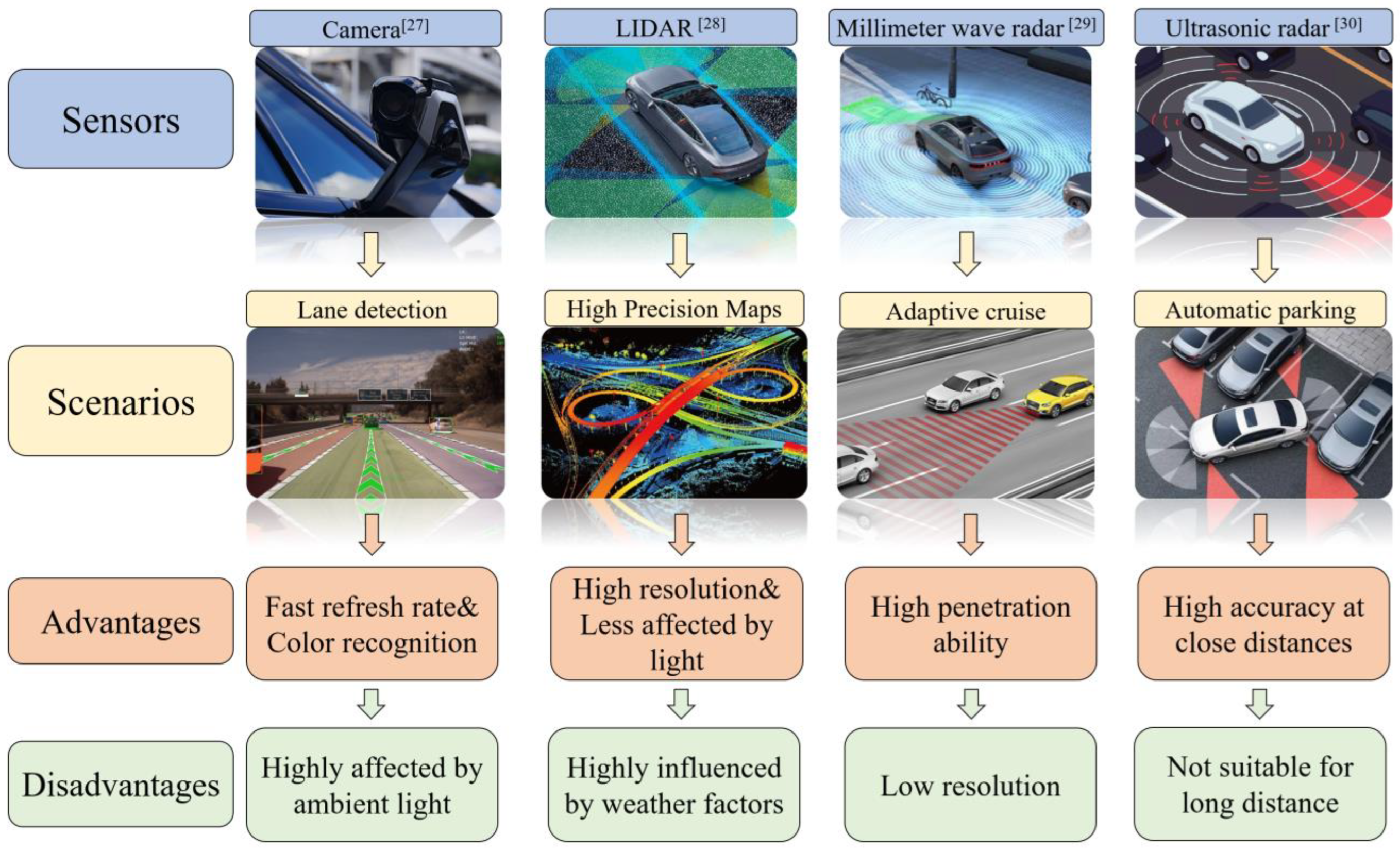
2.1.2. Millimeter Wave Radar

The use of millimeter wave radar can obtain the relative position information of nearby environmental vehicles to the present vehicle. This includes the distance and angle of the ambient vehicle relative to the vehicle, that is, the position of the ambient vehicle in the local coordinate system.
Sensors commonly used for environmental awareness in smart vehicles include cameras, Light Detection and Ranging (LIDAR), millimeter-wave radar and ultrasonic radar. The camera is a component based on the optical principle [30]. When the light passes through the lens, it is captured by the light sensor and then forms an image. LIDAR performs object detection and ranging by emitting laser pulses externally [31]. The laser will reflect when it reaches the surface of the target to be measured. LIDAR can acquire parameters such as the reflected signal’s return time and signal strength. The information allows us to determine the target’s distance, orientation, motion status and other characteristics. Millimeter wave radar is similar to LIDAR in principle. The difference is that the signal it emits is changed from laser to electromagnetic wave [32]. It calculates the distance from the time difference of electromagnetic wave returns and calculates the relative velocity of the measured target based on the Doppler effect. The principle of ultrasonic radar is also similar. The signal it generates is ultrasonic [33]. Due to the different principles of the above sensors, the application scenarios are different. Figure 3 illustrates the characteristics of several sensors and their application scenarios.

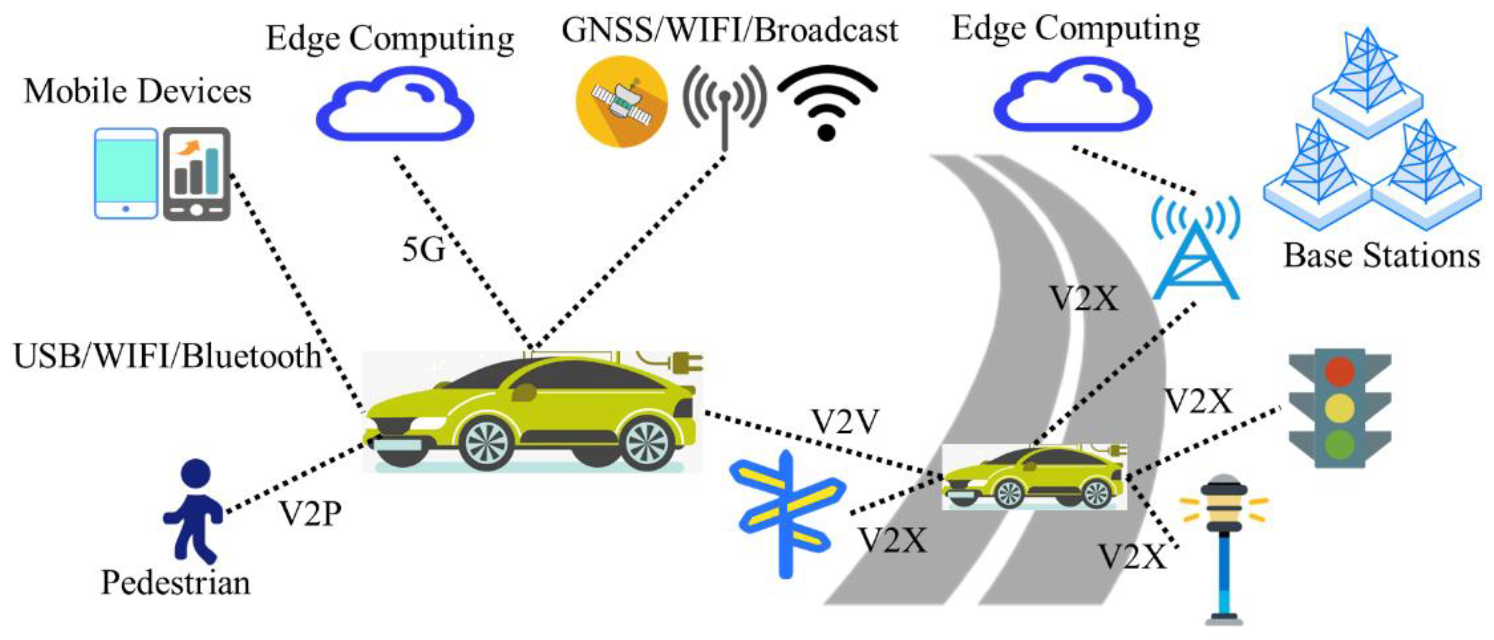
2.1.3. Vehicle Network Communication

Vehicle network refers to a system network for wireless communication and information exchange among vehicles, roads, pedestrians and the Internet based on intra-vehicle network, inter-vehicle network and in-vehicle mobile Internet, in accordance with agreed communication protocols and data interaction standards. Vehicle network is an intelligent three-dimensional architecture, including the data sensing layer, network transmission layer and platform application layer. The data sensing layer uses sensors to perceive information and obtain comprehensive information on road conditions. The network transmission layer connects the infrastructure to the platform application layer. It enables the transfer of information between various subjects. The platform application layer has the function of management and operation. It is capable of performing tasks such as traffic management and safety control.
The main units in the vehicle network communication are shown in Figure 4. Vehicle network communication can be based on dedicated short-range communication (DSRC) or 5G networks to enable the transfer of information between vehicles. This also represents the two main technical routes of the current vehicle network communication standards, namely DSRC and cellular vehicle to everything (C-V2X). DSRC has the technical characteristics of exclusive bandwidth and short-range communication. C-V2X highlights the advantages in capacity, latency, manageability and anti-interference algorithms. In collaborative positioning, when the GNSS signal is missing, the vehicle with the missing signal can establish communication with other vehicles with a normal signal through the vehicle network. Thus, the position of the signal-less vehicle can be determined by the position of the surrounding vehicles with normal signals.

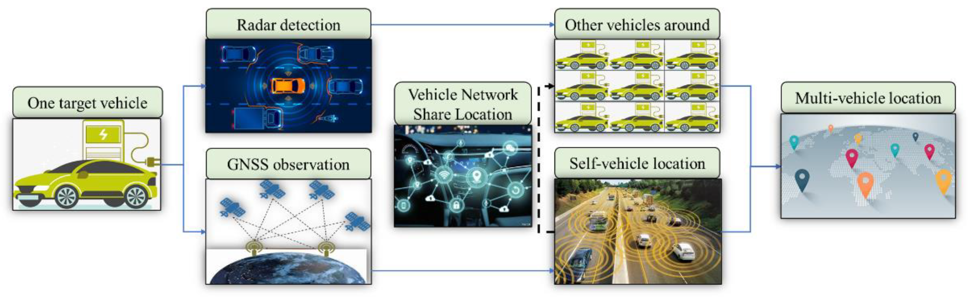
2.2. Overall Flow of the Method

The overall workflow of multi-vehicle cooperative positioning is shown in Figure 5.
The GNSS module obtains absolute vehicle position information with noise [34]. By designing filters to process the signals, coarse position estimation based on self-vehicle observation information can be achieved. Vehicle network communication sends this coarse estimate of position to other vehicles in the vicinity. Combined with the relative position information detected by millimeter wave radar, multi-vehicle cooperative localization is enabled.
Four vehicles (A, B, C and D) are connected by a vehicle network. Each vehicle can position itself via GNSS. Vehicles can communicate with each other via vehicle networks to share location information with other vehicles. The vehicle can sense the relative position within a certain distance by millimeter wave radar. Combined with the information, the vehicle can estimate its own position as well as the position of other vehicles around it. The interrelationship between the vehicles is shown in Figure 6a.

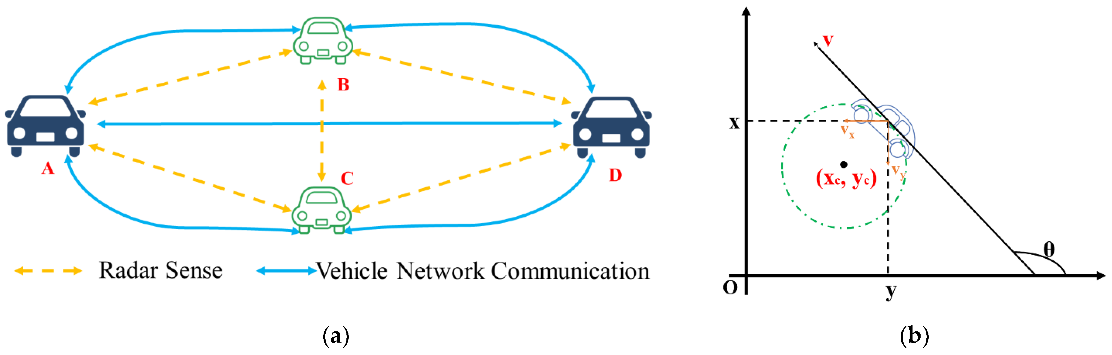
2.3. Vehicle Modeling Based on Velocity Motion Model

The velocity motion model contains linear and angular velocities [35]. The control vector for vehicle motion is:
u t = ( v t w t )
where v t represents the linear velocity of the vehicle and w t represents the angular velocity at the moment t . When v t is positive, the vehicle moves forward. When w t is positive, the vehicle turns counterclockwise.
The state vector of the velocity motion model is:
x t = ( x t y t θ t )
where x t and y t are the position coordinates in the right-angle coordinate system [36], θ t is the velocity direction. The motion of the vehicle is shown in Figure 6b.
Noise can interfere with signal transmission and cause deviations in the state vector and control vector. The location information obtained will be inaccurate. In the ideal case (no noise influence), assume that the initial state vector is ( x ,   y , θ ) T , the control vector is ( v , w ) T and the state vector after Δ t time is ( x , y , θ ) T . The state vector can be expressed as
( x y θ ) = ( x c + v ω sin ( θ + ω Δ t ) y c v ω cos ( θ + ω Δ t ) θ + ω Δ t ) = ( x y θ ) + ( v ω sin θ + v ω sin ( θ + ω Δ t ) v ω cos θ v ω cos ( θ + ω Δ t ) ω Δ t )
where x c = x v ω sin θ , y c = y + v ω cos θ . ( x c ,   y c ) T is the center of the circle for the motion in time Δ t . Considering the error between the real motion and ideal motion of the vehicle and the effect of noise, the real motion model of the vehicle can be expressed as
( x y θ ) = ( x y θ ) + ( v ˇ ω ˇ sin θ + v ˇ ω ˇ sin ( θ + ω ˇ Δ t ) v ˇ ω ˇ cos θ v ˇ ω ˇ cos ( θ + ω ˇ Δ t ) ω ˇ Δ t + γ ˇ Δ t )
v ˇ , ω ˇ should be the filtered value.

2.4. Estimation of Vehicle Location by Relative Positioning

When there are multiple vehicles in the environment for cooperative localization, one of the vehicles is selected as the target vehicle for ease of study and accuracy in presentation. The GNSS signal is filtered to obtain the position estimation result of this vehicle [37]. The results are sent to nearby vehicles via the vehicle network. At the same time, the vehicle can detect the position of nearby environmental vehicles relative to the vehicle through millimeter wave radar. Through the correspondence between the radar target and the ambient vehicle, the position of the ambient vehicle can be used to solve for the position of this vehicle.
The position of this vehicle is obtained from the position and relative distance of the environment vehicle as
μ r t i = ( μ t , x i d t i cos φ t i ,   μ t , y i d t i sin φ t i ) T
where μ t , x i and μ t , y i are the coordinates of the environment vehicle and d t i is the distance between this vehicle and the ambient vehicle. Assume that the error of the radar measurement at the moment t is
ε t , r = ( ε t , rx , ε t , ry ) T
The two follow a normal distribution and are uncorrelated with each other. Then there are
ε t , rx ~ N ( 0 , σ rx 2 ) ,   ε t , ry ~ N ( 0 , σ ry 2 )
The covariance matrix of the radar range can be obtained as
P = ( σ rx 2 0 0 σ ry 2 )

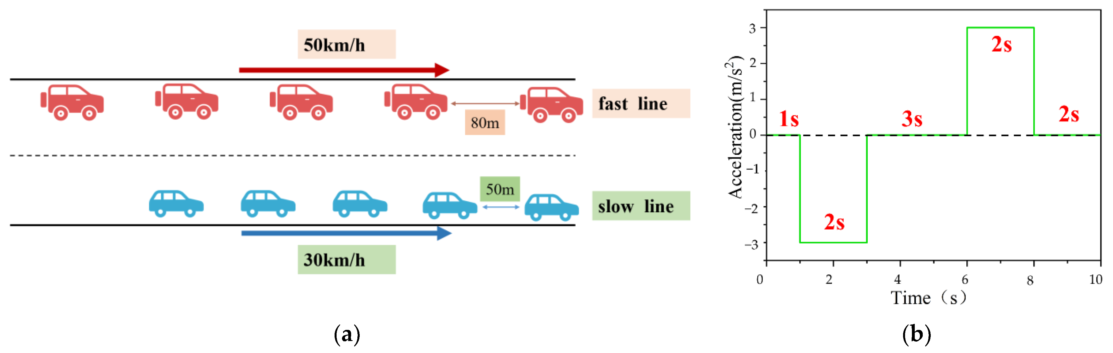
2.5. Simulation Contents

To verify the effectiveness of the method, the simulation is performed by building a multi-vehicle motion scenario. The time duration of each simulation is set to 30 s, and the step size is 0.1 s.

2.5.1. Linear Motion Simulation

The motion scenario contains two lanes. The width of the lanes is 3.75 m, and there are five vehicles in each lane. Vehicles travel along the centerline of their respective lanes. Vehicles located in the fast lane have an initial speed of 50 km/h and a vehicle spacing of 80 m. Vehicles located in the slow lane have an initial speed of 30 km/h and a vehicle spacing of 50 m, as shown in Figure 7a. After the simulation starts, at 0 < t < 10 s, the first car in both lanes moves according to the acceleration curve shown in Figure 7b. At t > 10 s, the first car in both lanes maintains uniform linear motion.
The eight cars after the first car respond to the speed fluctuations of the preceding car according to the linear-following model.
x ¨ r ( t + T ) = λ ( x ˙ f ( t ) x ˙ r ( t ) )
where x ˙ r ( t ) and x ˙ f ( t ) are the distance between the rear car and the front car along the direction of the lane to the origin at time t . Take λ = 0.3 ,   T = 1   s . The motion simulation takes into account the fluctuation of vehicle speed under linear motion and the change of surrounding environment vehicles with time.

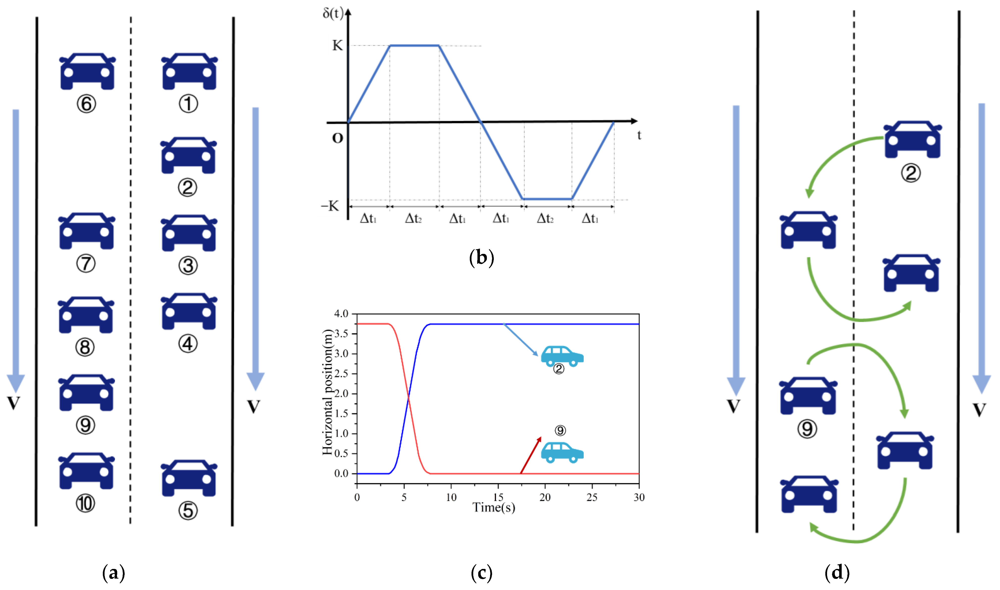
2.5.2. Lane Change Motion Simulation

The motion scenario contains two lanes. The width of the lanes is 3.75 m, and there are five vehicles in each lane. Vehicles travel along the centerline of their respective lanes. The initial speed of both lanes is 30 km/h, and the distance between cars No.4 and No.5 and between cars No.6 and No.7 is 100 m. The distance between the front and rear of other vehicles is 50 m, as shown in Figure 8a.
After starting the simulation, cars 2 and 9 perform the lane change operation at 3 s < t < 8 s, while the other vehicles maintain uniform linear motion. The lane change steering angle is shown in Figure 8b. δ ( t ) is the steering angle at time t . Assuming a linear two-degree-of-freedom model for the vehicle, with constant longitudinal velocity and small angular offset in the heading. Then δ ( t ) function satisfies that the transverse pendulum angular velocity, lateral velocity and heading angular deflection are zero at the beginning and end of steering. Simplifying the velocity motion model assumes a zero lateral deflection angle. Therefore, the angular velocity of the vehicle transverse pendulum is proportional to the steering angle, and δ ( t ) can be replaced by ω ( t ) .
To determine the parameters K ,   Δ t 1 ,   Δ t 2 in this channel change model, the constraints are listed. The lateral displacement, maximum lateral acceleration and maximum lateral sharpness are constrained, respectively
y l u = lim t 0 t 0 τ ω ( α ) d α   d t
| a l a t e r a l ( t ) | < 0.2   g
| a ˙ l a t e r a l ( t ) | < 0.1   g s
where y l is the target lateral displacement, u is the vehicle longitudinal velocity, v is the lateral velocity of the vehicle, g is the acceleration of gravity and a l a t e r a l is the lateral acceleration
a l a t e r a l = v ˙ u ω u ω
Substituting into the channel change model, we get
K ( 2 Δ t 1 2 + 3   Δ t 1 Δ t 2 + Δ t 2 2 ) = y l u
K u < 0.2   g
K u Δ t 1 < 0.1   g s
where y l = 3.75   m ,   u = 30   km / h , The value of the parameter satisfying the above constraint is solved as K = 0.12   rad / s , Δ t 1 = 1   s , Δ t 2 = 0.5   s . The corresponding lane change curve is shown in Figure 8c. Figure 8d displays Car 2 and Car 9 for lane change simulation.
At 9 s < t < 19 s, the first car in both lanes moves in the same way as Figure 7b: “uniform speed—uniform deceleration—uniform speed—uniform acceleration—uniform speed”. The rear eight vehicles move according to a linear heel-chase model.

2.5.3. Module Parameter Setting

General millimeter-wave radar for longitudinal position detection accuracy than lateral position detection accuracy, the detection range of about 100 to 200 m. This simulation environment assumes that the radar can detect environmental vehicles within a radius of 100 m, with the vehicle’s location as the center of the circle. The lateral and longitudinal errors of relative positions satisfy normal distribution with a standard deviation σ rx = 0.2   m and σ ry = 0.1   m . Data is updated every 0.1 s.
The accuracy of position information provided by satellite positioning is generally around 10 m, while speed detection accuracy is much higher. The simulation assumes that GNSS positioning can provide absolute position as well as velocity information of the vehicle. The lateral, longitudinal and heading angular errors all satisfy normal distribution. The standard deviations are σ zx = σ zy = 3.33   m , σ z θ = π / 180 , σ zv = 1   m / s . Data is updated every 0.1 s.
The simulation assumes that the vehicle can receive location information sent from ambient vehicles within a radius of 100 m, with the vehicle’s location as the center of the circle. To test the performance of the co-location method in the presence of unstable communication, it is assumed that the communication fails in the time 20 s < t < 25 s. Absolute location information of environmental vehicles is not available to all vehicles. At other times, all vehicles send and receive communication messages every 0.1 s.

3. Results and Discussion

The cooperative positioning and single vehicle positioning are simulated in the linear motion scenario and lane change motion scenario, respectively. Each scenario was simulated 100 times. The results of 100 simulations are averaged to eliminate the chance.
Figure 9a,b display the root-mean-square error of the co-location method. The meaning of the vertical coordinate of the curve is the root mean square of the positioning error of all vehicles in all simulations at a given time.
Figure 9c demonstrates the root-mean-square error when a vehicle is positioned individually. Comparing the two methods shows that the error of cooperative positioning is significantly smaller than that of single-vehicle positioning. In addition, comparing the positioning error of the environmental vehicle with the positioning error of this vehicle, it is significantly larger in the x direction than in the y direction. This can be explained by the fact that radar has a more significant measurement error in the lateral direction than in the vertical direction.
Figure 10 shows the root-mean-square error of the two positioning methods during one lane change simulation (The simulation results for the straight-ahead scenario are very similar). The vertical coordinate of the curve means the root mean square of the positioning error of all vehicles at the same time in one simulation. It can be seen that the co-location is less error-prone and more stable than the individual positioning in the same lane change simulation.
Table 1 shows the comparison of the positioning error after averaging the two positioning methods in the time domain. It can be found that co-location has higher positioning accuracy in the case of communication failure, which is consistent with the results shown in Figure 9. The co-location error level is kept below 0.5 m overall. The current positioning accuracy of GNSS for civilian use is basically within 10 m. It can be seen that the collaborative positioning method can significantly improve the positioning accuracy. However, at the same time, the collaborative approach uses vehicle networks and in-vehicle sensors. In terms of future real-world applications, more comprehensive considerations are needed.

4. Conclusions

This paper proposes a collaborative positioning method based on GNSS and vehicle network communication. The target vehicle first obtains its location information through GNSS and then transmits the information to the nearby environment vehicles through vehicle network communication. The target vehicle can correct its position with the environmental vehicle information. A multi-vehicle motion scenario was established to verify this method’s effectiveness. The results show that the multi-vehicle cooperative localization method is more accurate than the single localization by GNSS. The root-mean-square error of positioning can be controlled to less than 0.5 m. This study was conducted in a simulation environment, and the effectiveness of the method was verified by the simulation results. The limitation of the study is that it still lacks the verification of real vehicles, which is the direction of our future efforts. With the continuous development of intelligent vehicles, vehicle position information is an important parameter in the vehicle’s driving status. This paper explores the role of vehicle network communications in vehicle location. In the near future, this approach can be further applied to the precise positioning of actual vehicles.

Author Contributions

Conceptualization, H.Y. and L.W.; data curation, H.Y.; funding acquisition, J.H. and X.G.; investigation, X.G.; methodology, H.Y.; project administration, J.H.; resources, L.W.; software, H.Y.; supervision, J.H.; validation, J.H. and L.W.; visualization, X.X. All authors have read and agreed to the published version of the manuscript.

Funding

This research was funded by the Foundation of State Key Laboratory of Automotive Simulation and Control (No. 20210211), National Natural Science Foundation of China (No. 52107220), Postdoctoral Research Fund Project of China (No. 2021M690353), Scientific and Technological Innovation Foundation of Foshan (No. BK21BE012), Postdoctor Research Foundation of Shunde Innovation School of University of Science and Technology Beijing (No. 2021BH007) and Interdisciplinary Research Project for Young Teachers of USTB(Fundamental Research Funds for the Central Universities, NO. FRF-IDRY-21-013).

Data Availability Statement

Not applicable.

Acknowledgments

The authors are grateful to the editors and reviewers for their constructive suggestions.

Conflicts of Interest

The authors declare no conflict of interest.

References

  1. Wang, Q.; Xu, N.; Huang, B.; Wang, G. Part-Aware Refinement Network for Occlusion Vehicle Detection. Electronics 2022, 11, 1375. [Google Scholar] [CrossRef]
  2. Hong, J.; Wang, Z.; Yao, Y. Fault prognosis of battery system based on accurate voltage abnormity prognosis using long short-term memory neural networks. Appl. Energy 2019, 251, 113381. [Google Scholar] [CrossRef]
  3. Schinkel, W.; van der Sande, T.; Nijmeijer, H. State estimation for cooperative lateral vehicle following using vehicle-to-vehicle communication. Electronics 2021, 10, 651. [Google Scholar] [CrossRef]
  4. Hong, J.; Wang, Z.; Chen, W.; Yao, Y. Synchronous multi-parameter prediction of battery systems on electric vehicles using long short-term memory networks. Appl. Energy 2019, 254, 113648. [Google Scholar] [CrossRef]
  5. Williams, T.; Alves, P.; Lachapelle, G.; Basnayake, C. Evaluation of GPS-based methods of relative positioning for automotive safety applications. Transp. Res. Part C Emerg. Technol. 2012, 23, 98–108. [Google Scholar] [CrossRef]
  6. Adegoke, E.I.; Zidane, J.; Kampert, E.; Ford, C.R.; Birrell, S.A.; Higgins, M.D. Infrastructure Wi-Fi for connected autonomous vehicle positioning: A review of the state-of-the-art. Veh. Commun. 2019, 20, 100185. [Google Scholar] [CrossRef] [Green Version]
  7. Singh, P.; Jeon, H.; Yun, S.; Kim, B.W.; Jung, S.Y. Vehicle Positioning Based on Optical Camera Communication in V2I Environments. Comput. Mater. Contin. 2022, 72, 2927–2945. [Google Scholar] [CrossRef]
  8. Sarras, I.; Marzat, J.; Bertrand, S.; Piet-Lahanier, H. Collaborative multiple micro air vehicles’ localization and target tracking in GPS-denied environment from range–velocity measurements. Int. J. Micro Air Veh. 2018, 10, 225–239. [Google Scholar] [CrossRef] [Green Version]
  9. McLaughlin, P.; Vagg, C. A New Method of Vehicle Positioning Using Bumps and Road Surface Defects. IEEE Trans. Intell. Transp. Syst. 2021, 23, 13655–13665. [Google Scholar] [CrossRef]
  10. Hossain, M.; Elshafiey, I.; Al-Sanie, A. Cooperative vehicle positioning with multi-sensor data fusion and vehicular communications. Wirel. Netw. 2019, 25, 1403–1413. [Google Scholar] [CrossRef]
  11. Wang, H.; Wan, L.; Dong, M.; Ota, K.; Wang, X. Assistant vehicle localization based on three collaborative base stations via SBL-based robust DOA estimation. IEEE Internet Things J. 2019, 6, 5766–5777. [Google Scholar] [CrossRef]
  12. Tao, X.; Zhu, B.; Xuan, S.; Zhao, J.; Jiang, H.; Du, J.; Deng, W. A Multi-Sensor Fusion Positioning Strategy for Intelligent Vehicles Using Global Pose Graph Optimization. IEEE Trans. Veh. Technol. 2021, 71, 2614–2627. [Google Scholar] [CrossRef]
  13. Zhang, G.; Ng, H.F.; Wen, W.; Hsu, L.T. 3D mapping database aided GNSS based collaborative positioning using factor graph optimization. IEEE Trans. Intell. Transp. Syst. 2020, 22, 6175–6187. [Google Scholar] [CrossRef]
  14. Zhang, G.; Wen, W.; Hsu, L.T. Rectification of GNSS-based collaborative positioning using 3D building models in urban areas. GPS Solut. 2019, 23, 1–12. [Google Scholar] [CrossRef]
  15. Nam, S.; Lee, D.; Lee, J.; Park, S. CNVPS: Cooperative neighboring vehicle positioning system based on vehicle-to-vehicle communication. IEEE Access 2019, 7, 16847–16857. [Google Scholar] [CrossRef]
  16. Zhu, B.; Tao, X.; Zhao, J.; Ke, M.; Wang, H.; Deng, W. An integrated GNSS/UWB/DR/VMM positioning strategy for intelligent vehicles. IEEE Trans. Veh. Technol. 2020, 69, 10842–10853. [Google Scholar] [CrossRef]
  17. Mahmoud, A.; Noureldin, A.; Hassanein, H.S. Integrated positioning for connected vehicles. IEEE Trans. Intell. Transp. Syst. 2019, 21, 397–409. [Google Scholar] [CrossRef]
  18. Hou, X.; Luo, L.; Cai, W.; Guo, B. E2T-CVL: An Efficient and Error-Tolerant Approach for Collaborative Vehicle Localization. IEEE Internet Things J. 2021, 9, 3481–3494. [Google Scholar] [CrossRef]
  19. Buehrer, R.M.; Wymeersch, H.; Vaghefi, R.M. Collaborative sensor network localization: Algorithms and practical issues. Proc. IEEE 2018, 106, 1089–1114. [Google Scholar] [CrossRef] [Green Version]
  20. Ma, Z.; Sun, S. Research on Vehicle-Road Co-Location Method Oriented to Network Slicing Service and Traffic Video. Sustainability 2021, 13, 5334. [Google Scholar] [CrossRef]
  21. Ansari, K. Cooperative position prediction: Beyond vehicle-to-vehicle relative positioning. IEEE Trans. Intell. Transp. Syst. 2019, 21, 1121–1130. [Google Scholar] [CrossRef]
  22. Tong, Q.; Yang, Z.; Chai, G.; Wang, Y.; Qi, Z.; Wang, F.; Yin, K. Driving state evaluation of intelligent connected vehicles based on centralized multi-source vehicle road collaborative information fusion. Environ. Dev. Sustain. 2022. [Google Scholar] [CrossRef]
  23. Kim, S.T.; Fan, M.; Jung, S.W.; Ko, S.J. External Vehicle Positioning System Using Multiple Fish-Eye Surveillance Cameras for Indoor Parking Lots. IEEE Syst. J. 2020, 15, 5107–5118. [Google Scholar] [CrossRef]
  24. Wan, L.; Zhang, M.; Sun, L.; Wang, X. Machine learning empowered IoT for intelligent vehicle location in smart cities. ACM Trans. Internet Technol. (TOIT) 2021, 21, 1–25. [Google Scholar] [CrossRef]
  25. Lee, W.C.; Jeon, Y.B.; Han, S.S.; Jeong, C.S. Position Prediction in Space System for Vehicles Using Artificial Intelligence. Symmetry 2022, 14, 1151. [Google Scholar] [CrossRef]
  26. Kong, X.; Gao, H.; Shen, G.; Duan, G.; Das, S.K. Fedvcp: A federated-learning-based cooperative positioning scheme for social internet of vehicles. IEEE Trans. Comput. Soc. Syst. 2021, 9, 197–206. [Google Scholar] [CrossRef]
  27. Gao, C.; Wang, J.; Lu, X.; Chen, X. Urban Traffic Congestion State Recognition Supporting Algorithm Research on Vehicle Wireless Positioning in Vehicle–Road Cooperative Environment. Appl. Sci. 2022, 12, 770. [Google Scholar] [CrossRef]
  28. Wang, L.L.; Gui, J.S.; Deng, X.H.; Zeng, F.; Kuang, Z.F. Routing algorithm based on vehicle position analysis for internet of vehicles. IEEE Internet Things J. 2020, 7, 11701–11712. [Google Scholar] [CrossRef]
  29. Watta, P.; Zhang, X.; Murphey, Y.L. Vehicle position and context detection using V2V communication. IEEE Trans. Intell. Veh. 2020, 6, 634–648. [Google Scholar] [CrossRef]
  30. Haider, A.; Hel-Or, H. What Can We Learn from Depth Camera Sensor Noise? Sensors 2022, 22, 5448. [Google Scholar] [CrossRef]
  31. Li, N.; Ho, C.P.; Xue, J.; Lim, L.W.; Chen, G.; Fu, Y.H.; Lee, L.Y.T. A Progress Review on Solid-State LiDAR and Nanophotonics-Based LiDAR Sensors. Laser Photonics Rev. 2022, 2100511. [Google Scholar] [CrossRef]
  32. Zhu, B.; Sun, Y.; Zhao, J.; Zhang, S.; Zhang, P.; Song, D. Millimeter-Wave Radar in-the-Loop Testing for Intelligent Vehicles. IEEE Trans. Intell. Transp. Syst. 2021, 23, 11126–11136. [Google Scholar] [CrossRef]
  33. Vargas, J.; Alsweiss, S.; Toker, O.; Razdan, R.; Santos, J. An overview of autonomous vehicles sensors and their vulnerability to weather conditions. Sensors 2021, 21, 5397. [Google Scholar] [CrossRef]
  34. Park, K.W.; Park, J.I.; Park, C. Efficient methods of utilizing multi-SBAS corrections in multi-GNSS positioning. Sensors 2020, 20, 256. [Google Scholar] [CrossRef] [Green Version]
  35. San Martín, J.; Cortés, A.; Zamora-Cadenas, L.; Svensson, B.J. Precise positioning of autonomous vehicles combining UWB ranging estimations with on-board sensors. Electronics 2020, 9, 1238. [Google Scholar] [CrossRef]
  36. Yang, J.A.; Kuo, C.H. Integrating Vehicle Positioning and Path Tracking Practices for an Autonomous Vehicle Prototype in Campus Environment. Electronics 2021, 10, 2703. [Google Scholar] [CrossRef]
  37. Li, W.; Shen, Y.Z. The consideration of formal errors in spatiotemporal filtering using principal component analysis for regional GNSS position time series. Remote Sens. 2018, 10, 534. [Google Scholar] [CrossRef]
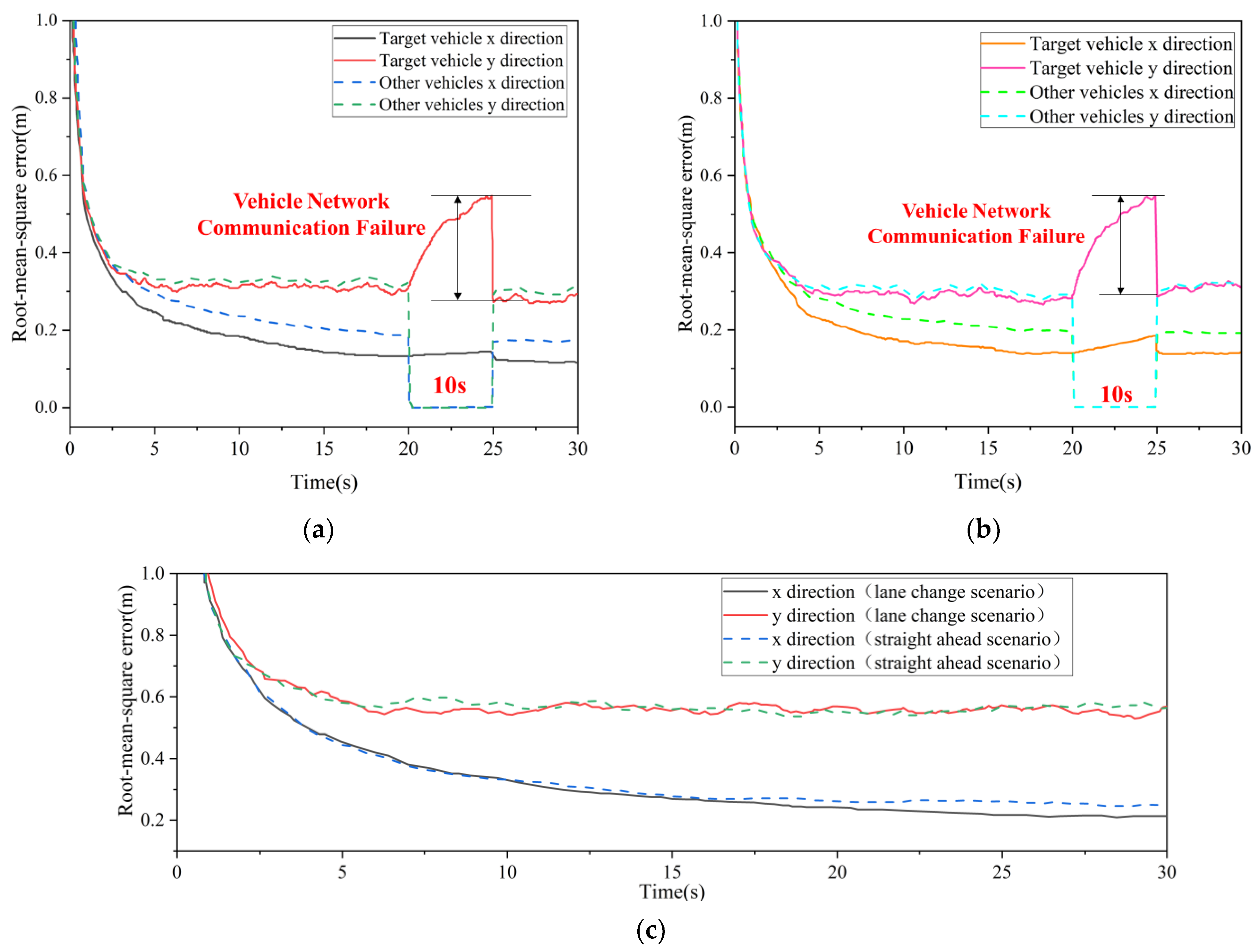
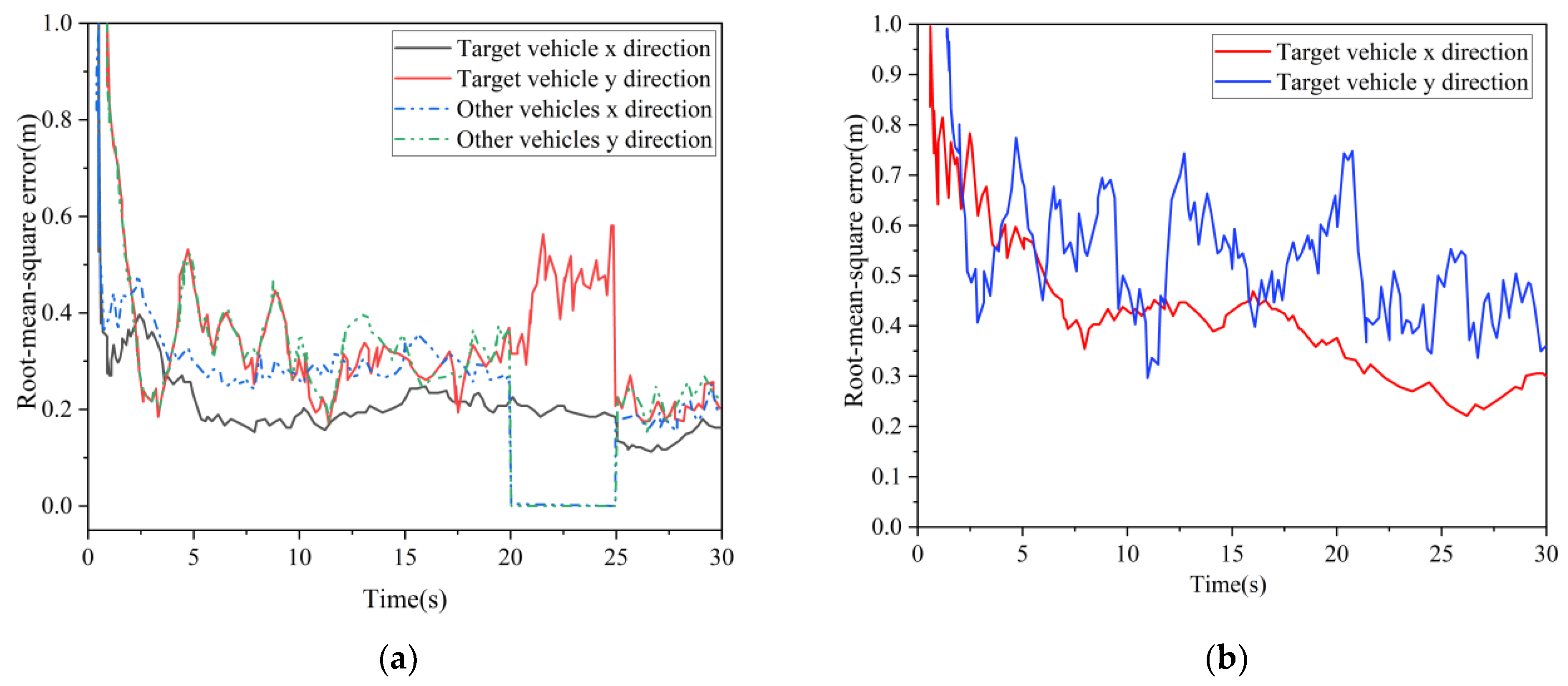
Figure 1. Different methods of vehicle positioning.
Electronics 11 03247 g001
Figure 2. Satellite positioning principle.
Electronics 11 03247 g002
Figure 3. The characteristics of several sensors.
Electronics 11 03247 g003
Figure 4. Vehicle network communication architecture.
Electronics 11 03247 g004
Figure 5. Multi-vehicle cooperative positioning process.
Electronics 11 03247 g005
Figure 6. (a) Interrelationship between the vehicles; (b) Vehicle motion model.
Electronics 11 03247 g006
Figure 7. (a) Straight line simulation scenario; (b) Acceleration variation curve.
Electronics 11 03247 g007
Figure 8. (a) Lane change simulation scenario; (b) Lane change steering angle model; (c) Lateral position curve for lane change motion; (d) Car 2 and Car 9 for lane change simulation.
Electronics 11 03247 g008
Figure 9. (a) Multi-vehicle cooperative positioning errors in lane change scenarios; (b) Multi-vehicle cooperative positioning error in straight-ahead scenario; (c) Individual vehicle positioning error.
Electronics 11 03247 g009
Figure 10. Error variation in a particular channel change simulation: (a) Multi-vehicle cooperative positioning error; (b) Individual vehicle positioning error.
Electronics 11 03247 g010
Table 1. The average value of the error in the time domain for the two positioning methods.
MethodLane Change ScenarioStraight Ahead Scenario
Error (m) Co-PositioningSingle PositioningCo-PositioningSingle Positioning
Root mean square error in the x-direction0.200.360.270.38
Root mean square error in y-direction0.360.610.340.62
Total root mean square error0.420.730.440.74
Publisher’s Note: MDPI stays neutral with regard to jurisdictional claims in published maps and institutional affiliations.

