Short-Term Load Forecasting with an Ensemble Model Based on 1D-UCNN and Bi-LSTM

Abstract

Short-term load forecasting (STLF), especially for regional aggregate load forecasting, is essential in smart grid operation and control. However, the existing CNN-based methods cannot efficiently extract the essential features from the electricity load. The reason is that the basic requirement of using CNNs is space invariance, which is not satisfied by the actual electricity data. In addition, the existing models cannot extract the multi-scale input features by representing the tendency of the electricity load, resulting in a reduction in the forecasting performance. As a solution, this paper proposes a novel ensemble model, which is a four-stage framework composed of a feature extraction module, a densely connected residual block (DCRB), a bidirectional long short-term memory layer (Bi-LSTM), and ensemble thinking. The model first extracts the basic and derived features from raw data using the feature extraction module. The derived features comprise hourly average temperature and electricity load features, which can capture huge randomness and trend characteristics in electricity load. The DCRB can effectively extract the essential features from the above multi-scale input data compared with CNN-based models. The experiment results show that the proposed method can provide higher forecasting performance than the existing models, by almost 0.9–3.5%.

1. Introduction

Accurate load forecasting is vital for the power grid’s operation stability, such as generating units’ scheduling, safety assessment, and reliability analysis [1,2]. With the development of the power system and the integration of renewable energy, it is essential to obtain accurate load forecasting results [3,4].

Load forecasting is categorized into three classes: long-term load forecasting (LTLF), medium-term load forecasting (MTLF), and short-term load forecasting (STLF) [5]. LTLF and MTLF are applied for forecasting the electricity load from several weeks to a few years [6], which are crucial for long-term power generation scheduling and seasonable electricity load analysis [7]. In comparison, STLF ranges from several minutes to a few days. It is crucial for the daily operation of the power grid. It is worth noting that most electricity load series have apparent periodicity.

Nevertheless, the holiday effect and major emergencies also bring random fluctuations to the electricity load, limiting the forecasting efficiency. Therefore, many researchers have designed various STLF models to address this restriction. The existing load forecasting approaches are categorized into statistical and machine-learning-based models. For those data with fixed patterns, the statistical-learning-based methods can execute quickly and provide accurate forecasts. Mbamalu et al. [8] proposed the auto-regressive (AR) model to forecast the electricity load. Moreover, the suboptimal least square method was used to estimate the model parameters and improve model generalization. Kuang et al. [9] dealt with the STLF using the adaptive auto-regressive moving average (ARMA) model. However, AR and ARMA need the stationary input series, which is counterfactual to the actual input data. As a solution, Wang et al. [10] adopted the auto-regressive integrated moving average (ARIMA) in which the integral part transforms the time series, making it stationary. Hence, it can relieve the problem that the STLF method is slightly strict with the input series.

Another popular model for STLF is based on machine learning. It usually begins with an input feature module that can yield hand-crafted features to construct a mapping between the input data and the output values of the network. In the training process, all the network’s neurons can learn the complex relationship between inputs and outputs with constantly updated parameters. The trained network is tested on the dataset of the other samples to evaluate the generalization capacity. Ceperic et al. [11] first designed a feature extraction module to generate the model input. Then, the input data were fed into the support vector machine (SVM) to produce the final forecasting results. Wu et al. [12] adopted the modified generalized regression neural network for STLF. Moreover, the multi-objective searching method was also used to achieve satisfactory performance. Chen et al. [13] first used the similar-day load as their input data. Then, a wavelet neural network was applied to decompose the input series into different frequency components, which were the input of separate neural networks to obtain the final output.

Although the above methods can produce competitive forecasting performance, researchers need more accurate results. The electricity load data present complicated random patterns, and they are challenging to fit precisely [14]. As a solution, deep learning is a powerful method for the forecasted task, as it has the advantage of nonlinear approximation capability [15,16,17].

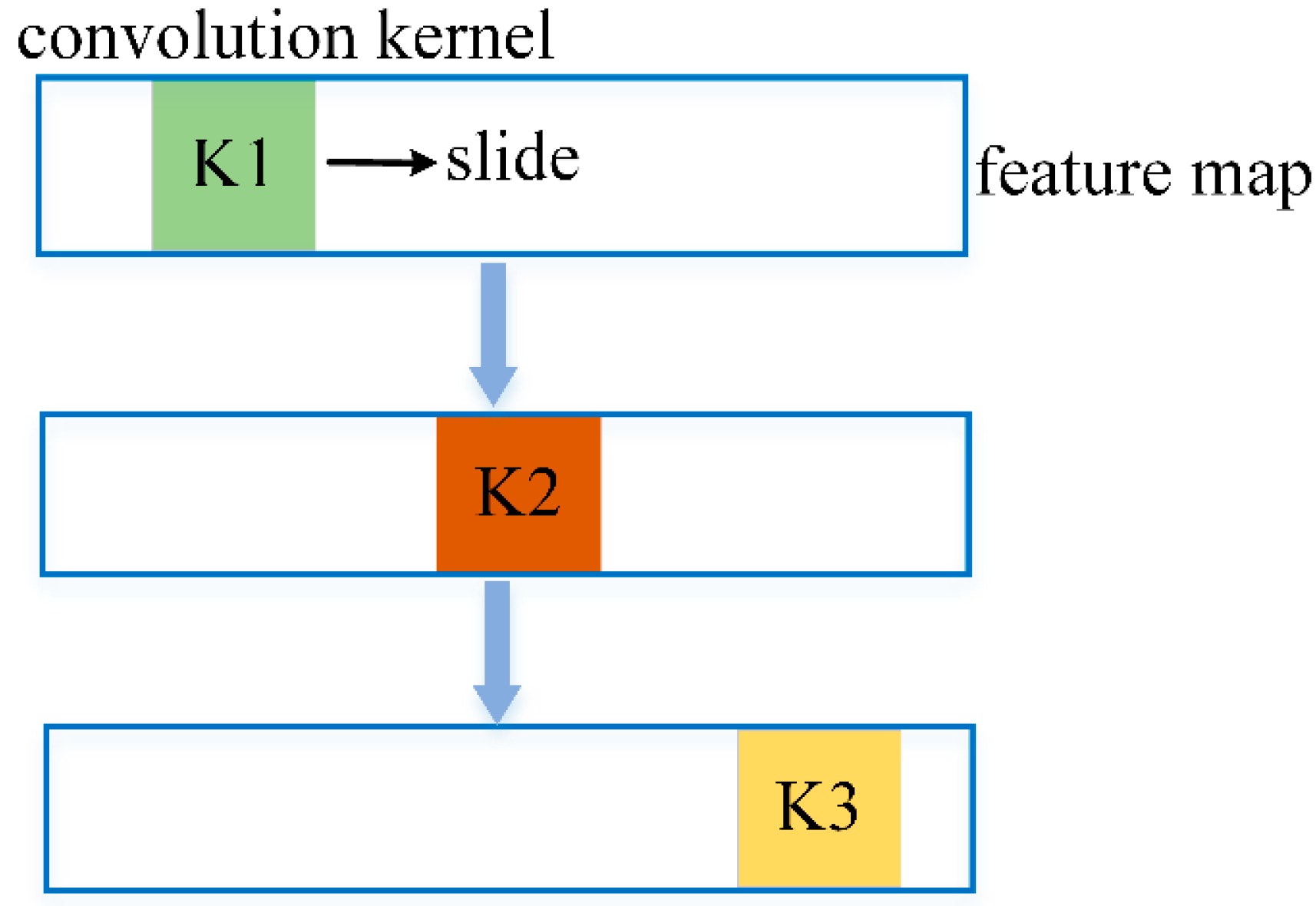
Recently, numerous works based on deep learning have studied STLF. Deng et al. [18] concluded that it is hard to forecast the electricity load precisely. Moreover, a convolutional neural network (CNN) was used to produce competitive results. Dong et al. [19] adopted the K-means algorithm to cluster a large dataset into a few subsets. Then, they were fed into a CNN to obtain the final forecasting result. However, the STLF models based on CNNs still have some limitations. Specifically, the basic requirement of adopting CNNs is space invariance [20], which cannot be satisfied by the actual load data (we detail this problem in Section 3 of this work). Another commonly used method is the long short-term memory network (LSTM). Tan et al. [21] developed an ensemble network that can integrate multiple LSTMs to forecast the electricity load. Liu et al. [22] indicated that the forecasting model based on those LSTM networks could obtain more accurate forecasting performance than artificial neural networks (ANNs) and ARIMA. However, these studies usually pay attention to extracting the features from different LSTM networks, and the generalization capacity of deep learning has not been fully exploited.

Table 1. Comparison of the proposed model with related papers in the literature.

References	Model	Input Variables	Horizon
[8]	AR	Electricity load, temperature	7 days ahead
[9]	ARMA	Time, electricity load	1 day ahead
[11]	SVM	Season, Temperature, and electricity load	1 h ahead
[12]	GRNN	Electricity load	1 day ahead
[13]	WNN	Time, wind speed, and electricity load	1 day ahead
[19]	K-means, CNN	Electricity load	7 days ahead
[21]	LSTM	Time, electricity load	1 day ahead
Proposed model	UCNN, Bi-LSTM	Season, time, electricity load, and temperature	1 day ahead

shows a comparison between the proposed model and previous works in various aspects, including input features and forecasting horizon.

Overall, the generalization capacity of deep neural networks (DNNs) boosts as the network depth increases. Nevertheless, overfitting and gradient disappearance usually exist and significantly affect DNN performance as the scale of the DNN increases. Two methods have been applied to relieve this limitation: improving the layer itself and modifying the structure of the DNN. A common approach for the first method is the bidirectional long short-term memory network (Bi-LSTM) [23]. Compared with LSTM, Bi-LSTM can train the network parameters in different directions, boosting the performance of time series learning. Toubeau et al. [24] demonstrated that Bi-LSTM networks could yield significantly improved results compared with LSTM networks. The second method is based on residual learning, which transforms the structure of the DNN by adding shortcut connections [25]. In addition, different residual learning variants have been proposed and achieved high performance [26,27]. Thus, the proposed model adopts hourly electricity load and temperature to forecast the electricity load on the following day. Specifically, the contributions of this study are summarized as follows:

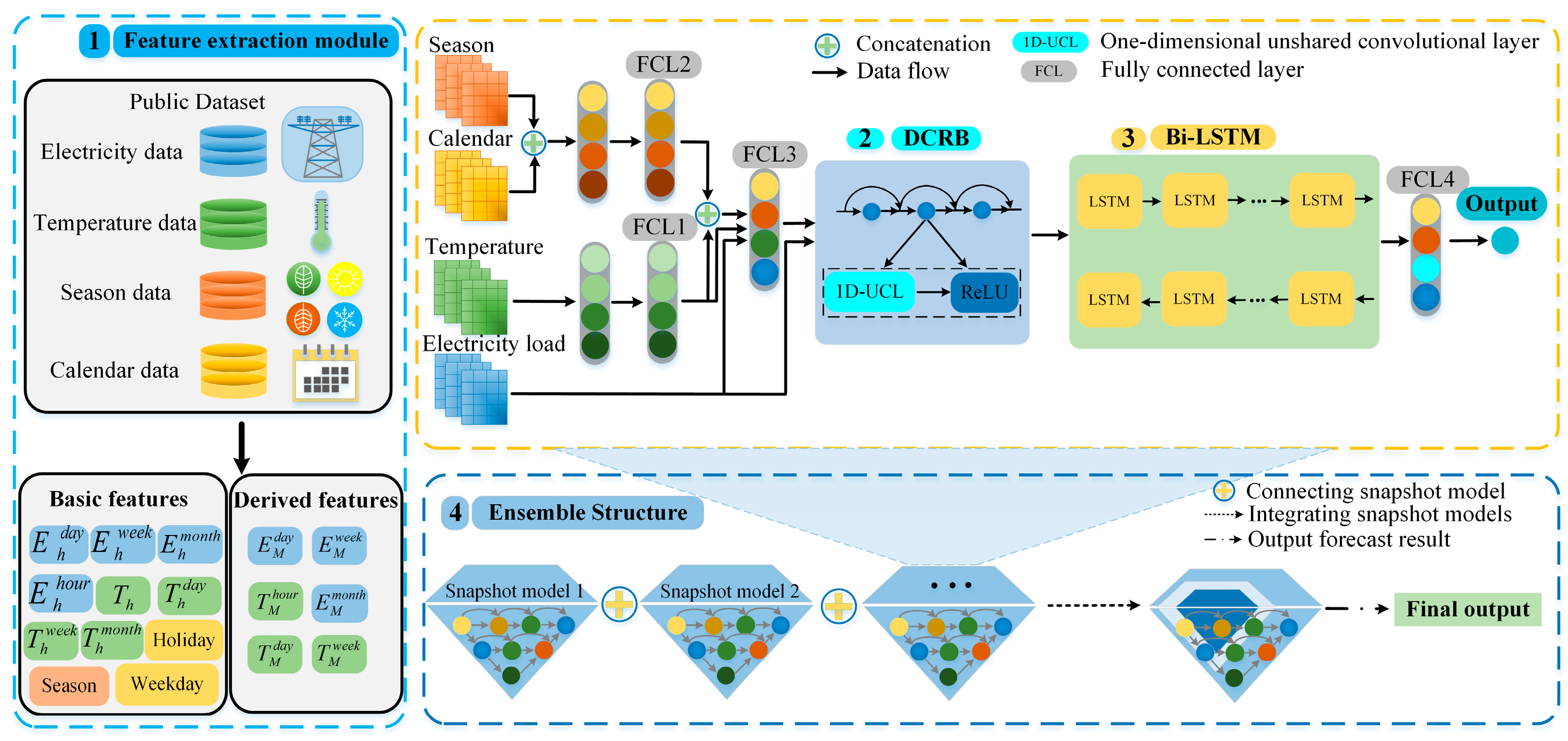
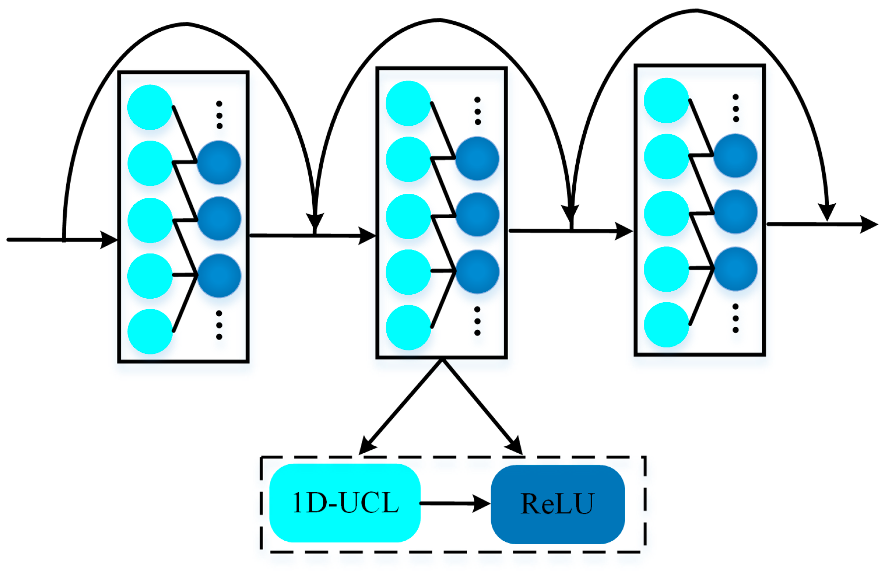
• We designed a densely connected residual block (DCRB) based on an unshared convolutional layer (UCL), which can effectively relieve over-fitting and gradient disappearance;
• We proposed a novel ensemble method for deterministic electricity load forecasting. The model includes a one-dimensional unshared convolutional neural network (1D-UCNN) and a bidirectional long short-term memory layer (Bi-LSTM). In addition, the generalization ability of the proposed model was verified by testing it on two benchmark datasets.

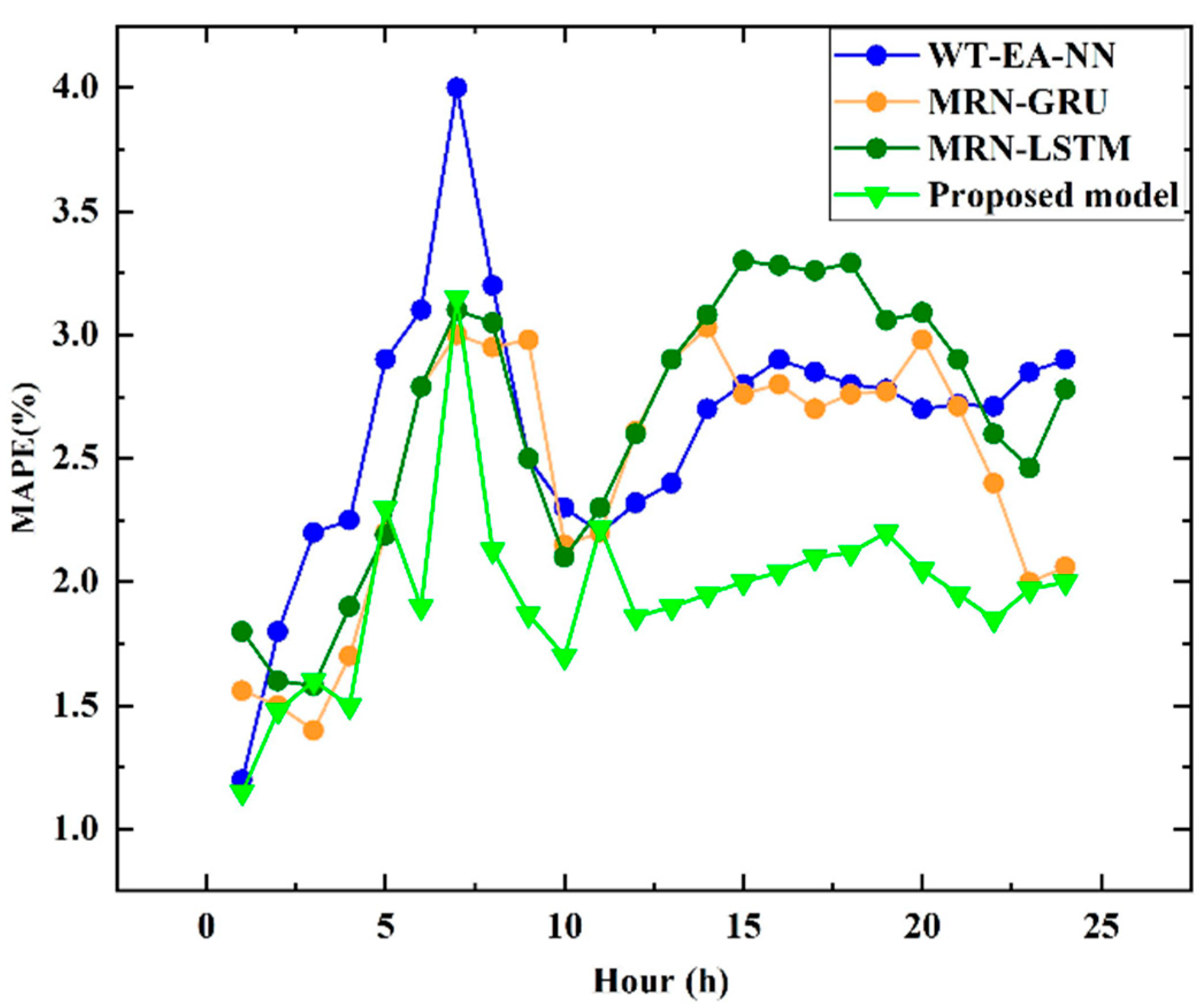
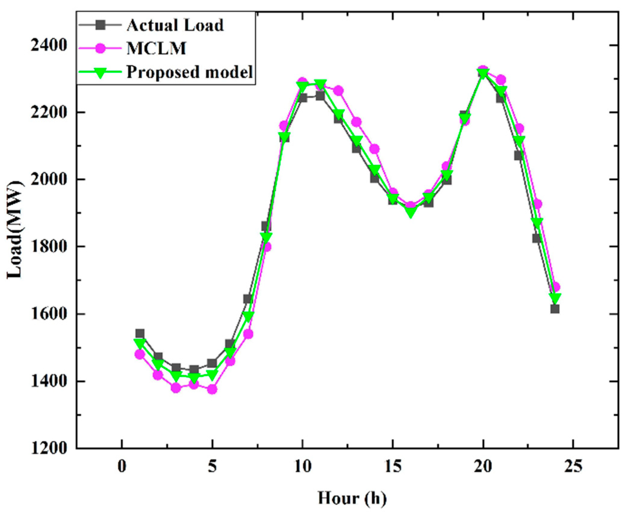
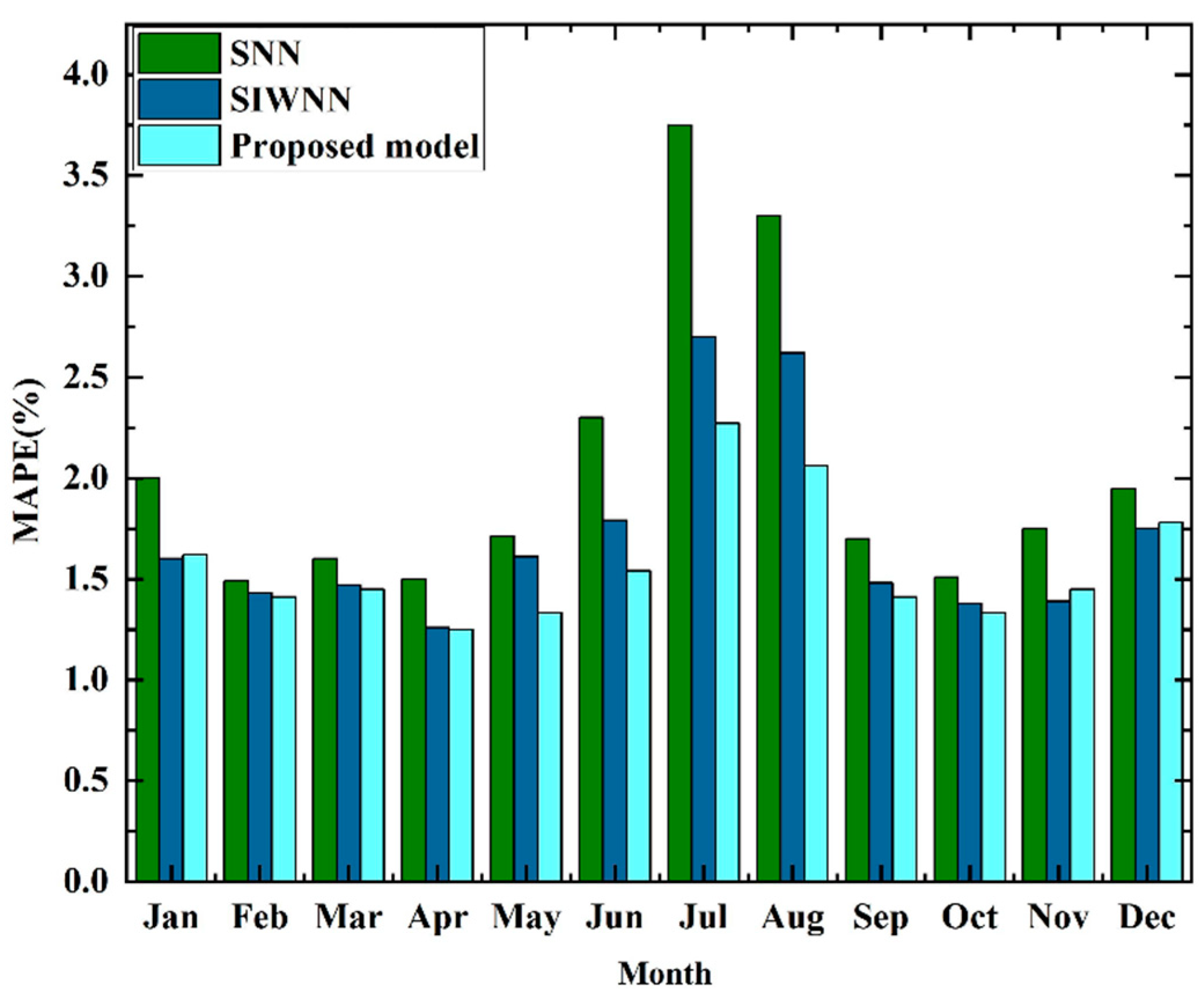
The rest of the paper is organized as follows: Section 2 introduces the overall framework of the proposed ensemble model, which consists of a feature extraction module, a densely connected residual block (DCRB), Bi-LSTM, and the ensemble structure. Section 3 shows the experiment results and demonstrates the performance comparison of the proposed method on two public datasets from North America and New England. Finally, the conclusions and future research direction are drawn in Section 4.

2. Method

2.1. Overall Framework

In this paper, we designed a flexible framework to forecast the short-term electricity load, as shown in Figure 1. In addition, its backbone is based on a DCRB and Bi-LSTM layer. At first, the input data are preprocessed to obtain the basic and derived features by the virtue of the feature extraction module. Specifically, the derived features comprise the average electricity features and temperatures. The temperature features are first concatenated and sent as input to two separate fully connected layers, with the second layer representing FCL1. The model also concatenates the calendar features and connects them with two fully connected layers. The second layer represents FCL2. Moreover, the model continues concatenating FCL1, FCL2, the actual temperature, and the electrical loads over one day. They are further connected with a separate fully connected layer denoted as FCL3, which is concatenated with other electricity load features. Then, the DCRB extracts the essential features from the above input data. The following Bi-LSTM layer can further capture the hidden temporal pattern. The forecasting value of one snapshot by a dense layer with is obtained with the linear activation function. In addition, the proposed model can construct multiple snapshots and ensemble them through ensemble thinking. The proposed framework produces the final forecasting result after averaging the snapshots’ outputs.

2.2. Feature Extraction

Input features are essential in accurate electricity forecasting performance [6]. Hence, in this study, we divided the input data into the basic and derived features, which are represented by Basic(h) and Derived(h), respectively; h is calculated hourly, and the reason is that we studied hourly load. Specifically, Basic(h) and Derived(h) can be listed as follows:

$$\left[\begin{array}{c}{E}_h^{hour}(h\text{-}1),\dots ,E_h^{hour}(h\text{-}24)\\ E_h^{day}(h\text{-}24),\dots ,E_h^{day}(h\text{-}168)\\ E_h^{week}(h\text{-}168),\dots ,E_h^{week}(h\text{-}672)\\ E_h^{month}(h\text{-}672),E_h^{month}(h\text{-}1344),E_h^{month}(h\text{-}2016)\\ T_h^{day}(h\text{-}24),\dots ,T_h^{day}(h\text{-}168)\\ T_h^{week}(h\text{-}168),\dots ,T_h^{week}(h\text{-}672)\\ T_h^{month}(h\text{-}672),T_h^{month}(h\text{-}1344),T_h^{month}(h\text{-}2016)\\ Season(h),Weekday(h),Holiday(h)\end{array}\right]$$

(1)

$$\left[\begin{array}{c}{E}_M^{day}(h),E_M^{week}(h),E_M^{month}(h)\\ T_M^{day}(h),T_M^{week}(h),T_M^{month}(h),T_h\end{array}\right]$$

(2)

The basic features consist of electricity load, temperature, season, and calendar information. In addition, the derived features are obtained by calculating the basic ones. More precisely, the derived features include a series of average values concerning the load and temperature. These two types of input features are crucial for STLF. As shown in

Table 2. Input data for the load forecast of the $h^{th}$ hour.

Symbol	Size	Description of the Inputs
$E_h^{hour}$	24	Electricity values within 24 h before the $h^{th}$ hour
$E_h^{day}$	7	Electricity values of the $h^{th}$ hour of every day within a week
$E_h^{week}$	4	Electricity values of the $h^{th}$ hour of days 7, 14, 21, and 28 before the forecasted day
$E_h^{month}$	3	Electricity values of the $h^{th}$ hour of days 28, 56, and 84 before the forecasted day
$E_M^{day}$	1	The average value of $E_h^{day}$
$E_M^{week}$	1	The average value of $E_h^{week}$
$E_M^{month}$	1	The average value of $E_h^{month}$
$T_h$	1	The actual temperature of the $h^{th}$ hour
$T_h^{day}$	7	Temperatures of the $h^{th}$ hour of every day within a week
$T_h^{week}$	4	Temperatures of the $h^{th}$ hour of days 7, 14, 21, and 28 before the forecasted day
$T_h^{month}$	3	Temperatures of the $h^{th}$ hour of days 28, 56, and 84 before the forecasted day
$T_M^{day}$	1	The average value of $T_h^{day}$
$T_M^{week}$	1	The average value of $T_h^{week}$
$T_M^{month}$	1	The average value of $T_h^{month}$
$Season$	4	One-hot encoding for season
$Weekday$	2	One-hot encoding for weekday/weekend
$Holiday$	2	One-hot encoding for holiday

, the basic load features, such as $E_h^{hour}$, $E_h^{day}$, $E_h^{wek}$, and $E_h^{month}$, are added to capture the long/short-term trends of the load series. Furthermore, the basic temperature features, such as $T_h$, $T_h^{day}$, $T_h^{wek}$, and $T_h^{month}$, can reflect the effect of the long/term-term temperature change trend on the load. The seasonal feature, Season(h), is added to track certain seasonal regularity in the load series. The calendar features, such as $Weekday(h)$ and $Holiday(h)$, can make it easier for the proposed method to capture the weekday effect and the dynamic characteristics influenced by holidays. The derived features, such as $E_M^{day}$, $E_M^{week}$, $E_M^{month}$, $T_M^{day}$, $T_M^{week}$, and $T_M^{month}$, are added to further capture the random fluctuation of long-/short-term trends in the load series and the effect of the temperature change on the electricity load.

2.3. Densely Connected Residual Block

Previous studies usually adopted FCN and one-dimensional convolutional neural network (1D-CNN)-based deep learning models to forecast the short-term electricity load [15,28]. Nevertheless, these methods have some limitations. Specifically, FCN usually suffers from over-fitting and gradient disappearance with many parameters. In addition, 1D-CNNs demand that the space of input data be invariant, but the electricity load data are virtually space-variant. We introduce this problem in Section 3.

Therefore, in this paper, we proposed a densely connected residual block (DCRB) by introducing the residual fashion into a one-dimensional unshared convolutional layer, as shown in Figure 2. The proposed DCRB can address the above issues. Unlike FCN, over-fitting and gradient disappearance are unlikely to occur due to its fewer parameters. Compared with 1D-CNNs, its convolution kernel parameters with respect to the various positions of input feature mapping are not shared. The reason is that 1D-UCNN does not require space invariance for input data. This section further introduces the implementation details of the DCRB. The training dataset is given as follows:

$$D={\{{\mathrm{x}}_{\mathrm{i}},{\mathrm{y}}_{\mathrm{i}}\}}_{t=i}^n$$

(3)

where ${\mathrm{x}}_{\mathrm{i}}$ denotes the $i^{th}$ training data, and ${\mathrm{y}}_{\mathrm{i}}$ is the corresponding value. The output of the model Θ (${\mathrm{x}}_{\mathrm{i}}$) converges to ${\mathrm{y}}_{\mathrm{i}}$ after several training iterations. Θ ($·$) denotes the 1D-UCNN model. As shown in Figure 3, the region contained in the blue border denotes a feature map. Moreover, the squares represent the convolution kernels, which slide across the feature map to extract essential features. The three convolution kernels are marked in various colors, and they denote the different weight parameters. The feature extraction process of the $l^{th}$ hidden layer is expressed as follows:

$$o_t^l=\psi (h_t^{l-1})$$

(4)

where $h_t^{l-1}$ stands for the $t^{th}$ convolution area at ${(l-1)}^{th}$ layer, $o_t^l$ represents the convolutional output, and $\psi$($·$) is the unshared convolution operator. Moreover, the outputs corresponding to the various convolutional areas are concatenated as new features, which are separated as different convolutional areas for the following convolution operation.

It is worth noting that the 1D-UCNN layer is introduced into the residual architecture to strengthen the generalization ability of the network. Specifically, the gradient information could back-propagate by adding the shortcut connections. Specifically, the $l^{th}$ hidden layer’s output is formulated as follows:

$$o_t^l=\psi (h_t^{l-1})+h_t^{l-1}$$

(5)

Then, the DCRB structure is established as shown in Figure 3. It is vital a component of the proposed model. The DCRB can effectively capture essential information from the electricity load series through a densely residual fashion.

2.4. Bidirectional Long Short-Term Memory (Bi-LSTM)

Though the traditional STLF models, such as ARIMA and ANN, can learn the time series data, their forecasting performance is not excellent. The reason is that they do not fully consider the long-term temporal dependence in the time series data. As a solution, an LSTM model is used to overcome the above limitation [29,30,31].

Specifically, the LSTM unit is composed of four essential components, which can make it easier to learn the long-dependence features. In addition, its computing process is formulated as follows:

$$g_t=\sigma (U^{(g)}{x}_t+W^{(g)}{h}_{t-1}+b_g)$$

(6)

$$f_t=\sigma (U^{(f)}{x}_t+W^{(f)}{h}_{t-1}+b_f)$$

(7)

$$q_t=\sigma (U^{(q)}{x}_t+W^{(q)}{h}_{t-1}+b_q)$$

(8)

$$\tilde{s} =tanh (U^{(c)}{x}_t+W^{(q)}{h}_{t-1}+b_q)$$

(9)

$$s_t=f_t\circ s_{t-1}+g_t\circ \tilde{s}$$

(10)

$$h_t=g_t\circ tanh(s_t)$$

(11)

where $g_t$ denotes the gate for receiving the input data. $f_t$ denotes the forget gate, and it determines the amount of information that can be discarded. $q_t$ denotes the output gate, which determines how much information should be transmitted to the output layer. $\tilde{s}$ is the self-recurrent unit similar to a recurrent neural network (RNN). $s_t$ is an internal memory unit of each LSTM cell, which is composed of two parts. Specifically, the first term represents the calculation result of the previous state $s_{t-1}$ and forget gate $f_t$. The second term is obtained by calculating state $\tilde{s}$ and input gate g_t. $h_t$ is the hidden state of the LSTM.

The disadvantage of the LSTM is that it can only learn the previous information of the time series data. As a solution, a Bi-LSTM model is proposed to deal with the sequence data in different directions through a forward layer and a backward layer. Specifically, the functions of the Bi-LSTM layers are formulated as follows:

$${\overrightarrow{h}}_t=\sigma ({\overrightarrow{U}}^{(g)}{\overrightarrow{x}}_t+{\overrightarrow{W}}^{(g)}{\overrightarrow{h}}_{t-1}+{\overrightarrow{b}}_g)$$

(12)

$${\overrightarrow{f}}_t=\sigma ({\overrightarrow{U}}^{(f)}{\overrightarrow{x}}_t+{\overrightarrow{W}}^{(f)}{\overrightarrow{h}}_{t-1}+{\overrightarrow{b}}_f)$$

(13)

$${\overrightarrow{q}}_t=\sigma ({\overrightarrow{U}}^{(q)}{\overrightarrow{x}}_t+{\overrightarrow{W}}^{(q)}{\overrightarrow{h}}_{t-1}+{\overrightarrow{b}}_q)$$

(14)

$$\overrightarrow{\tilde{s} }=tanh ({\overrightarrow{U}}^{(c)}{{\overrightarrow{x}}_t}_t+{\overrightarrow{W}}^{(c)}{\overrightarrow{h}}_{t-1}+{\overrightarrow{b}}_c)$$

(15)

$$\overrightarrow{s_t}=\overrightarrow{f_t}\circ {\overrightarrow{s}}_{t-1}+\overrightarrow{l_t}\circ \overrightarrow{\tilde{s} }$$

(16)

$${\overrightarrow{h}}_t={\overrightarrow{q}}_t\circ tanh(\overrightarrow{s_t})$$

(17)

$${\overleftarrow{h}}_t=\sigma ({\overleftarrow{U}}^{(g)}{\overleftarrow{x}}_t+{\overleftarrow{W}}^{(g)}{\overleftarrow{h}}_{t-1}+{\overleftarrow{b}}_g)$$

(18)

$${\overleftarrow{f}}_t =\sigma ({\overleftarrow{U}}^{(f)}{\overleftarrow{x}}_t+{\overleftarrow{W}}^{(f)}{\overleftarrow{h}}_{t-1}+{\overleftarrow{b}}_f)$$

(19)

$${\overleftarrow{q}}_t=\sigma ({\overleftarrow{U}}^{(q)}{\overleftarrow{x}}_t+{\overleftarrow{W}}^{(q)}{\overleftarrow{h}}_{t-1}+{\overleftarrow{b}}_q)$$

(20)

$$\overleftarrow{\tilde{s}}=tanh ({\overleftarrow{U}}^{(c)}{\overleftarrow{x}}_t+{\overleftarrow{W}}^{(c)}{\overleftarrow{h}}_{t-1}+{\overleftarrow{b}}_c)$$

(21)

$${\overleftarrow{s}}_t=\overleftarrow{f_t}\circ {\overleftarrow{s}}_{t-1}+{\overleftarrow{l}}_t\circ \overleftarrow{\tilde{s}}$$

(22)

$${\overleftarrow{h}}_t={\overleftarrow{q}}_t\circ tanh ({\overleftarrow{s}}_t)$$

(23)

$$h_t={\overrightarrow{h}}_t\circ {\overleftarrow{h}}_t$$

(24)

where the oppositely oriented arrows mean the forward and backward propagation of the data, respectively. Meanwhile, $h_t$ denotes the status of the Bi-LSTM at time t, which is obtained by connecting the forward propagation output ${\overrightarrow{h}}_t$ and the backward propagation output ${\overleftarrow{h}}_t$. Hence, the Bi-LSTM can learn the essential information from past and future time series data and obtain the final output.

2.5. Ensemble Structure

The machine learning field widely accepts that ensemble models can provide more accurate forecasting results than single ones [32,33]. Thus, the adopted ensemble thinking in this paper can be divided into two stages. Several snapshot models are firstly saved during the training process of an independent model. Specifically, we adopted the adaptive moment estimation (Adam) [34] to optimize the independent model. Hence, the model can adjust the learning rate during the various training stages. Then, several snapshots are saved following the proposed approach in [35].

Next, several independent models are further trained, which are the basis for integrating the precise models. Following [36], the parameters are reinitialized to obtain a few independent models. Thus, in this paper, we considered the number of snapshots saved during a training period and independent models as hyperparameters. Specifically, Section 3 details its confirmation process. The final output of the model is the average value of all the snapshots.

3. Experiment Results

3.1. Test Settings

This study shows the one-day-ahead electricity load forecasting on two public datasets from New England and North America. Both datasets comprise hourly historical loads and temperatures. The historical data were divided into a training set, a validation set, and a test set. Specifically, the training set was applied to update the model parameters. The validation set confirmed the best hyperparameters. The data were normalized as the preprocessing step in this paper. The electricity load data and the temperature data were normalized in the range of [0, 1], which could speed up the convergence of the model. The MAPE values of the existing models and the proposed model were obtained in a day, week, month, and year for a fair comparison. It is worth noting that the forecasting results of the compared methods were directly from related studies. In addition, the experiments were implemented on a laptop with an Intel core i7-4500U processor. Keras 2.3.0 backend in the Python 3.6 environment was applied for all the experiments.

3.2. Results of the North American Dataset

The proposed framework was first applied to a public dataset from North American Utility, including 57 months. In addition, the dataset was divided into three subsets with a split ratio of 0.6/0.1/0.3. Specifically, the period was from 1 January 1988 to 12 October 1992. The data from 1 January 1988 to 31 December 1990 were for training, and the data from 1 January 1991 to 12 October 1992 were for testing. The validation set ranged from 1 January 1990 to 31 December 1990.

First, we tested the influence of different hyperparameters on forecasting accuracy. Concretely, the tuned hyperparameters were determined by the number of independent models and snapshots saved in a single training process. The performance comparison with the different number of snapshots is shown in Figure 4. It can be observed that the proposed ensemble framework provided the lowest forecasting error when the four snapshots were saved, respectively, during the training process of the three independent models.

For further evaluation of forecasting performance, we compared the proposed framework with WT-NN [37], WT-EA-NN [38], ESN [39], and MCLM [40]. Moreover, we also evaluated the influence of the possible errors in forecasting temperatures over the generalization performance of the model, as shown in

Table 3. Performance comparison of MAPEs on the data of North American dataset during 1991 and 1992.

Model	Actual Temperature	Noisy Temperature
WT-NN [37]	2.64	2.84
WT-EA-NN [38]	2.04	-
ESN [39]	2.37	2.53
MCLM [40]	2.17	2.25
Proposed model	1.96	2.01

. Concretely, this case added Gaussian noise with a mean of 0 °F and a standard deviation of 1 °F to the actual temperature for a fair comparison with the benchmark models. Then, the comparative analysis of the state-of-the-art models and the proposed model was carried out as follows:

WT-NN [37] and WT-EA-NN [38] are hybrid models based on wavelet transform (WT). The WT-NN [37] model comprises WT and neural networks (NNs). Different from WT-NN [37], WT-NN-EA [38] method firstly decomposes the hourly electricity load data into different frequency components using the wavelet transform (WT). Then, they are fed into a composite framework consisting of NNs and an evolutionary algorithm (EA) to produce the forecasting result. As shown in Table 3, the proposed method performed 25.8% and 3.9% better in the actual temperature case than WT-NN [37] and WT-EA-NN [38], respectively. When considering the noise temperature, its forecasting performance improved by 29.2%. Therefore, the proposed model is more competitive in the field of STLF.

ESN [39] denotes the echo state network (ESN), which is one of the RNNs used to forecast the electricity load. Its input variables are based on basic features, such as electricity load, temperature, season, and calendar information. Compared with ESN [39], the forecasting accuracy of the proposed method improved by 17.2% for actual temperature conditions and 20.5% for noise temperature conditions. Such improved performance shows that the Bi-LSTM used in the proposed method is a more efficient component to capture the dynamic characteristics of the electricity load series.

In addition, MCLM [40] method adopts multiple CNNs and LSTMs for STLF. With the actual temperature case, the proposed method surpassed the MCLM [40] by 9.6% on the index of MAPE. Moreover, the forecasting accuracy improved by 10.7% in the noisy temperature data. The experimental results show that the proposed method based on 1D-UCNN outperformed the CNN-based method, and the proposed framework was more flexible for temperature variation.

We further compared the forecasting results of the proposed method with other deep learning methods, such as WT-EA-NN [38], MRN-LSTM [41], and MRN-GRU [41]. MRN-LSTM [41] first adopts the load and temperature features as the input data of multiple fully connected layers. Then, the preliminary forecasted value is fed to the LSTM layer to obtain the final output. MRN-GRU [41] is carried out by combing multiple fully connected layers and a GRU layer. The forecasting results are shown in Figure 5 and Figure 6. At 1 a.m., the electricity loads concerning the previous 24 h of the method were the actual data. Thus, the proposed method produced the best forecasting results. At 7 a.m., the forecasting deviation reached the maximum, and the MAPE was 2.21. In addition, the proposed model could achieve more accurate one-day forecasting results, compared with the other models, for most months.

3.3. Results of the New England Dataset

In the second experiment, we used the New England dataset to test the generalization ability of the proposed framework. Specifically, the dataset comprised the hourly electricity loads and temperature data from 1 March 2003 to 31 December 2014. In addition, for this experiment, adopted the same hyperparameters tuned with the North American dataset to train the STLF model for a fair comparison with the benchmark models. The New England dataset was divided into two subsets with a split ratio of 0.75/0.25 for case 1 and 0.6/0.4 for case 2. The first case was adopted to test the forecasting results from 1 January 2006 to 31 December 2006, and the period of the training set was from 1 March 2003 to 31 December 2005. The training set of the second case was from 1 January 2003 to 31 December 2009, and the testing set was from 1 January 2010 to 31 December 2011.

In the first case, we compared the proposed model with SNN [13] and SIWNN [13]. SNN [13] is implemented using a single neural network, which adopts the calendar information, electricity load, and temperature data as the input. In comparison, SIWNN [13] selects a similar day load as the input. Separate neural networks extract the load feature processed by wavelet decomposition. As shown in Figure 7, the proposed model could produce lower forecasting errors than the other models in most months over one year.

The second case provided a comparison between the generalization ability of the proposed method and those of the state-of-the-art models mentioned in [41,42,43], as shown in

Table 4. Performance comparison of MAPEs on the data of New England dataset during 2010 and 2011.

Model	2010	2011
CNN	3.78	3.93
ErrCorr-RBF [42]	1.80	2.02
MErrCorr-RBF [43]	1.75	1.98
MRN [41]	1.50	1.80
Proposed model	1.49	1.78

. A CNN was selected for the basic comparison, which is because it is a common module of the deep learning method. Specifically, the CNN had a convolutional layer and four fully connected layers. The number of convolutional filters was eight, and the size of the convolutional kernel was one. ErrCorr-RBF [42] is an offline network based on the radial basis function (RBF). The RBF is applied to fit the actual electricity load data during the training process of an error correction (ErrCorr) algorithm, reducing the forecasting error. MErrCorr-RBF [43] further integrates the input data pruning process in the learning stage, which can help the model produce more accurate forecasting results. In addition, MRN [41] denotes a modified residual network (MRN) where the added shortcuts and residual blocks boost the model generalization. As shown in Table 4, the proposed model could obtain the most accurate forecasting results. For instance, the proposed framework achieved 1.50% and 1.78% for the years 2010 and 2011, respectively. In comparison, the forecasting performance of the existing models was much worse. Specifically, the MAPE values corresponding to ErrCorr-RBF [42], MErrCorr-RBF [43], and MRN [41] were 1.80%, 1.75%, and 1.50% for the year 2010 and 2.02%, 1.98%, and 1.80% for the year 2011, respectively. Note that the proposed model, which is based on one-dimensional unshared convolution, could provide more accurate forecasting performance than the classic convolution-based method.

The generalization ability of the methods based on the CNN was worse, and the reason is that classic convolutional kernels require the input data to be space-invariant [20]. However, the electricity load data are virtually space-variant. Specifically, Figure 8 presents how the input data batch for STLF was constructed as a matrix. The data of each row denote the timestamp. The data of the column comprise multi-scale load features, temperature, and calendar information. For the same timestamp, the various categories of the input feature provide different information, which is named feature imbalance. Additionally, the data concerning the various timestamp comprise different information, which could have various impacts on the model generalization. This is known as time imbalance. The imbalance between the input data of different categories and timestamps results in an imbalanced condition between rows and columns, which means space variance. Obviously, the electricity load data cannot be satisfied with the requirement of classic convolutional kernels. Thus, the proposed model could outperform the classic convolution-based ones without the requirement of space invariance. Then, we evaluated the forecasting performance of the proposed method using the MAPE performance index of each day within a week, as indicated in Figure 9. The visual comparison demonstrates that ensemble thinking can boost the generalization performance of the method.

As we adopted the actual temperature data as the model input, the forecasting results show the estimated upper bound of the forecasting performance. It is essential to analyze the forecasting accuracy of the proposed model when the forecasted temperature was adopted, and whether ensemble thinking can help the model produce more robust results in noisy temperature conditions. Thus, we adopted the method of modifying the temperature data proposed in [36] and designed three cases to verify the generalization ability of the proposed method. We repeated the experiments 5 times and obtained the means of increased MAPE and computation time.

The increased MAPEs concerning the year 2010 in noise temperature conditions are indicated in Figure 8. Specifically, we compared the generalization ability of the proposed ensemble method (which consists of thirteen snapshot models) with a single snapshot trained with 1300 epochs. As shown in Figure 10, ensemble thinking could obviously reduce the increase in MAPE value. Specifically, the increased MAPE value was 0.027% in case 1. In addition, the smallest increased MAPE value for case 1 was 0.05%. In addition, the average computation time for the proposed ensemble method was 18.77 s, and it was slightly worse than the proposed model without ensemble thinking, with a mean value of 12.94 s, as shown in

Table 5. Comparison of computation time concerning the proposed model with ensemble thinking and the proposed model without ensemble thinking.

Case	With Ensemble	Without Ensemble
Case 1	18.78 s	12.93 s
Case 2	18.80 s	12.91 s
Case 3	18.75 s	12.98 s

. The reason is that the proposed ensemble model needs to construct multiple snapshots and ensemble them. Despite having a single model with less computation time, the forecasting accuracy of the proposed ensemble model was better, especially in case 3. Thus, the experiment results show that the proposed method still obtained accurate forecasting results in noisy temperature conditions, and ensemble thinking could improve model generalization.

4. Conclusions

Load forecasting plays an essential role in the management of power systems, and it can relieve the limitations caused by the lack of electricity. In this paper, we designed a novel ensemble model with multiple snapshots to forecast the short-term electricity load. Each snapshot comprised multiple separate fully connected layers, a DCRB, and a Bi-LSTM layer. In addition, the experimental results indicate that the proposed method had higher forecasting accuracy than the existing models, and the maximum improvement was up to 3.5% in MAPE. In future work, different deep learning methods will be investigated to leverage their forecasting advantages. In addition, simulations on optimizing the Bi-LSTM neural network parameters will be performed to construct a more accurate model. We also plan to analyze the different factors affecting the electricity load to better learn the time series load data.

References

1. Wu, L.; Shahidehpour, M. A hybrid model for day-ahead price forecasting. IEEE Trans. Power Syst. 2010, 25, 519–1530. [Google Scholar]
2. Abedinia, O.; Amjady, N.; Zareipour, H. A new feature selection technique for load and price forecast of electrical power systems. IEEE Trans. Power Syst. 2017, 32, 62–74. [Google Scholar] [CrossRef]
3. Chen, X.; Hou, Y.; Hui, S.Y.R. Distributed control of multiple electric springs for voltage control in microgrid. IEEE Trans. Smart Grid 2017, 8, 1350–1359. [Google Scholar] [CrossRef]
4. Borges, C.E.; Penya, Y.K.; Fernandez, I. Evaluating combined load forecasting in large power systems and smart grids. IEEE Trans. Ind. Informat. 2013, 9, 1570–1577. [Google Scholar] [CrossRef]
5. Chen, X.; Shi, M.; Sun, H.; Li, Y.; He, H. Distributed cooperative control and stability analysis of multiple DC electric springs in a DC microgrid. IEEE Trans. Ind. Electron. 2018, 65, 5611–5622. [Google Scholar] [CrossRef]
6. Hippert, H.S.; Pedreira, C.E.; Souza, R.C. Neural networks for short-term load forecasting: A review and evaluation. IEEE Trans. Power Syst. 2001, 16, 44–55. [Google Scholar] [CrossRef]
7. Kong, W.; Dong, Z.Y.; Jia, Y.; Hill, D.; Xu, Y.; Zhang, Y. Short-term residential load forecasting based on LSTM recurrent neural network. IEEE Trans. Smart Grid 2019, 10, 841–851. [Google Scholar] [CrossRef]
8. Mbamalu, G.; Hawary, M. Load forecasting via suboptimal seasonal autoregressive models and iteratively reweighted least squares estimation. IEEE Trans. Power Syst. 1993, 8, 343–348. [Google Scholar] [CrossRef]
9. Huang, S.J.; Shih, K.R. Short-term load forecasting via ARMA model identification including non-gaussian process considerations. IEEE Trans. Power Syst. 2003, 18, 673–679. [Google Scholar] [CrossRef] [Green Version]
10. Contreras, J.; Espinola, R.; Nogales, F.J.; Conejo, A.J. ARIMA models to predict next-day electricity prices. IEEE Trans. Power Syst. 2003, 18, 1014–1020. [Google Scholar] [CrossRef]
11. Ceperic, E.; Ceperic, V.; Baric, A. A strategy for short-term load forecasting by support vector regression machines. IEEE Trans. Power Syst. 2013, 28, 4356–4364. [Google Scholar] [CrossRef]
12. Wu, Z.; Zhao, X.; Ma, Y.; Zhao, X. A hybrid model based on modified multi-objective cuckoo search algorithm for short-term load forecasting. Appl. Energy 2019, 237, 896–909. [Google Scholar] [CrossRef]
13. Chen, Y.; Luh, P.B.; Rourke, S.J. Short-term load forecasting: Similar day-based wavelet neural networks. IEEE Trans. Power Syst. 2010, 25, 322–330. [Google Scholar] [CrossRef]
14. Arif, A.; Wang, Z.; Wang, J.; Matheret, B.; Bashualdo, H.; Zhao, D. Load modeling—A review. IEEE Trans. Smart Grid 2018, 9, 5986–5999. [Google Scholar] [CrossRef]
15. Zhang, H.; Zhu, T. Stacking model for photovoltaic-power-generation prediction. Sustainability 2022, 14, 5669. [Google Scholar] [CrossRef]
16. Abdellatif, A.; Mubrak, H.; Ahmad, S.; Ahmed, T.; Shafiullah, G.M.; Hammoudeh, A.; Abdellatef, H.; Rahman, M.M.; Gheni, H.M. Forecasting photovoltaic power generation with a stacking ensemble model. Sustainability 2022, 14, 11083. [Google Scholar] [CrossRef]
17. Lateko, A.A.H.; Yang, H.T.; Huang, C.M.; Aprillia, H.; Hsu, C.Y.; Zhong, J.L.; Phuong, N.H. Stacking ensemble method with the RNN meta-learner for short-term PV power forecasting. Energies 2021, 14, 4733. [Google Scholar] [CrossRef]
18. Deng, Z.; Wang, B.; Xu, Y.; Xu, T.; Liu, C.; Zhu, Z. Multi-scale convolutional neural network with time-cognition for multi-step short-term load forecasting. IEEE Access 2019, 7, 88058–88071. [Google Scholar] [CrossRef]
19. Dong, X.; Qian, L.; Huang, L. Short-term load forecasting in smart grid: A combined CNN and k-means clustering approach. In Proceedings of the IEEE International Conference on Big Data and Smart Computing (BigComp), Jeju, Korea, 13–16 February 2017; pp. 119–125. [Google Scholar]
20. Chen, L.C.; Papandreou, G.; Kokkinos, I.; Murphy, K.; Yuille, A.L. Semantic image segmentation with deep convolutional nets and fully connected crfs. arXiv 2014, arXiv:1412.7062. [Google Scholar]
21. Tan, M.; Yuan, S.; Liet, S.; Li, H.; He, F. Ultra-short-term industrial power demand forecasting using LSTM based hybrid ensemble learning. IEEE Trans. Power Syst. 2020, 35, 937–2948. [Google Scholar] [CrossRef]
22. Liu, H.; Mi, X.; Li, Y. Smart multi-step deep learning model for wind speed forecasting based on variational mode decomposition, singular spectrum analysis, LSTM network and ELM. Energy Convers. Manag. 2018, 159, 54–64. [Google Scholar] [CrossRef]
23. Schuster, M.; Paliwal, K.K. Bidirectional recurrent neural networks. IEEE Trans. Signal Process. 1997, 45, 2673–2681. [Google Scholar] [CrossRef]
24. Toubeau, J.; Bottieau, J.; Vallée, F.; Grève, Z.D. Deep learning-based multivariate probabilistic forecasting for short-term scheduling in power markets. IEEE Trans. Power Syst. 2019, 34, 1203–1215. [Google Scholar] [CrossRef]
25. He, K.; Zhang, X.; Ren, S.; Sun, J. Deep residual learning for image recognition. arXiv 2016, arXiv:1512.03385. [Google Scholar]
26. Szegedy, C.; Liu, W.; Jia, Y.; Sermanet, P.; Reed, S.; Anguelov, D.; Erhan, D.; Vanhoucke, V.; Rabinovich, A. Going deeper with convolutions. arXiv 2014, arXiv:1409.4842. [Google Scholar]
27. Huang, G.; Liu, Z.; Maaten, L.V.D.; Weinberger, K.Q. Densely Connected Convolutional Networks. In Proceedings of the 2017 IEEE Conference on Computer Vision and Pattern Recognition (CVPR), Honolulu, HI, USA, 21–26 July 2017; pp. 2261–2269. [Google Scholar]
28. Du, S.; Li, T.; Yang, Y.; Horng, S.J. Deep air quality forecasting using hybrid deep learning framework. IEEE Trans. Knowl. Data Eng. 2021, 33, 2412–2424. [Google Scholar] [CrossRef] [Green Version]
29. Li, Z.; Li, Y.; Liu, Y.; Wang, P.; Lu, R.; Gooi, H.B. Deep learning based densely connected network for load forecasting. IEEE Trans. Power Syst. 2021, 36, 2829–2840. [Google Scholar] [CrossRef]
30. Zhang, J.; Xu, C.; Gao, Z.; Rodrigues, J.J.P.C.; Albuquerque, V.H.C. Industrial pervasive edge computing-based intelligence iot for surveillance saliency detection. IEEE Trans Ind. Informat. 2021, 17, 5012–5020. [Google Scholar] [CrossRef]
31. Hochreiter, S.; Schmidhuber, J. Long short-term memory. Neural Comput. 1997, 9, 1735–1780. [Google Scholar] [CrossRef] [PubMed]
32. Cao, Z.; Wan, C.; Zhang, Z.; Li, F.; Song, Y. Hybrid ensemble deep learning for deterministic and probabilistic low-voltage load forecasting. IEEE Trans. Power Syst. 2020, 35, 1881–1897. [Google Scholar] [CrossRef]
33. Felice, M.D.; Yao, X. Short-term load forecasting with neural network ensembles: A comparative study [application notes]. IEEE Trans Ind. Informat. 2011, 6, 47–56. [Google Scholar] [CrossRef]
34. Kingma, D.P.; Ba, J. Adam: A method for stochastic optimization. arXiv 2014, arXiv:1412.6980. [Google Scholar]
35. Huang, G.; Li, Y.; Pleisse., G. Snapshot ensembles: Train 1, get M for free. arXiv 2017, arXiv:1704.00109. [Google Scholar]
36. Chen, K.; Wang, Q.; He, Z.; Hu, J.; He, J. Short-term load forecasting with deep residual networks. IEEE Trans. Smart Grid 2019, 10, 3943–3952. [Google Scholar] [CrossRef] [Green Version]
37. Reis, A.R.; Silva, A.A.D. Feature extraction via multiresolution analysis for short-term load forecasting. IEEE Trans. Power Syst. 2005, 20, 189–198. [Google Scholar]
38. Amjady, N.; Keynia, F. Short-term load forecasting of power systems by combination of wavelet transform and neuro-evolutionary algorithm. Energy 2009, 34, 46–57. [Google Scholar] [CrossRef]
39. Deihimi, A.; Showkati, H. Application of echo state networks in short-term electric load forecasting. Energy 2012, 39, 327–340. [Google Scholar] [CrossRef]
40. Eskandari, H.; Imani, M.; Moghaddam, M.P. Convolutional and recurrent neural network-based model for short-term load forecasting. Electr. Pow. Syst. Res. 2021, 195, 107173. [Google Scholar] [CrossRef]
41. Xu, Q.; Yang, X.; Huang, X. Ensemble residual networks for short term load forecasting. IEEE Access 2020, 8, 64750–64759. [Google Scholar] [CrossRef]
42. Yu, H.; Reiner, P.D.; Xie, T.; Bartczak, T.; Wilamowski, B.M. An incremental design of radial basis function networks. IEEE Trans. Neural Netw. Learn. Syst. 2014, 25, 1793–1803. [Google Scholar] [CrossRef]
43. Singh, P.; Dwivedi, P. A novel hybrid model based on neural network and multi-objective optimization for effective load forecast. Energy 2019, 182, 606–622. [Google Scholar] [CrossRef]
Figure 1. The proposed four-stage forecast model including feature extraction, DCRB, Bi-LSTM layer, and ensemble structure: DCRB, densely connected residual block.
Electronics 11 03242 g001
Figure 2. Densely connected residual block (DCRB): 1D-UCL, one-dimensional unshared convolutional layer.
Electronics 11 03242 g002
Figure 3. The sketch of unshared convolution. K1, K2, and K3 denote convolution kernels with different weight parameters.
Electronics 11 03242 g003
Figure 4. The performance comparison with different hyperparameters on the North American dataset: (a) mean absolute percentage error (MAPE); (b) mean absolute error (MAE); (c) root-mean-squared error (RMSE); (d) mean-squared error (MSE).
Electronics 11 03242 g004
Figure 5. Comparison of hourly MAPE results between the proposed model and other deep learning methods: MAPE, mean absolute percentage error.
Electronics 11 03242 g005
Figure 6. Comparison of forecasting result and actual load between the proposed model and other deep learning methods over one day.
Electronics 11 03242 g006
Figure 7. Comparison of monthly MAPE results between the proposed model and other deep learning methods: MAPE, mean absolute percentage error.
Electronics 11 03242 g007
Figure 8. The presentation of input data batch: time imbalance, each row comprises the information at different timesteps; feature imbalance, each column comprises the different features, which can affect the forecasted load.
Electronics 11 03242 g008
Figure 9. Comparison of the proposed method with ensemble thinking and the proposed method without ensemble thinking on individual days: MAPE, mean absolute percentage error.
Electronics 11 03242 g009
Figure 10. Comparison of the proposed model with ensemble thinking and the proposed model without ensemble thinking in different temperature modification cases: case 1, mean 0 °F and standard deviation 1 °F; case 2: mean 0 °F and standard deviation 2 °F; case 3, mean 0 °F and standard deviation 3 °F; MAPE, mean absolute percentage error.
Electronics 11 03242 g010