
An Intelligent Method for Detecting Surface Defects in Aluminium Profiles Based on the Improved YOLOv5 Algorithm

Abstract
:1. Introduction
2. Related Work
- (1)
- We propose a PE-Neck by using poly-scale convolution (PSConv) with efficient channel attention (ECA) to incorporate it into the appropriate position of the neck part of the original algorithm and change its structure. This is done to overcome the model’s problem of extracting and locating defective features with too large a scale difference.
- (2)
- A multi-streamnet is proposed, borrowing the idea of pyramid convolution (PyConv) to change its calculation, adding residual connections and incorporating the first detection head of the original algorithm, thus improving the recognition of randomly distributed defects.
- (3)
- We intend to address the situation where industrial defect samples are small. In addition we propose data-augmentation techniques by using traditional geometric transformations for the training set, and image processing techniques are also used. This produces similar but different data to increase the size of the training set while reducing the model’s reliance on certain features.
3. Materials and Methods
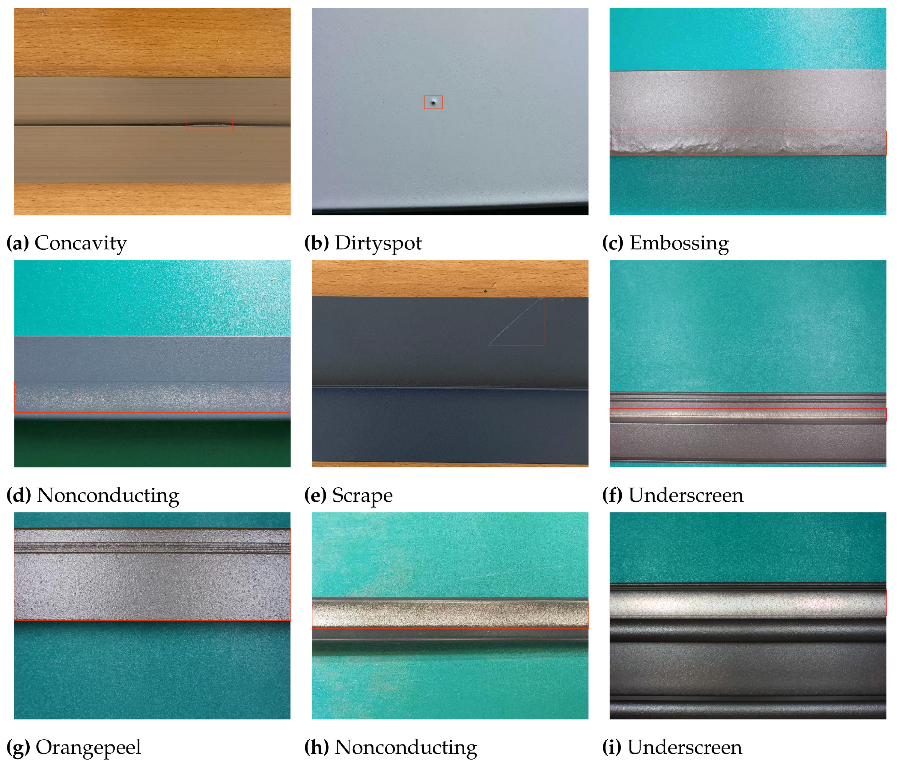
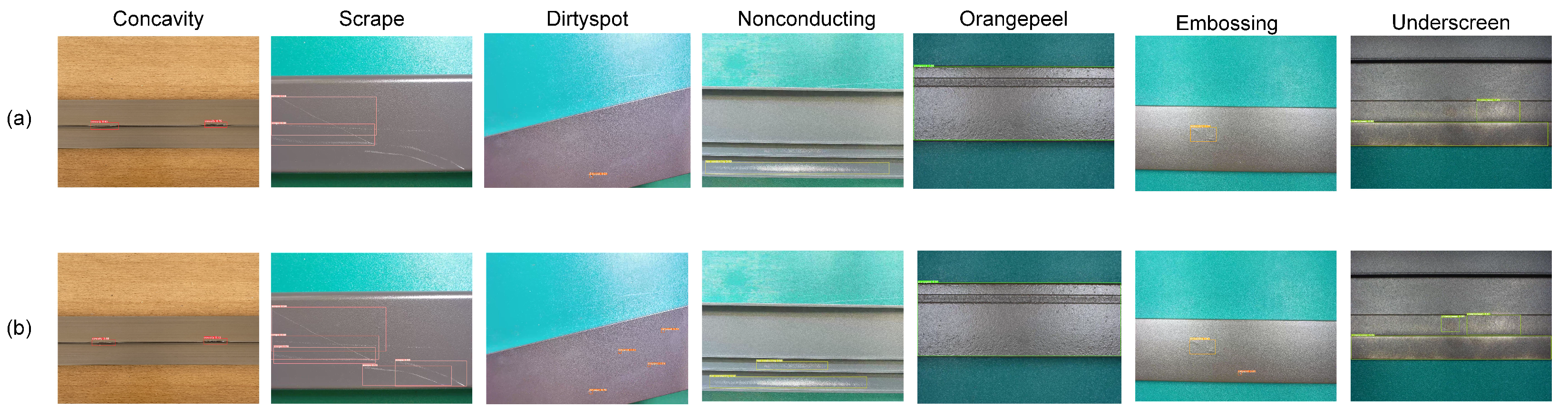
3.1. Aluminium Profile Defect Dataset
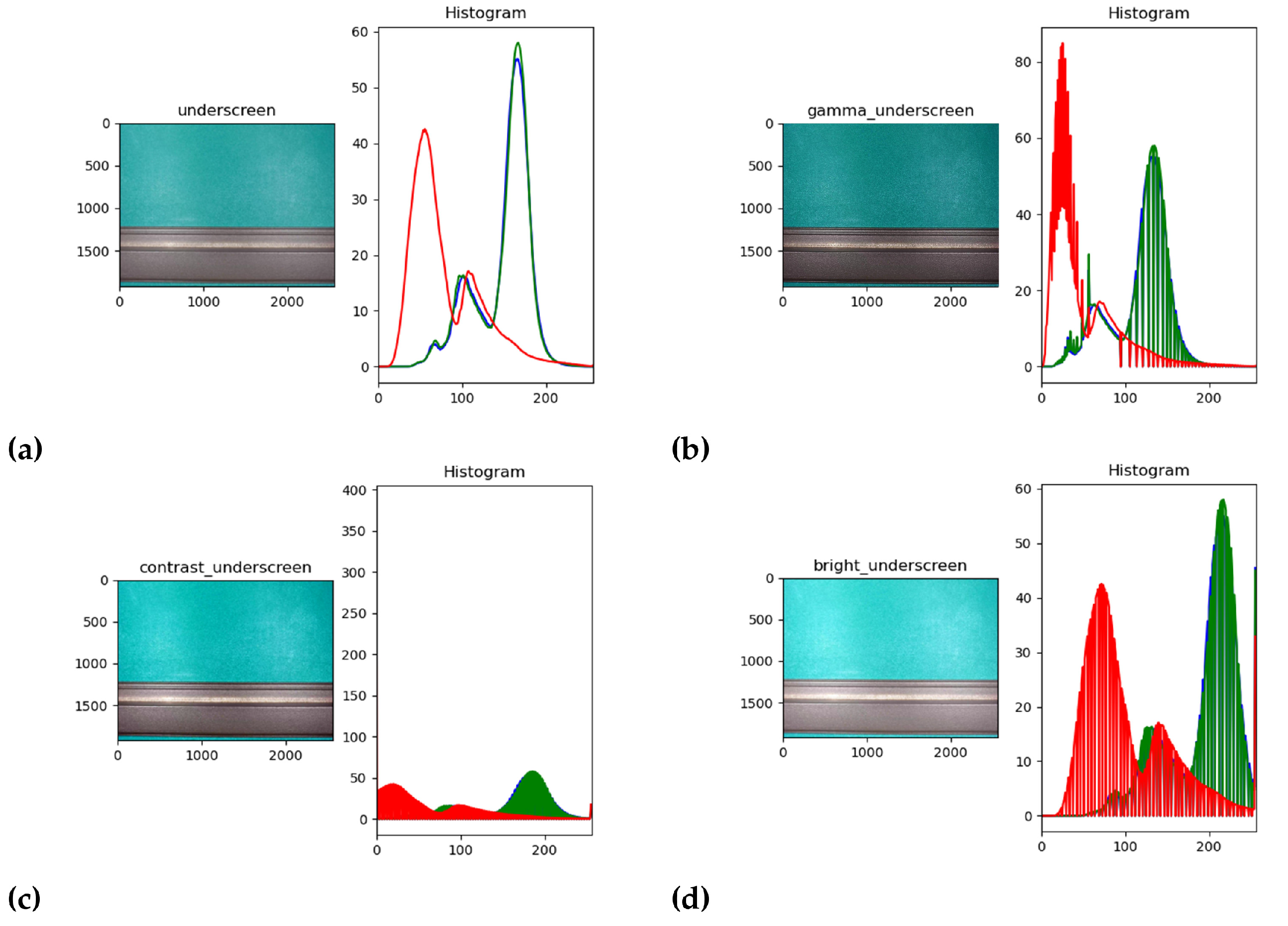
3.1.1. Gamma Variation
3.1.2. Contrast Variation and Brightness Variation
3.2. Methods
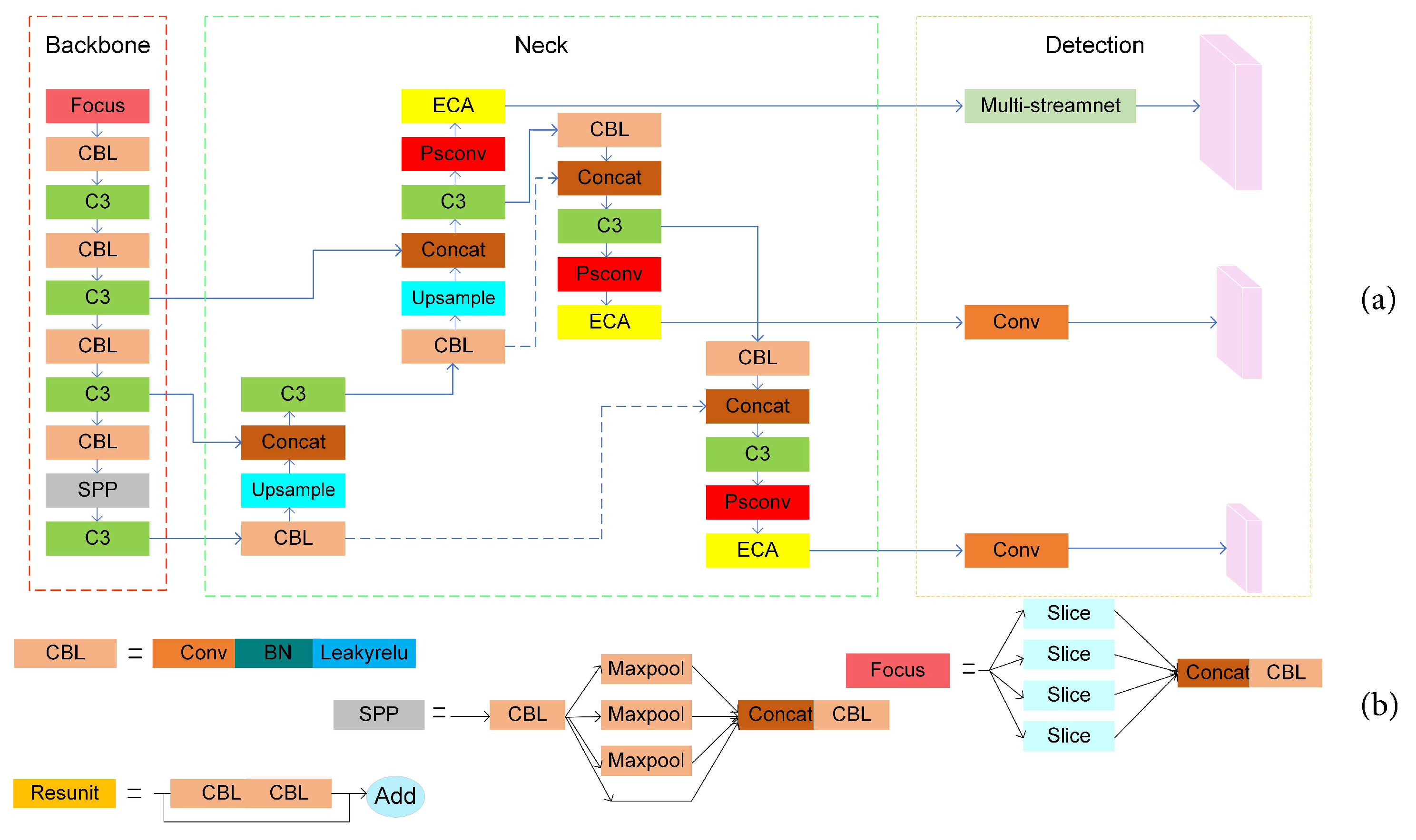
3.2.1. MS-YOLOv5
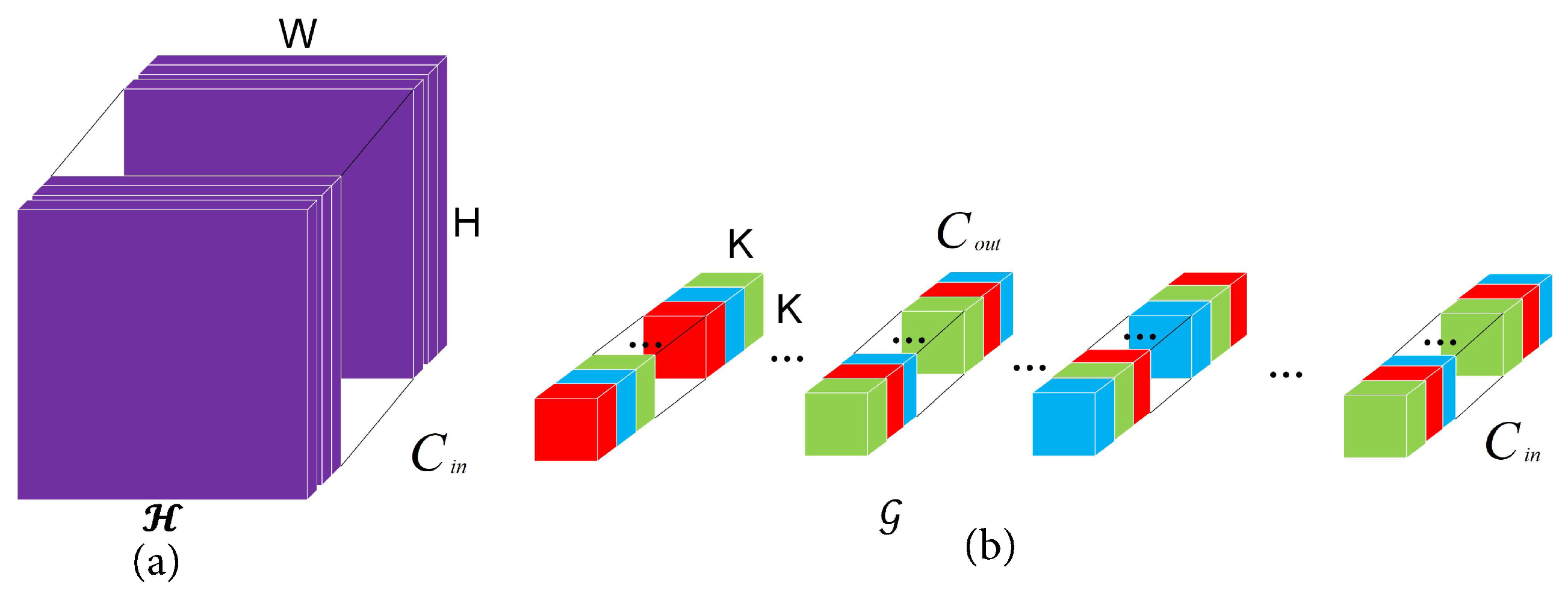
3.2.2. Poly-Scale Convolution
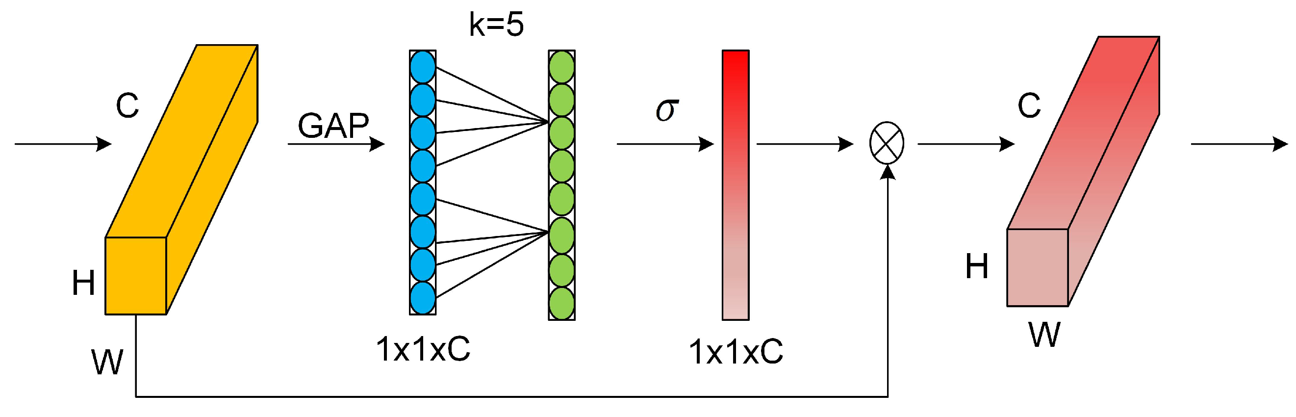
3.2.3. Efficient Channel Attention
3.2.4. PE-Neck
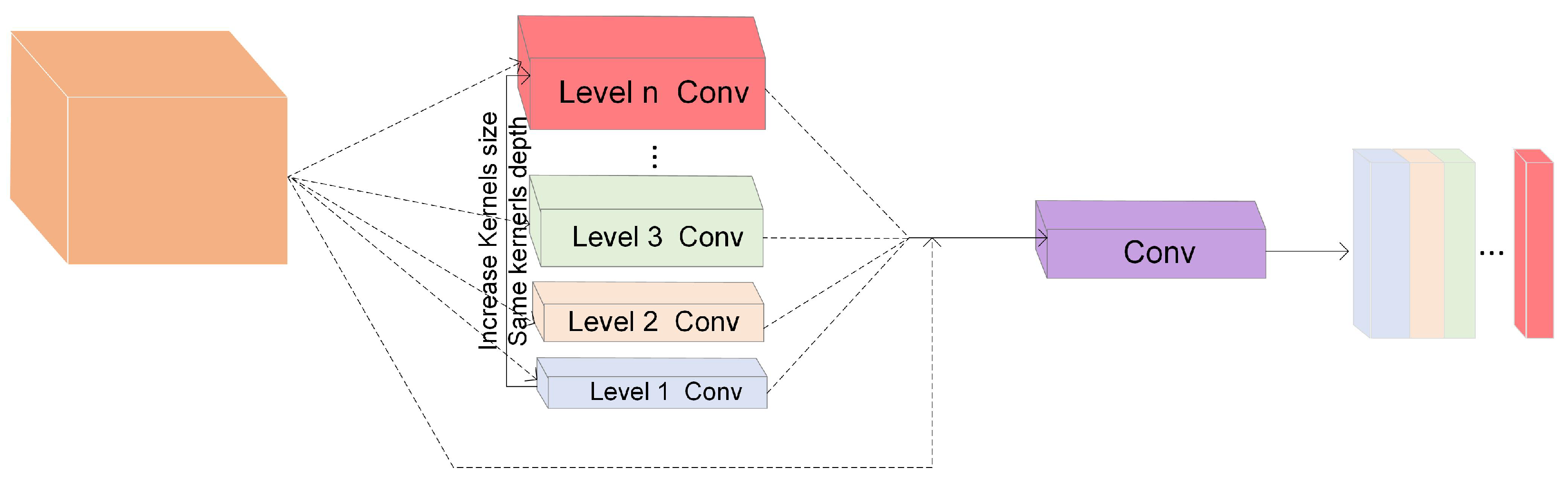
3.2.5. Multi-Streamnet
4. Experimental Environment, Evaluation Indicators, and Model Training
4.1. Experimental Environment
4.2. Experimental Evaluation Indicators
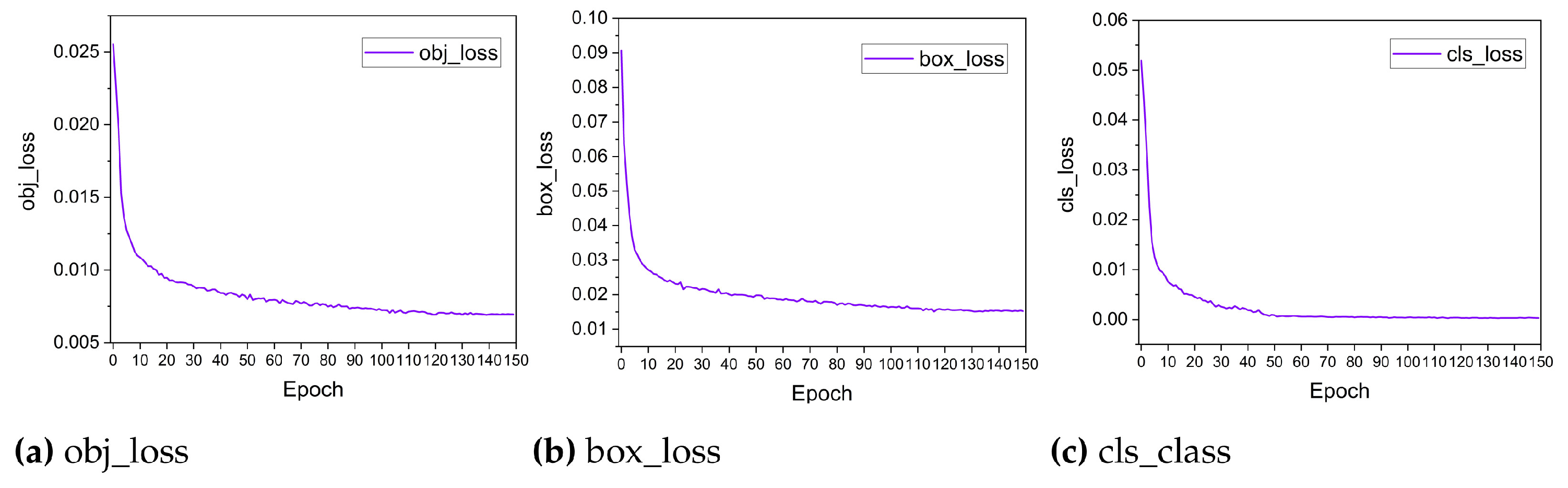
4.3. Model Training
5. Results
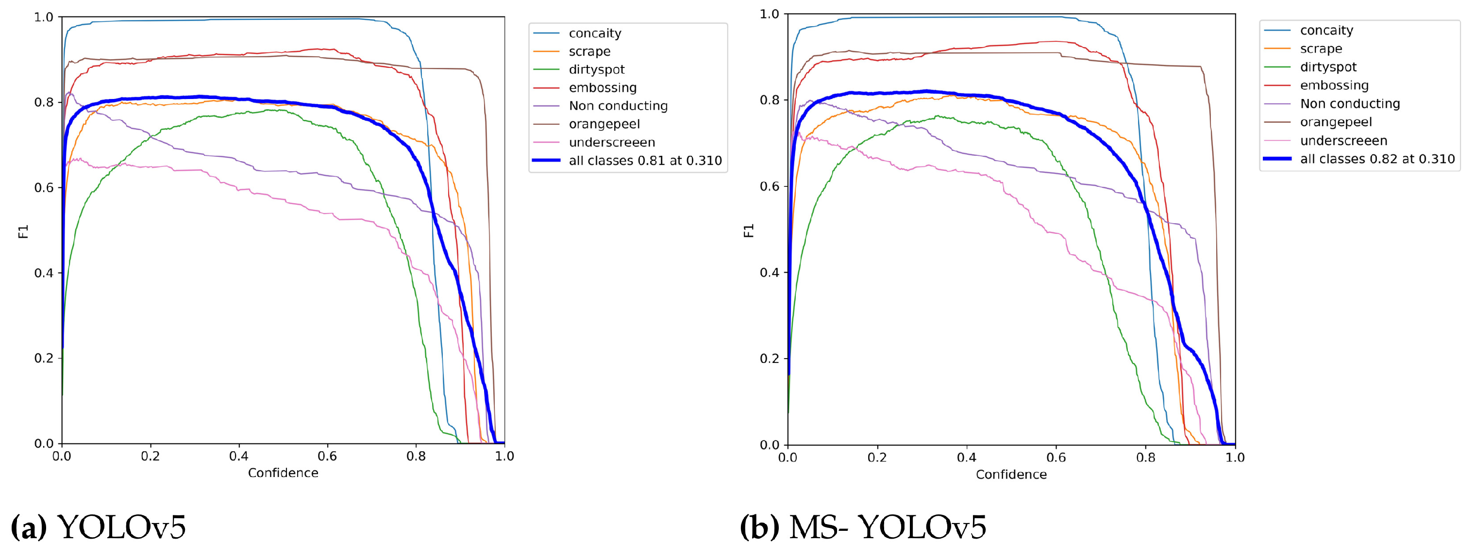
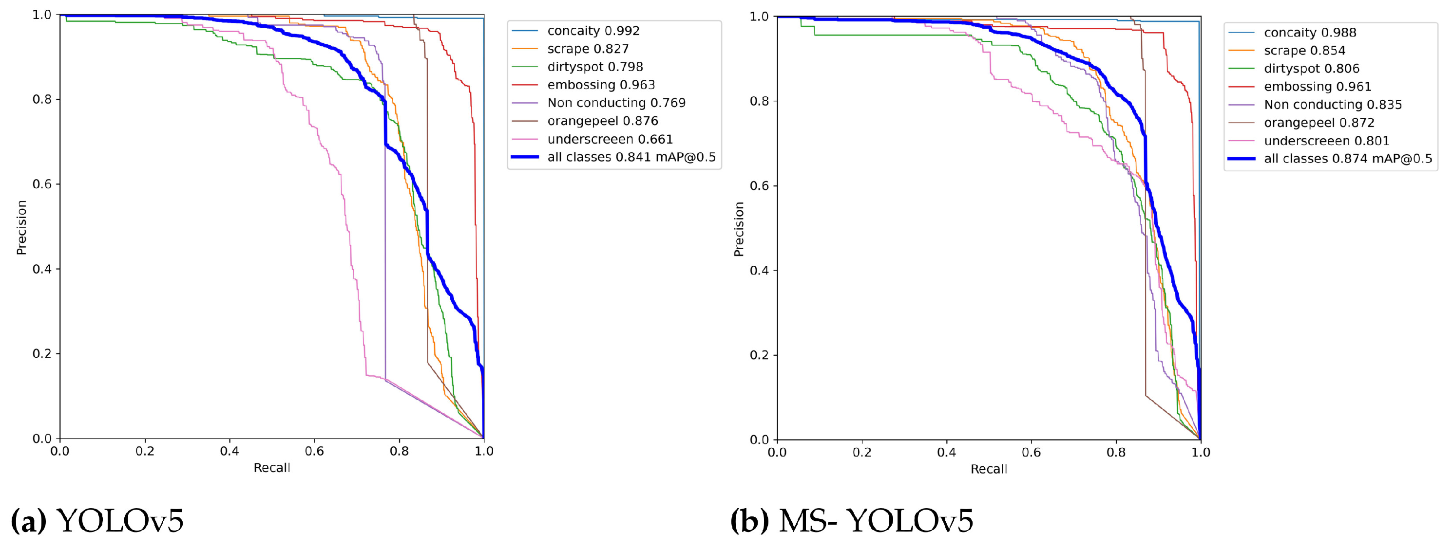
5.1. Validation of the MS-YOLOv5 Model
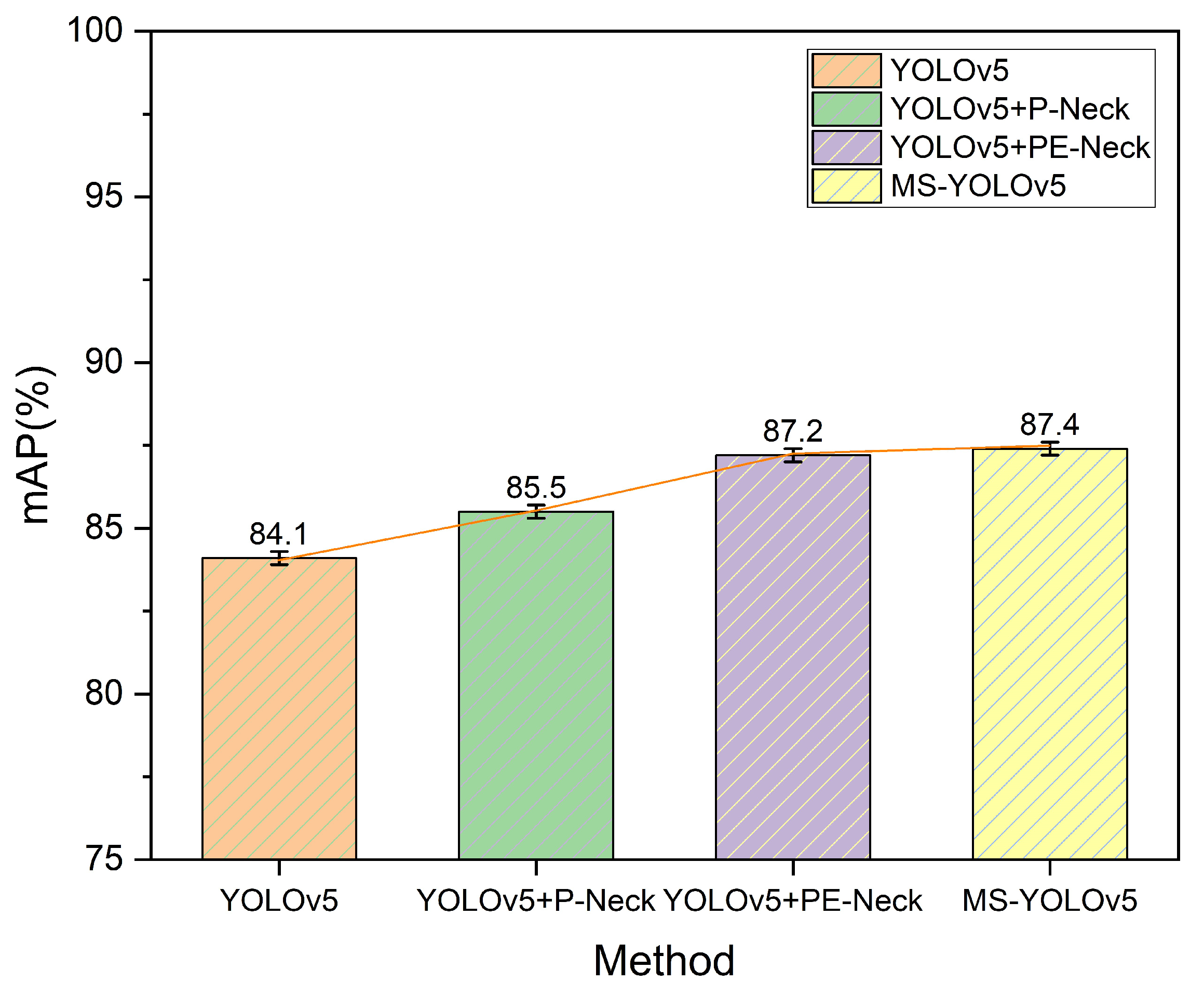
5.2. Ablation Comparison Experiments
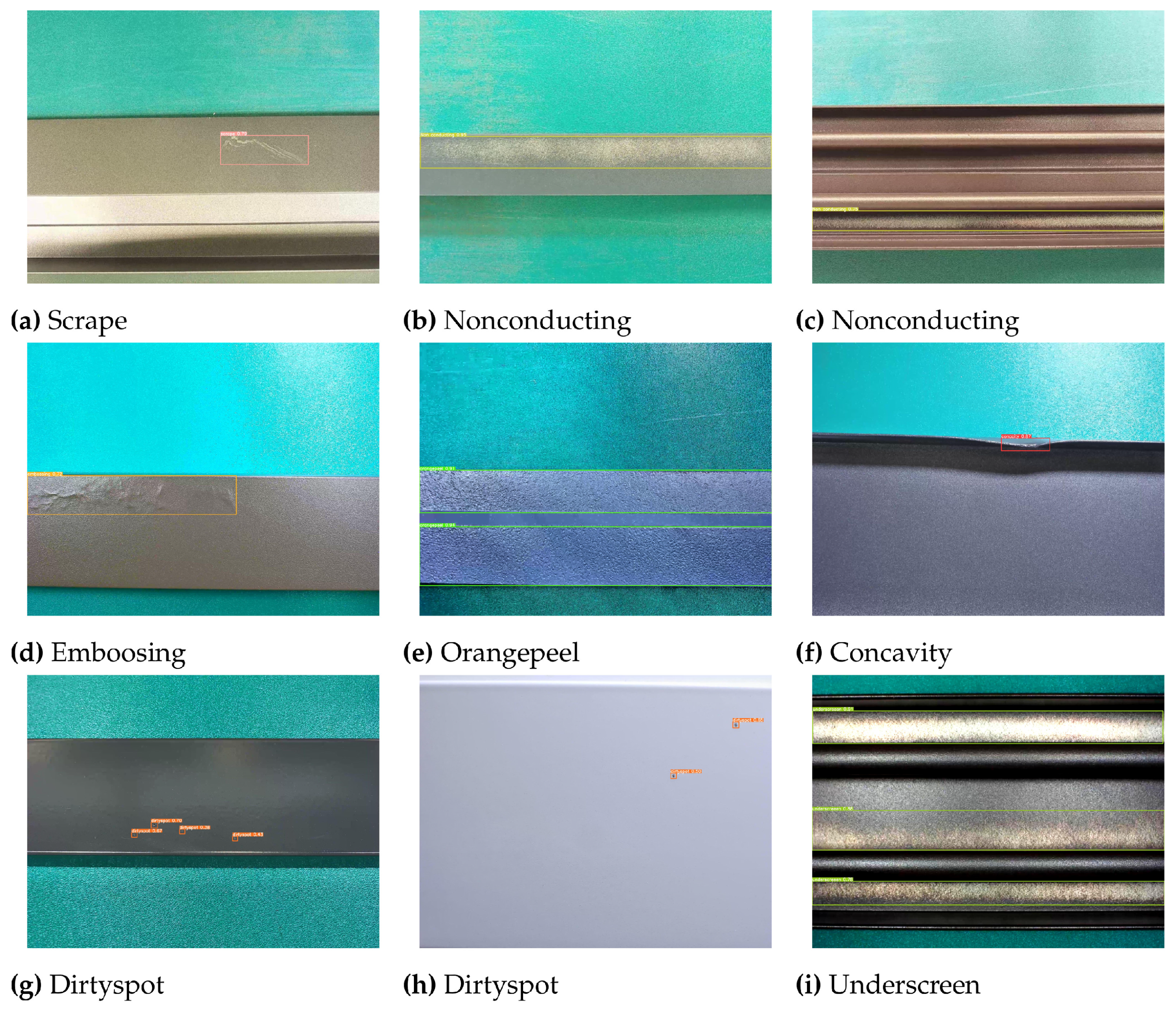
5.3. Experiments Comparing Different Algorithms
6. Conclusions
Author Contributions
Funding
Institutional Review Board Statement
Informed Consent Statement
Data Availability Statement
Conflicts of Interest
References
- Khatun, H.; Hazarika, S.; Sarma, U. Aluminium Plate Surface Defect Detection and CLassification based on Piezoelectric Transducers. In Proceedings of the 2021 IEEE 18th India Council International Conference (INDICON), Guwahati, India, 19–21 December 2021; IEEE: Piscataway, NJ, USA, 2021; pp. 1–6. [Google Scholar]
- Bustamante, L.; Jeyaprakash, N.; Yang, C.H. Hybrid laser and air-coupled ultrasonic defect detection of aluminium and CFRP plates by means of Lamb mode. Results Phys. 2020, 19, 103438. [Google Scholar] [CrossRef]
- Ramirez-Pacheco, E.; Espina-Hernandez, J.H.; Caleyo, F.; Hallen, J. Defect detection in aluminium with an eddy currents sensor. In Proceedings of the 2010 IEEE Electronics, Robotics and Automotive Mechanics Conference, Washington, DC, USA, 28 September 2010; IEEE: Piscataway, NJ, USA, 2010; pp. 765–770. [Google Scholar]
- Chen, P.H.; Lin, C.J.; Schölkopf, B. A tutorial on v-support vector machines. Appl. Stoch. Model. Bus. Ind. 2005, 21, 111–136. [Google Scholar] [CrossRef]
- Freund, Y.; Schapire, R.E. A decision-theoretic generalization of on-line learning and an application to boosting. J. Comput. Syst. Sci. 1997, 55, 119–139. [Google Scholar] [CrossRef] [Green Version]
- Rzepakowski, P.; Jaroszewicz, S. Decision trees for uplift modeling. In Proceedings of the 2010 IEEE International Conference on Data Mining, Sydney, Australia, 13 December 2010; IEEE: Piscataway, NJ, USA, 2010; pp. 441–450. [Google Scholar]
- Yan, K.; Dong, Q.; Sun, T.; Zhang, M.; Zhang, S. Weld defect detection based on completed local ternary patterns. In Proceedings of the International Conference on Video and Image Processing, Singapore, 27–29 December 2017; pp. 6–14. [Google Scholar]
- Aghdam, S.R.; Amid, E.; Imani, M.F. A fast method of steel surface defect detection using decision trees applied to LBP based features. In Proceedings of the 2012 7th IEEE Conference on Industrial Electronics and Applications (ICIEA), Singapore, 18–20 July 2012; IEEE: Piscataway, NJ, USA, 2012; pp. 1447–1452. [Google Scholar]
- Duan, F.; Yin, S.; Song, P.; Zhang, W.; Zhu, C.; Yokoi, H. Automatic welding defect detection of x-ray images by using cascade adaboost with penalty term. IEEE Access 2019, 7, 125929–125938. [Google Scholar] [CrossRef]
- Simonyan, K.; Zisserman, A. Very deep convolutional networks for large-scale image recognition. arXiv 2014, arXiv:1409.1556. [Google Scholar]
- Krizhevsky, A.; Sutskever, I.; Hinton, G.E. Imagenet classification with deep convolutional neural networks. Adv. Neural Inf. Process. Syst. 2012, 25. [Google Scholar] [CrossRef]
- He, K.; Zhang, X.; Ren, S.; Sun, J. Deep residual learning for image recognition. In Proceedings of the IEEE Conference on Computer Vision and Pattern Recognition, Las Vegas, NV, USA, 26 June–1 July 2016; pp. 770–778. [Google Scholar]
- Huang, G.; Liu, Z.; Van Der Maaten, L.; Weinberger, K.Q. Densely connected convolutional networks. In Proceedings of the IEEE Conference on Computer Vision and Pattern Recognition, Honolulu, HI, USA, 21–26 July 2017; pp. 4700–4708. [Google Scholar]
- Girshick, R.; Donahue, J.; Darrell, T.; Malik, J. Rich feature hierarchies for accurate object detection and semantic segmentation. In Proceedings of the IEEE Conference on Computer Vision and Pattern Recognition, Washington, DC, USA, 23–28 June 2014; pp. 580–587. [Google Scholar]
- Girshick, R. Fast r-cnn. In Proceedings of the IEEE International Conference on Computer Vision, Santiago, Chile, 7–13 December 2015; pp. 1440–1448. [Google Scholar]
- Faster, R. Towards real-time object detection with region proposal networks. Adv. Neural Inf. Process. Syst. 2015, 9199, 2969239–2969250. [Google Scholar]
- Redmon, J.; Divvala, S.; Girshick, R.; Farhadi, A. You only look once: Unified, real-time object detection. In Proceedings of the IEEE Conference on Computer Vision and Pattern Recognition, Las Vegas, NV, USA, 26 June–1 July 2016; pp. 779–788. [Google Scholar]
- Redmon, J.; Farhadi, A. YOLO9000: Better, faster, stronger. In Proceedings of the IEEE Conference on Computer Vision and Pattern Recognition, Honolulu, HI, USA, 21–26 July 2017; pp. 7263–7271. [Google Scholar]
- Redmon, J.; Farhadi, A. Yolov3: An incremental improvement. arXiv 2018, arXiv:1804.02767. [Google Scholar]
- Bochkovskiy, A.; Wang, C.Y.; Liao, H.Y.M. Yolov4: Optimal speed and accuracy of object detection. arXiv 2020, arXiv:2004.10934. [Google Scholar]
- Glenn Jocher, Alex Stoken, Jirka Borovec, NanoCode012. 2021. Available online: https://github.com/ultralytics/yolov5/ (accessed on 15 November 2021).
- Liu, W.; Anguelov, D.; Erhan, D.; Szegedy, C.; Reed, S.; Fu, C.Y.; Berg, A.C. Ssd: Single shot multibox detector. In Proceedings of the European Conference on Computer Vision, Amsterdam, The Netherlands, 8–16 October 2016; Springer: Berlin, Germany, 2016; pp. 21–37. [Google Scholar]
- Muresan, M.P.; Cireap, D.G.; Giosan, I. Automatic vision inspection solution for the manufacturing process of automotive components through plastic injection molding. In Proceedings of the 2020 IEEE 16th International Conference on Intelligent Computer Communication and Processing (ICCP), Cluj-Napoca, Romania, 3–5 September 2020; IEEE: Piscataway, NJ, USA, 2020; pp. 423–430. [Google Scholar]
- Usamentiaga, R.; Lema, D.G.; Pedrayes, O.D.; Daniel, G. Automated surface defect detection in metals: A comparative review of object detection and semantic segmentation using deep learning. IEEE Trans. Ind. Appl. 2022, 58, 4203–4213. [Google Scholar] [CrossRef]
- Schmitz, M. Machine Learning in Industrial Applications: Insights Gained from Selected Studies. Ph.D. Thesis, Friedrich-Alexander-Universität Erlangen-Nürnberg (FAU), Erlangen, Germnay, 2022. [Google Scholar]
- Gao, H.; Zhang, Y.; Lv, W.; Yin, J.; Qasim, T.; Wang, D. A Deep Convolutional Generative Adversarial Networks-Based Method for Defect Detection in Small Sample Industrial Parts Images. Appl. Sci. 2022, 12, 6569. [Google Scholar] [CrossRef]
- Jiang, Q.; Tan, D.; Li, Y.; Ji, S.; Cai, C.; Zheng, Q. Object detection and classification of metal polishing shaft surface defects based on convolutional neural network deep learning. Appl. Sci. 2019, 10, 87. [Google Scholar] [CrossRef] [Green Version]
- Di, H.; Ke, X.; Peng, Z.; Dongdong, Z. Surface defect classification of steels with a new semi-supervised learning method. Opt. Lasers Eng. 2019, 117, 40–48. [Google Scholar] [CrossRef]
- Xu, Y.; Zhang, K.; Wang, L. Metal Surface Defect Detection Using Modified YOLO. Algorithms 2021, 14, 257. [Google Scholar] [CrossRef]
- Wang, Y.; Hu, C.; Chen, K.; Yin, Z. Self-attention guided model for defect detection of aluminium alloy casting on X-ray image. Comput. Electr. Eng. 2020, 88, 106821. [Google Scholar] [CrossRef]
- Chen, S.; Wang, D.G.; Wang, F.B. Detecting aluminium tube surface defects by using faster region-based convolutional neural networks. J. Comput. Methods Sci. Eng. 2022; 1–10, Preprint. [Google Scholar]
- Tianchi Data Sets. Available online: https://tianchi.aliyun.com/dataset/ (accessed on 15 November 2021).
- Li, D.; Yao, A.; Chen, Q. Psconv: Squeezing feature pyramid into one compact poly-scale convolutional layer. In Proceedings of the European Conference on Computer Vision, Glasgow, UK, 23–28 August 2020; Springer: Berlin, Germany, 2020; pp. 615–632. [Google Scholar]
- Woo, S.; Park, J.; Lee, J.Y.; Kweon, I.S. Cbam: Convolutional block attention module. In Proceedings of the European Conference on Computer Vision (ECCV), Munich, Germany, 8–14 September 2018; pp. 3–19. [Google Scholar]
- Hu, J.; Shen, L.; Sun, G. Squeeze-and-excitation networks. In Proceedings of the IEEE Conference on Computer Vision and Pattern Recognition, Salt Lake City, UT, USA, 18–22 June 2018; pp. 7132–7141. [Google Scholar]
- Hou, Q.; Zhou, D.; Feng, J. Coordinate attention for efficient mobile network design. In Proceedings of the IEEE/CVF Conference on Computer Vision And Pattern Recognition, Nashville, TN, USA, 25 June 2021; pp. 13713–13722. [Google Scholar]
- Wang, Q.; Wu, B.; Zhu, P.; Li, P.; Hu, Q. ECA-Net: Efficient Channel Attention for Deep Convolutional Neural Networks. In Proceedings of the 2020 IEEE/CVF Conference on Computer Vision and Pattern Recognition (CVPR), Seattle, WA, USA, 13–19 June 2020. [Google Scholar]
- Duta, I.C.; Liu, L.; Zhu, F.; Shao, L. Pyramidal convolution: Rethinking convolutional neural networks for visual recognition. arXiv 2020, arXiv:2006.11538. [Google Scholar]
- Chen, Y.; Fan, H.; Xu, B.; Yan, Z.; Kalantidis, Y.; Rohrbach, M.; Yan, S.; Feng, J. Drop an octave: Reducing spatial redundancy in convolutional neural networks with octave convolution. In Proceedings of the IEEE/CVF International Conference on Computer Vision, Seoul, Korea, 27 October–2 November 2019; pp. 3435–3444. [Google Scholar]
- Gao, S.H.; Cheng, M.M.; Zhao, K.; Zhang, X.Y.; Yang, M.H.; Torr, P. Res2net: A new multi-scale backbone architecture. IEEE Trans. Pattern Anal. Mach. Intell. 2019, 43, 652–662. [Google Scholar] [CrossRef] [PubMed] [Green Version]
- Li, Y.; Kuang, Z.; Chen, Y.; Zhang, W. Data-driven neuron allocation for scale aggregation networks. In Proceedings of the IEEE/CVF Conference on Computer Vision and Pattern Recognition, Long Beach, CA, USA, 15–20 June 2019; pp. 11526–11534. [Google Scholar]


| Concacity | Dirtyspot | Scrape | Embossing | Underscreen | Nonconducting | Orangepeel | |
|---|---|---|---|---|---|---|---|
| Train | |||||||
| Original | 185 | 143 | 158 | 135 | 178 | 185 | 127 |
| H_flip | 185 | 143 | 158 | 135 | 178 | 185 | 127 |
| V_flip | 185 | 143 | 158 | 135 | 178 | 185 | 127 |
| HV_flip | 185 | 143 | 158 | 135 | 178 | 185 | 127 |
| Gamma | 185 | 143 | 158 | 135 | 178 | 185 | 127 |
| Contrast | 185 | 143 | 158 | 135 | 178 | 185 | 127 |
| Bright | 185 | 143 | 158 | 135 | 178 | 185 | 127 |
| Total | 7777 | ||||||
| Test | |||||||
| Original | 320 | 256 | 216 | 320 | 277 | 278 | 320 |
| Total | 1987 | ||||||
| Method | Precision (%) | Recall (%) | mAP (%) | FPS |
|---|---|---|---|---|
| YOLOv5 | 91.6 | 75.4 | 84.1 | 20.1 |
| YOLOv5+P-Neck | 89.8 | 77.9 | 85.5 | 19.8 |
| YOLOv5+PE-Neck | 90 | 78.5 | 87.2 | 19.5 |
| YOLOv5 + PE-Neck + Multi-streamnet(MS-YOLOv5) | 91.2 | 76.5 | 87.4 | 19.1 |
| Method | Precision (%) | Recall (%) | mAP (%) | FPS |
|---|---|---|---|---|
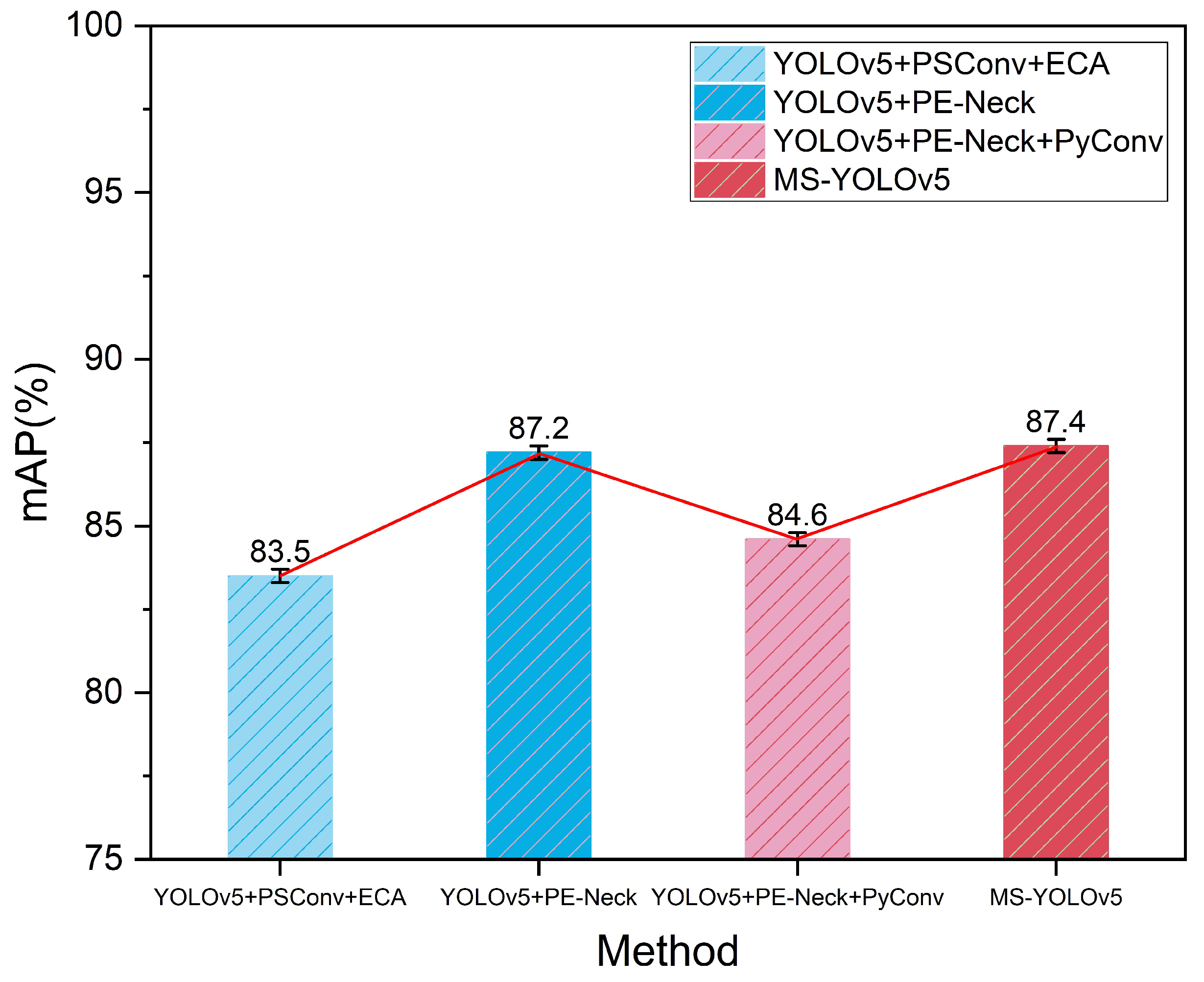
| YOLOv5+PSConv+ECA | 87.4 | 78 | 83.5 | 19.2 |
| YOLOv5+PE-Neck | 90 | 78.5 | 87.2 | 19.5 |
| YOLOv5+PE-Neck+PyConv | 89.4 | 77.7 | 84.6 | 18.4 |
| YOLOv5 + PE-Neck + Multi-streamnet(MS-YOLOv5) | 91.2 | 76.5 | 87.4 | 19.1 |
| Model | AP(%) | mAP(%) | FPS | ||||||
|---|---|---|---|---|---|---|---|---|---|
| Concavity | Scrape | Dirty Spot | Embossing | Non Conducting | Orange Peel | under Screen | |||
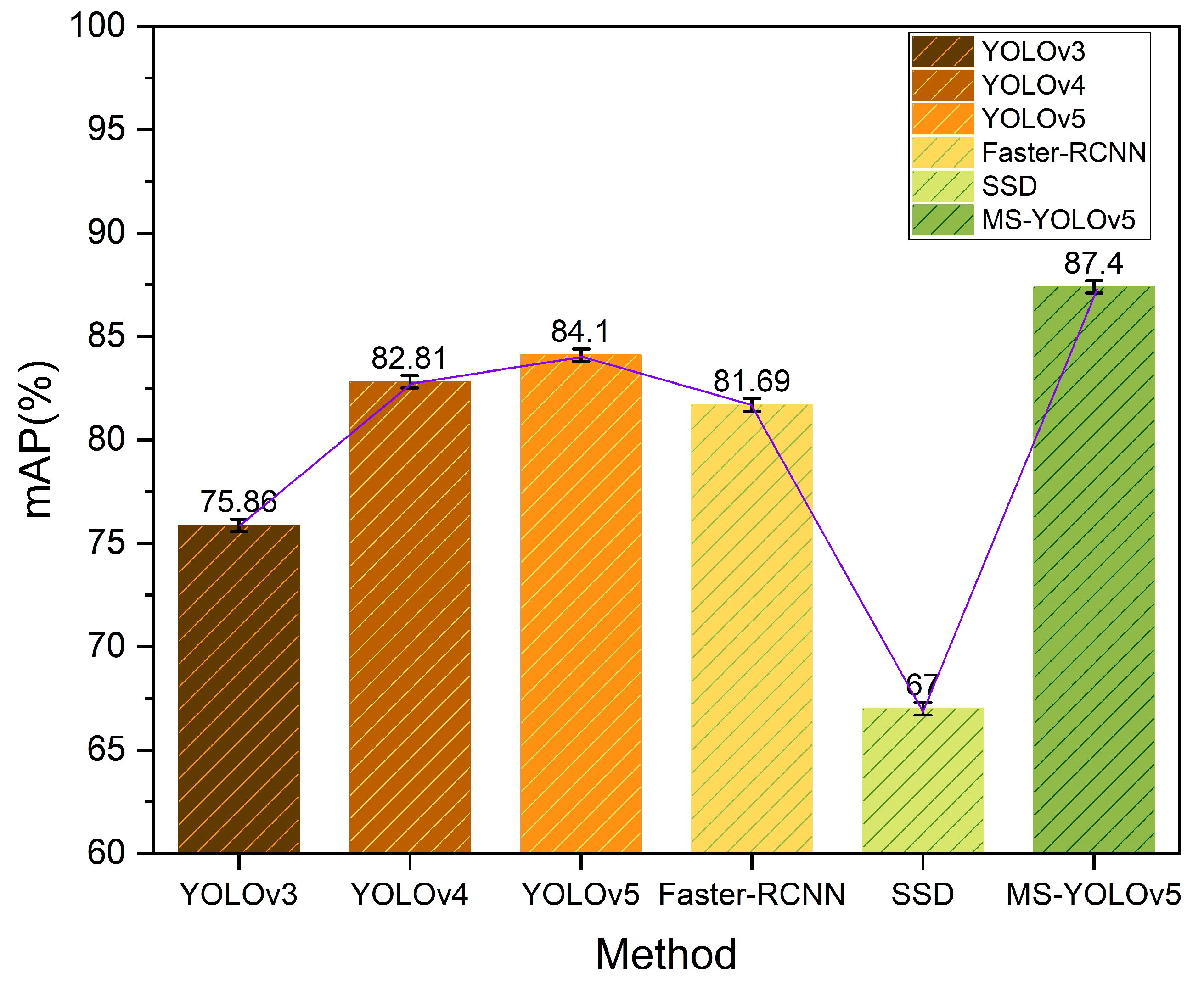
| YOLOv3 | 97.14 | 48.07 | 40.56 | 78.77 | 89.59 | 93.42 | 83.44 | 75.86 | 21.3 |
| YOLOv4 | 97.71 | 74.43 | 51.05 | 81.15 | 94.69 | 96.42 | 84.25 | 82.81 | 20.4 |
| YOLOv5 | 99.2 | 82.7 | 79.8 | 96.3 | 76.9 | 87.6 | 66.1 | 84.1 | 20.1 |
| SSD | 72.91 | 60.96 | 20.9 | 64.25 | 82.14 | 90.81 | 76.97 | 67 | 21.7 |
| Faster-RCNN | 92.14 | 70.74 | 38.7 | 94.03 | 90.36 | 97.40 | 88.49 | 81.69 | 12.6 |
| MS-YOLOv5 | 98.8 | 85.4 | 80.6 | 96.1 | 83.5 | 87.2 | 80.1 | 87.4 | 19.1 |
Publisher’s Note: MDPI stays neutral with regard to jurisdictional claims in published maps and institutional affiliations. |
© 2022 by the authors. Licensee MDPI, Basel, Switzerland. This article is an open access article distributed under the terms and conditions of the Creative Commons Attribution (CC BY) license (https://creativecommons.org/licenses/by/4.0/).
Share and Cite
Wang, T.; Su, J.; Xu, C.; Zhang, Y. An Intelligent Method for Detecting Surface Defects in Aluminium Profiles Based on the Improved YOLOv5 Algorithm. Electronics 2022, 11, 2304. https://doi.org/10.3390/electronics11152304
Wang T, Su J, Xu C, Zhang Y. An Intelligent Method for Detecting Surface Defects in Aluminium Profiles Based on the Improved YOLOv5 Algorithm. Electronics. 2022; 11(15):2304. https://doi.org/10.3390/electronics11152304
Chicago/Turabian StyleWang, Teng, Jianhuan Su, Chuan Xu, and Yinguang Zhang. 2022. "An Intelligent Method for Detecting Surface Defects in Aluminium Profiles Based on the Improved YOLOv5 Algorithm" Electronics 11, no. 15: 2304. https://doi.org/10.3390/electronics11152304