Article

Power-Efficient Trainable Neural Networks towards Accurate Measurement of Irregular Cavity Volume

1
School of Automobile and Traffic, Shenyang Ligong University, Shenyang 110159, China
2
School of Information Science and Engineering, Shenyang Ligong University, Shenyang 110159, China
3
School of Automation and Electrical Engineering, Shenyang Ligong University, Shenyang 110159, China
4
School of Equipment Engineering, Shenyang Ligong University, Shenyang 110159, China
*
Authors to whom correspondence should be addressed.
Electronics 2022, 11(13), 2073; https://doi.org/10.3390/electronics11132073
Submission received: 11 May 2022 / Revised: 20 June 2022 / Accepted: 23 June 2022 / Published: 1 July 2022
(This article belongs to the Special Issue Human Robot Interaction and Intelligent System Design)

Abstract

:
Irregular cavity volume measurement is a critical step in industrial production. This technology is used in a wide variety of applications. Traditional studies, such as waterflooding-based methods, have suffered from the following shortcomings, i.e., significant measurement error, low efficiency, complicated operation, and corrosion of devices. Recently, neural networks based on the air compression principle have been proposed to achieve irregular cavity volume measurement. However, the balance between data quality, network computation speed, convergence, and measurement accuracy is still underexplored. In this paper, we propose novel neural networks to achieve accurate measurement of irregular cavity volume. First, we propose a measurement method based on the air compression principle to analyze seven key parameters comprehensively. Moreover, we integrate the Hilbert–Schmidt independence criterion (HSIC) into fully connected neural networks (FCNNs) to build a trainable framework. This enables the proposed method to achieve power-efficient training. We evaluate the proposed neural network in the real world and compare it with typical procedures. The results show that the proposed method achieves the top performance for measurement accuracy and efficiency.

1. Introduction

Irregular cavities are one of the main parts produced by equipment manufacturing enterprises, and their volume is a key indicator of product production quality. Accurate and efficient measurement of the irregular cavity volume ensures various industrial production performance indicators and production quality [1]. However, it is difficult to use traditional methods to measure volume in many applications, such as in automobile engine combustion chambers, liquid storage tanks, supercharging devices, and vacuuming devices [2,3]. The traditional ways use the water injection process to measure irregular volume. These methods rely on hand-crafted techniques, which are labor intensive, have low measurement efficiency, and cause significant errors.

1.1. Related Work

Besides the traditional water-injection-based methods [4], the laser measurement method, orthogonal double-grating method [5], air pressure method [6], audio measurement method [7], and ultrasonic measurement method [8] have been reported by recent studies. These measurement methods have the following shortcomings: (1) complex hardware system, (2) high technical difficulty and low measurement efficiency, (3) significant error, and (4) complicated operation. These limitations hinder the volume measurement methods applied in the actual production. This paper provides new technologies for intelligent non-destructive measurements of the volume of irregular cavity components. The proposed technologies can significantly improve the volume measurement accuracy of irregular cavity components and alleviate the influence of human factors.
Recently, inspired by the success of the neural networks, many machine-learning--powered methods have been proposed for irregular volume measurement, such as in [9,10]. The neural network includes two processes, forward propagation and back propagation. Forward propagation aims to output the predicted value and the loss value [11]. In contrast, back propagation is based on the gradient descent algorithm and assigns the loss value to each neuron, changing each neuron’s corresponding weight, threshold, and loss [12]. However, in the real-world application of irregular volume measurement, the back-propagation techniques in most existing methods are very time-consuming and require a large amount of data. These methods with “garbage in” may face gradient disappearance and explosion problems. Furthermore, these methods explore learning rates and other hyperparameters based on the prior human experience [13,14].
More recent, how to balance training efficiency and measurement accuracy remains a challenge for most existing neural networks. This is because insufficient samples collected in the real world cannot meet the training requirements of the deep neural networks. The Hilbert–Schmidt independence criterion (HSIC) is proposed for training deep neural networks, and current studies have reported the extensions [15,16]. These methods show that the HSIC is comparable to cross-entropy-based back-propagation methods on popular classification datasets. These systems aim to make outputs different from classification labels. A single layer is used to train with SGD (without back propagation) to reformat the information, further improving the training efficiency of the model. HSIC-based methods successfully avoid the vanishing and exploding gradients of back propagation and achieve a fast convergence speed, strong generalization ability, and simple calculations [17].

1.2. Contributions

To solve the above problems, especially the challenges in real-world applications, we analyze the structural characteristics of irregular cavities and propose neural networks based on micro-compressed air for volume measurement. We design a corresponding measurement system and achieve the fast and accurate measurement of irregular cavity volume based on the proposed neural networks. We design the neural network based on fully connected neural networks (FCNNs), resulting in the advantages of a high training efficiency, low requirements for input data, and no restrictions. Powered by the FCNNs and the HSIC, the proposed method achieves leading performance in real-world volume measurement applications.
The main contributions of the paper are presented as follows:
(1)
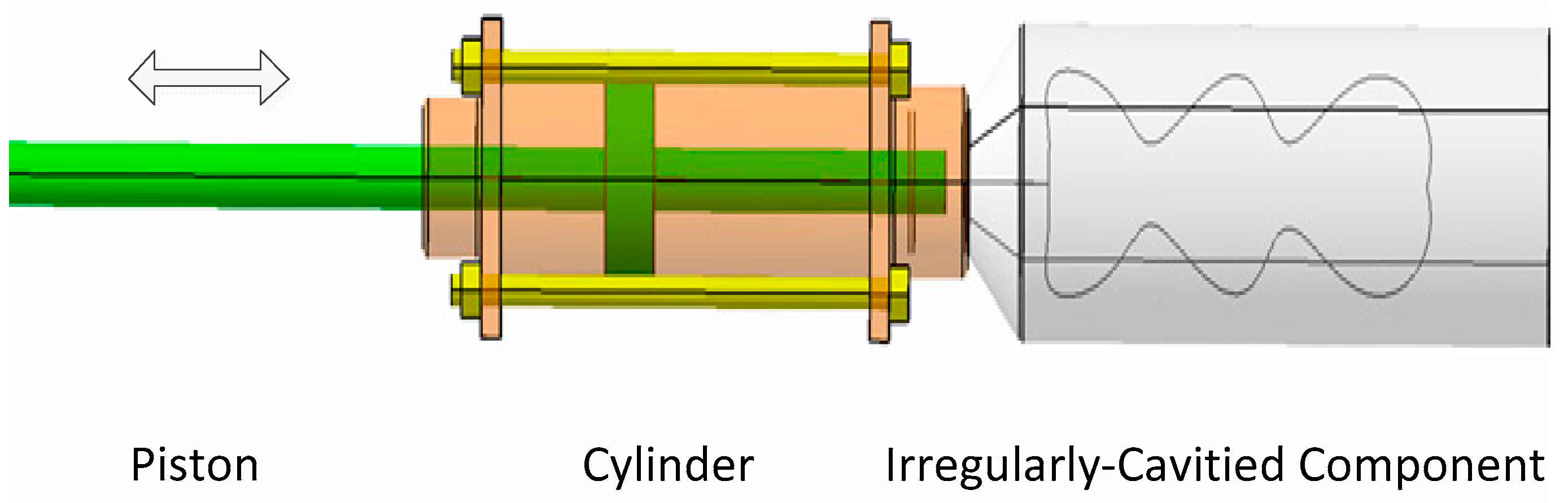
We design a micro-compressed air method to collect parameters related to the irregular cavity volume. To ensure that the read-to-measure parts are not damaged, the closed atmospheric air in the irregular cavity parts is slightly compressed, and the measurement parameters are collected.
(2)
We propose a method to analyze the main controlling factors affecting the volume detection of irregular cavity parts. We screen seven main characteristic parameters: pressure, temperature, humidity, gas equilibration time, etc. We carried out linear and nonlinear correlation analysis, feature selection, and normalization processing for the characteristic parameters. On this basis, we establish an irregular cavity volume measurement model based on FCNNs and the HSIC.
(3)
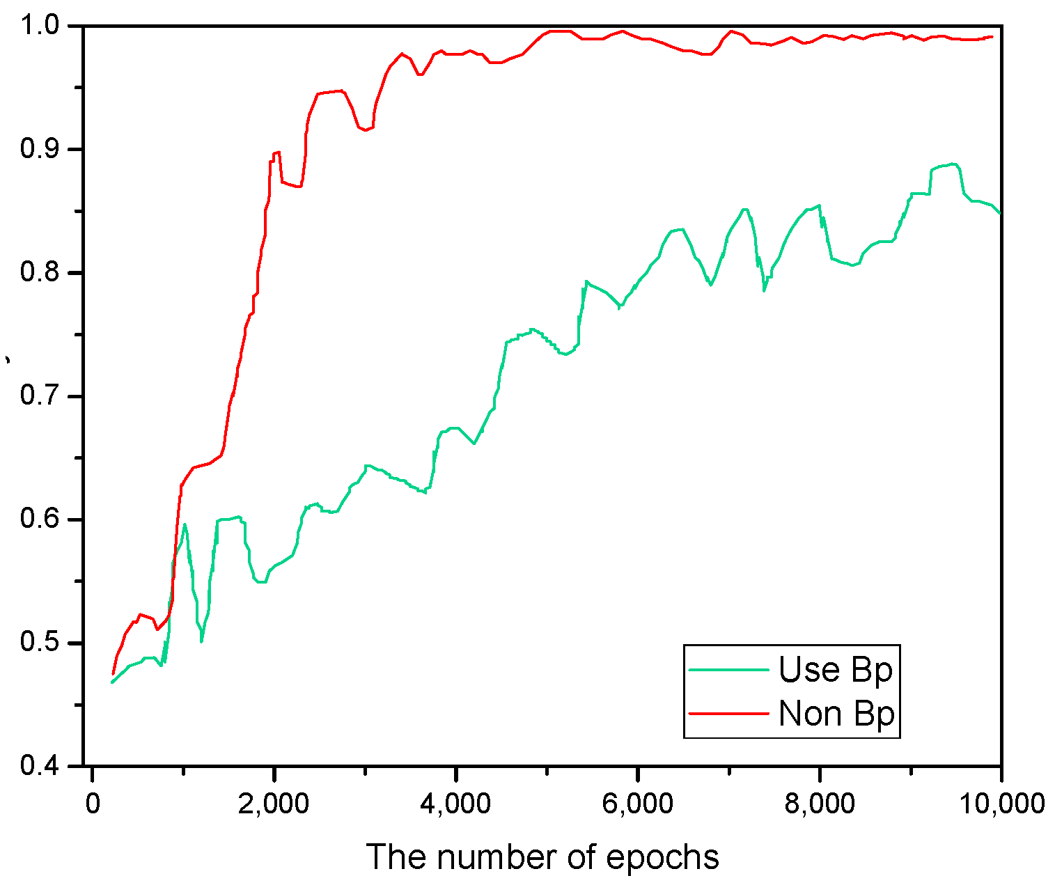
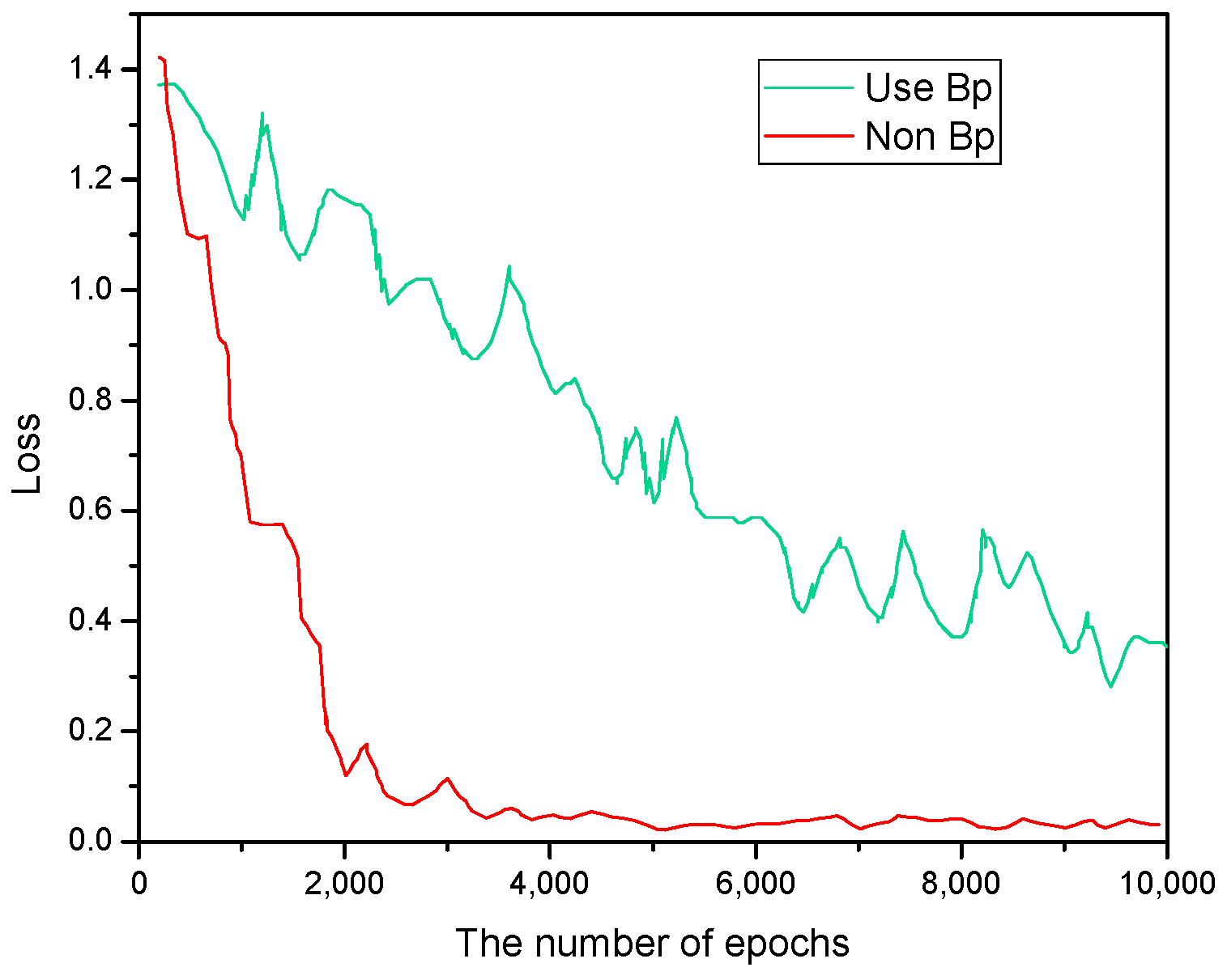
During the training process, we propose a new training scheme based on the HSIC. This method solves the challenges existing in the traditional BP-based methods. This method can reduce the error as much as possible and make the predicted value closer to the ground truth.
(4)
We conduct extensive experiments to evaluate the proposed neural network. We build a dataset for irregular volume measurement. The samples are collected in real-world applications. The results show the effectiveness and outperformance of the proposed method.
The paper is organized as follows. Section 2 presents a volume measurement method based on the micro-compressed air. Section 3 details the technology of the proposed neural network. Section 4 presents the experimental results and discussion. Section 5 concludes the paper and gives future study directions.

2. Preliminary

According to the ideal gas equation of state [18], the mass of the gas is conserved when the gas of a fixed group is in equilibrium. Its pressure, volume, and temperature have the following relationship:
PV = ZmRT
where P is the pressure of the gas (Pa), V is the volume of the gas (mL), Z is the compression coefficient of the gas (dimension is 1), m is the mass of the gas (mol), T is the temperature of the gas (K), and R is the gas constant (R =8.31 J/(mol·K)).
The detection principle is shown in Figure 1.
Experimental process:
(1)
Under the environment of normal temperature and pressure, the parts of the irregular cavity to be tested are filled with air of normal pressure;
(2)
Seal the air in the irregular cavity components to be tested. Record the ambient atmospheric pressure   P 1 , the stable differential pressure   P 2 of the gas in the cavity of the component to be tested, and the temperature   T 2 ;
(3)
The precision piston is controlled to extend completely into the cavity of the part to be tested, and the gas is slightly compressed. The volume of the piston completely entering the irregular cavity part to be tested is recorded as   V 0 ;
(4)
After thermodynamic equilibrium is achieved, experimental data are recorded including the ambient atmospheric pressure   P 1 , the stable differential pressure   P 2 of the gas in the parts, and the temperature   T 1 ;
As shown in Figure 1, under normal pressure, the air inside the irregular cavity is referred to as   V x , the pressure is   ( P 2 +   P 1 ) , and the temperature is T1. After micro-compressing the seal and setting the volume V0, the air volume is   ( V x V 0 ) , the pressure is   ( P 2 + P 1 ) , and the temperature is   T 1 . The state equation after micro-compression is as follows:
( P 2 + P 1 ) V x T 1 = ( P 2 + P 1 ) ( V x V 0 ) T 1
where   V x is the volume of the irregular cavity part to be measured. It can be deduced from the above formula:
V x = ( P 2 + P 1 ) T 1 ( P 2 + P 1 ) T 1 ( P 2 + P 1 ) T 1 V 0
According to Equations (2) and (3), the volume of the component to be tested is directly related to the atmospheric pressure, and the pressure and temperature before and after the micro-compression of the air inside the component. In addition, Table 1 and Figure 2 illustrate that the volume is also related to the time it takes for the air in the component to reach equilibrium after being compressed.
Table 1 and Figure 2 show that the detection volume is closer to the actual value as the equilibration time becomes longer. However, the testing time should not be too long. If the test time is prolonged, the pressure of the gas in the irregular cavity components is easily affected by temperature changes. In addition, the gas temperature and pressure inside the container tend to increase with the temperature of the environment, which makes the data change constantly. Therefore, the equilibration time was taken as 30 s.
Experiments show that environmental factors such as humidity and atmospheric pressure also bring some deviations to the gas state equation, just like temperature. This has a specific influence on the accuracy and stability of cavity volume detection. There is a complex relationship between these parameters and the cavity volume of the component under test, which is a nonlinear problem. As shown in Table 2, this paper uses atmospheric pressure, humidity, and other characteristic indicators as the input characteristic parameters of the volume prediction model of irregular cavity components, according to the experimental results.

3. Method

A neural network is a mathematical or computational model that mimics the structure and function of biological nerves [19]. It is used to estimate or approximate a function. A fully connected neural network is one of the connection methods, including input, hidden, and output layers [20,21,22,23,24]. An FCNN has a solid nonlinear fitting ability and can approach reality with high fitting accuracy [25]. However, its gradient descent algorithm is time-consuming and memory-intensive due to the constant search for suitable hyperparameters. The training time is longer, and the generalization effect is poor. This paper used the HSIC algorithm to replace the gradient back-propagation algorithm of the neural network. Compared with the traditional gradient back-propagation algorithm, its convergence speed and accuracy were significantly improved, and it had a strong generalization ability. At the same time, the amount of computation and memory footprint was greatly reduced. Therefore, this paper proposes a volume prediction model for irregular cavity parts based on FCNN and HSIC algorithms.

3.1. Preprocessing of Feature Data for Volume Prediction of Irregular Cavity Parts

To improve the training efficiency and prediction accuracy of the network, it is necessary to normalize the original data. Predicted values were denormalized to compare experimental results. There are two main methods of data normalization: maximum value normalization and mean-variance normalization [26]. The calculation formula of the maximum value normalization is shown as follows:
x norm = x x min x max x min
The principle of maximum value normalization is that all data are mapped between 0–1, suitable for cases where the data distribution has apparent boundaries. It is susceptible to outliers, which contribute to the overall skewness of the data. The calculation formula of the mean-variance normalization is shown as follows:
x norm = x x mean σ
where σ is the standard deviation of all sample data. Mean-variance normalization methods can adjust the data to a distribution with a mean of 0 and a variance of 1. It is not easily affected by outliers and is suitable for situations where the data distribution has no apparent boundaries and there are outliers. In this study, the maximum-minimum processing method is chosen. Since the value of “0” in the traditional method tends to have a more significant impact on the results, this paper improved the normalization method of the maximum and minimum values. The original data of the irregular cavity component volume was preprocessed, and the model’s predicted value was reversely preprocessed. The calculation formula of the data preprocessing method is shown as follows:
x norm = ( 0.8 0.2 ) × ( x x min ) x max x min + 0.2  
The calculation formula of the reverse preprocessing method is shown as follows:
  x = ( x norm 0.2 ) × ( x max x min ) 0.8 0.2 + x min  
where x is the original data of the irregular cavity component volume, x norm is the normalized data of various types, and x max and x min are the maximum and minimum values of various features of the original data, respectively.

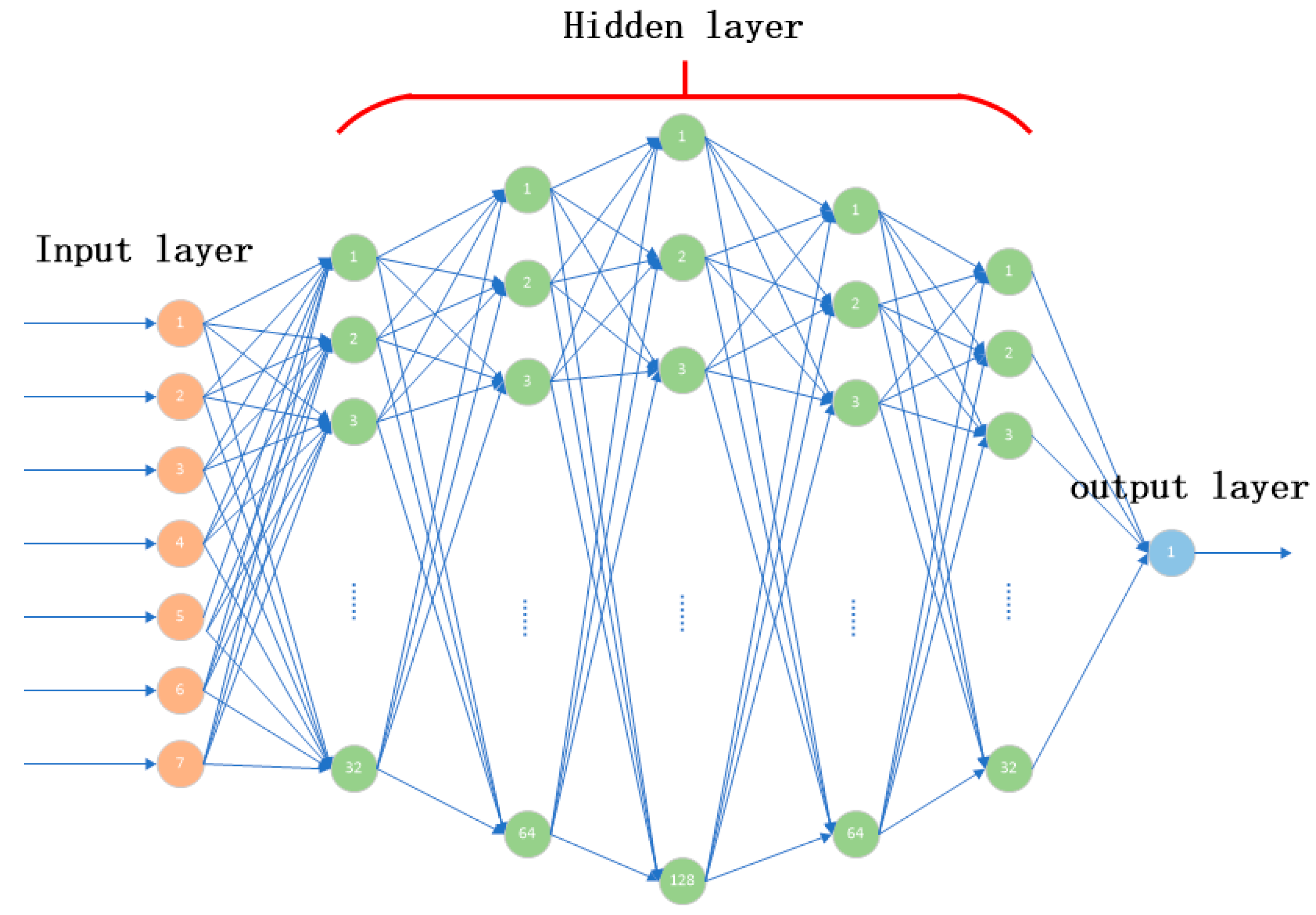
3.2. Establishment of the Volume Prediction Model of Irregular Cavity Components with Fully Connected Neural Network

Similar to the BP neural network structure, the FCNN performs a weighted summation of the input components and selects the corresponding activation function. Before constructing the volume prediction model, the basic parameters of the network are determined according to the characteristics of the network, such as activation function, number of neurons, number of network layers, learning rate, training step size, number of training times, and optimizer. The number of neurons has a significant impact on the learning and fitting capabilities of the model. Too few neurons and hidden layers make the model not capable enough to learn to mine the hidden features of the volume information of the parts. On the contrary, too many numbers make the model redundant, making it difficult to train or even overfit. Therefore, the basic parameters of the neural network need to be adapted to the research object.
Compared with the traditional neural network, the FCNN emphasizes the depth of the model. There are usually multiple hidden layers. This paper constructed a neural network with one input layer and one output layer, and its internal structure is shown in Figure 3. The selected 7 feature indicators helped determine the number of input neurons of the model to be 7 to match the preprocessed data. According to the Kolmogorov theorem and Hecht-Nielsen theory, the number of layers and nodes of the hidden layer is determined by the trial-and-error method. The final number of hidden layers was 5, and nodes were 32, 64, 128, 64, and 32. The model’s output is the predicted value of the volume of the irregular cavity components. The neurons in the output layer were set to 1, and the neural network topology was 7, 32, 64, 128, 64, 32, and 1.
The neural network training function adopts a gradient optimization method with an adaptive learning rate momentum factor. The activation function between the input and hidden layers is a sigmoid function, and the activation function between the hidden layer and output layer is a tanh function. The activation function between hidden layers is a leaky linear rectified unit (LeakyReLU) with a negative gradient. The initial model training step size was set to 10,000, and the amount of data (batch size) fed into the network for training was set to 32.
The mean absolute error (MAE) is used to test the gap between the model’s prediction and the actual value based on the loss function [27,28]. The mean absolute error (MAE) is the loss function generated by the running of the model, and the calculation formula is shown in Equation (8):
MAE = i = 1 n | y i y i p | n  
where y i and y i p are the actual volume value and the predicted value of the model, respectively, in milliliters, and n represents batch size.

3.3. HSIC Bottleneck Method

In this paper, the HSIC bottleneck method was adopted to replace the gradient backpropagation algorithm of the FCNN to avoid the problems of inefficiency and poor generalization of FCNNs [24]. The loss function has to be built to maximize the mutual information between the output and the label and minimize the mutual dependence between the input and output. In this way, the output can be predicted with the fewest input features, making the features of the hidden layer more efficient. This improved neural network training method is beneficial in preventing overfitting and improving generalization.
Traditional neural network training methods require using mutual information theory in the information bottleneck (IB). The IB principles encapsulate the concept of minimum sufficient statistics. It expresses the relationship between the information required for an optimally balanced prediction output and the information retained about the input. The optimal solution can be obtained by:
min p T i | X , p Y | T i I ( X ; O i ) β I ( O i ; Y )
where X and Y represent the input and label respectively, O i represents the output in the i th hidden layer, β represents the Lagrangian multiplier, I ( X ; O i ) represents the mutual information between X and O i , and I ( O i ; Y ) represents the mutual information between O i and Y . It can be seen from the formula that the IB mainly retains the output information of the labels in the hidden layer when compressing the input data features.
In practice, the IB is difficult to calculate due to a number of reasons. If the input signal is continuous, the mutual information I ( X ; O i ) is infinite unless a noise signal is added to the network. Therefore, many algorithms bin the input data, which does not expand the data to high dimensions. However, this will result in different results due to different binning rules. Additional influencing factors are the differences between discrete and continuous data, and between discrete data and differential entropy. This study uses the HSIC instead of mutual information, as in the IB principles. Unlike mutual information estimation, the HSIC adopts a robust calculation method for time complexity O ( l 2 ) , where l represents the number of input data.
The HSIC bottleneck is formed as follows. We introduce the cross-covariance operator in RKHS and defined HSIC as the Hilbert–Schmidt norm of the cross-covariance operator. Let x and y be two random variables, and extract samples ( x , y ) from the probability density functions of x and y . Define two nonlinear maps φ : X H , ψ : Y G . F and G represent the RKHS of x and y , respectively, and the corresponding kernel functions of x and y are:
k ( x ,   x ) = [ φ ( x ) , φ (   x ) ] , x ,   x X
l ( y ,   y ) = [ ψ ( y ) , ψ (   y ) ] , y ,   y Y
The cross-covariance operator C xy : G H for φ : X H and ψ : Y G is defined as:
C xy = E xy ( ( φ ( x ) μ x ) ( ψ ( y ) μ y ) )  
where represents the tensor product, and μ x = E x φ ( x ) , μ y = E y ψ ( y ) , and E x , E y , E xy represent mathematical expectations. HSIC is defined as the Hilbert–Schmidt norm squared:
HSIC ( P xy , H , G ) =   C xy HS 2 = E x   x   y   y ( k ( x ,   x ) l ( y ,   y ) ) + E x   x ( k ( x ,   x ) ) E y   y ( l ( y ,   y ) ) 2 E xy ( E   x ( k ( x ,   x ) ) E   y ( l ( y ,   y ) ) )    
where E x   x   y   y represents the joint mathematical expectation of ( x , y ) and (   x ,   y ) . For a pair of data Z = { ( x i , y i ) | i = 1 , , n } , the empirical estimate of HSIC is:
HSIC ( Z , H , G ) = 1 ( n 1 ) tr ( KHLH ) HSIC ( K , L )
where tr ( · ) represents the trace operation of the matrix, K , L R n × n represent the kernel matrix of K ij = k ( x i , x j ) and L ij = l ( y i , y j ) , respectively, H = I 1 n 11 T R n × n is the centering matrix, and 1 R n is the all-one vector.
In an FCNN composed of h hidden layers, the dimension of the output matrix is ( 1 , d i ) , where i { 1 , , h } , and d i represents the number of units in the i th hidden layer. The size of the hidden layer output matrix of each batch is ( b , d i ) , where b is the batch size. When applying IB principles to calculate the objective function, HSIC is used instead of mutual information:
Z i * = argmin Z i HSIC ( Z i , X ) β HSIC ( Z i , Y )
where M is the input data, N is the label data, and β is the Lagrangian multiplier. According to Equation (14), the terms of the HSIC in Equation (15) can be obtained as:
HSIC ( Z i , M ) = 1 ( n 1 ) tr ( K Z i HK M H )
HSIC ( Z i , N ) = 1 ( n 1 ) tr ( K Z i HK N H )
Equations (15)–(17) show that the optimal output Z_i finds a balance between redundant information independent of the input and maximum correlation with the output. Ideally, when Equation (14) converges, the information needed to predict the labels is preserved, eliminating redundant information that leads to overfitting.

4. Experiments

4.1. Experimental Settings

The project was built under TensorFlow and Keras frameworks. For fair comparison and comprehensive evaluation, we followed the popular experimental settings. First, we set the same parameters for the methods based on traditional BP training and non-BP training. Next, we tested the convergence speed and final prediction results under different learning rates. Finally, we compared the proposed model with state-of-the-art models using the same hyperparameter settings to analyze the performance.
This paper aimed to improve the performance of the proposed model in real-world applications. We designed a highly adaptable irregular cavity volume database by analyzing data types. We set the characteristic parameters that affect the volume of the irregular cavity to be measured as the training of the model, and the output variable is volume. In the real-world production process, we collected 2718 sets of samples, shuffled the order, and took 2000 sets as the training set, 360 sets as the validation set, and the remaining 358 sets as the test set.

4.2. Ablation Studies

To evaluate the contribution of the proposed different components to the system, we compared the results of different methods, including FCNN with HSIC, FCNN without HSIC, and SVM. According to the popular training setting, the Lagrangian multiplier of β in HSIC was set to 80.
Many ablation experiments are conducted under different parameter settings. We found the best scheme to integrate the non-BP algorithm into the proposed framework. The experiments set a batch size of 32 and a learning rate of 0.006. The proposed HSIC can train each layer individually, enabling individual optimization and parallel computation of each layer without passing forward gradients. To evaluate the proposed non-BP algorithm, we evaluated the accuracy and loss values of the proposed method and traditional BP training methods, as shown in Figure 4 and Figure 5.
Figure 4 shows that the traditional BP-based method did not reach convergence at 10,000 iterations, whereas the proposed method achieved convergence at 3000 iterations. The accuracy of the proposed method reached 0.9912, which is higher than that of the BP-based network. Figure 5 shows the variation of the loss function of the proposed method (MAE, red) and the traditional BP-based method (green) with the results of each iteration. It can be seen that the proposed algorithm achieved convergence at 3000 iterations and had higher accuracy. The proposed neural network performed better than traditional methods for irregular volume measurements.
During the training process, as the number of training steps increases, the MAE value output by the model drops sharply, and the change curves of the loss functions of the training set and the validation set are shown in Figure 6.
Figure 6 shows the results of the training set loss function (MAE, blue) and validation set loss function (red) of the fully connected neural network and HSIC model with each iteration. During the training process, the loss value kept decreasing as the training progressed, especially in the first 2500 iterations where the loss value decreased rapidly. Then, the decreasing trend slowed down significantly. At 3000 iterations, the model reached a convergence state, and the loss value was 0.135. Ultimately, the training and validation loss functions were almost equal, remaining stable at 5.0 × 10⁻³. The loss value showed a slow upward trend in the validation set at the 4300th iteration and finally stabilized after 5000 iterations. In addition, it can be seen that the model stops after 10,000 iterations, indicating that the comprehensive performance of the model is better.
As shown in Table 3 and Table 4, when the learning rate was 0.006, the value of MAE was the smallest, and when 6 layers of neural networks were selected, the amount of calculation and the value of MAE were the smallest.
Many nonlinear functions are used as activation functions in deep neural networks. We tested the performance using the elu, tanh, and relu functions as activation functions, as shown in Figure 7. It can be seen that the results were almost the same when using the tanh and the elu functions as activation functions. Although the accuracy curve was stable, the accuracy could not improve significantly as the number of iterations increased. The model was stuck in a local optimum, which was not as good as the results obtained with the ReLU function. When the ReLU function was used as the activation function, the accuracy curve was flat when it was stable, and the accuracy was significantly higher than the other two groups.
The learning rate directly affects how fast the model can converge to a local minimum (i.e., achieve the best accuracy). The larger the learning rate, the faster the neural network learns. The network may become stuck in a local optimum if the learning rate is too low. However, the loss stops falling beyond the extreme value and repeatedly oscillates at a specific position. We tested the training performance of the proposed algorithm at different learning rates, and the results are shown in Figure 8. The models converged at almost the same rate when the learning rates were 2.0 × 10⁻³ and 6.0 × 10⁻³. The model performed best when the learning rate was set to 6.0 × 10⁻³. The model converged significantly slower when the learning rate was set to 5.0 × 10⁴. Therefore, for better accuracy and latency, we determined the optimal learning rate to be 6.0 × 10⁻³.

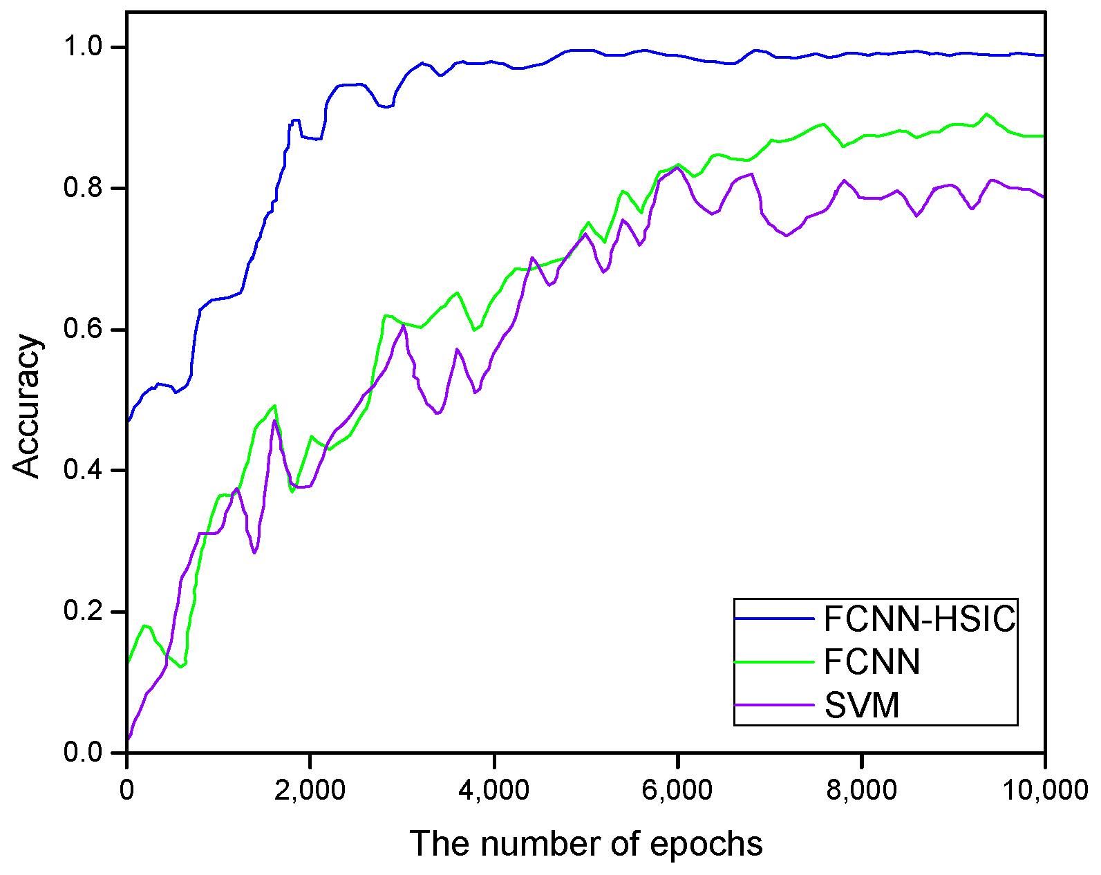
4.3. Comparison and Application

We compared the proposed method with the FCNN [29] and SVM [30] on the collected dataset. The learning rate was set to 6.0 × 10⁻³, and the batch size was 32, as shown in Figure 9. It is obvious that the proposed method converged faster than other methods. Compared with BP-based methods, the proposed method powered by the HSIC separated hidden signals in individual neuron representations, suggesting that the HSIC helps the distribution of extracted features achieve more independence and more accessible association with their labels.
The running time of the proposed techniques and the final results on the test set are shown in Table 5. The results show that the proposed model balanced accuracy and efficiency.

5. Conclusions

In this paper, to solve the challenges in the manual detection of irregular cavity volume measurements, i.e., manual detection is labor-intensive, low efficiency, and easy to corrode, we proposed neural networks for measuring irregular cavity volume based on micro-compressed air. A new dataset was established for the irregular cavity data collected in the production environment after data processing to improve the detection accuracy and reduce the influence of external environmental factors. The proposed method was motivated by FCNN and HSIC. After training, testing, and validation, we analyzed many experimental results. The experimental results show that the proposed method has a good effect on predicting irregular cavity volume, and the curve of accuracy and loss value is stable. The proposed model finally converged stably and achieved an accuracy of 0.9912 on the validation set. The proposed model has certain practicability and provides a new reference for studying irregular cavity volume measurement. The proposed method can achieve batch-to-batch consistency and product stability in industrial production. The results show that the proposed technologies have a good application prospect.
In a future study, we will introduce a feature fusion scheme to extract more discriminative features. This will enable the proposed system to reduce measurement errors. Next, we will design new loss functions to achieve a balance of fast convergence and improved accuracy.

Author Contributions

Conceptualization, H.G. and Y.J.; methodology, X.Z.; software, X.Z.; validation, W.Y., B.L. and Z.L.; formal analysis, X.Z.; investigation, X.Z.; resources, Y.J.; data curation, X.Z.; writing—original draft preparation, X.Z.; writing—review and editing, H.G.; visualization, X.Z.; supervision, Y.J.; project administration, Y.J.; funding acquisition, Y.J. All authors have read and agreed to the published version of the manuscript.

Funding

The authors would like to acknowledge support from the following projects: Liaoning Province Higher Education Innovative Talents Program Support Project (Grant No. XLYC1902095), Shenyang Young and Middle-aged Science and Technology Innovation Talent Support Program (Grant No. RC200386), LiaoNing Province Higher Education Innovative Talents Program Support Project (Grant No. LR2019058), LiaoNing Province Joint Open Fund for Key Scientific and Technological Innovation Bases (Grant No. 2021-KF-12-05), and Liaoning Province Basic Research Projects of Higher Education Institutions (Grant No. LG202107, LJKZ0239). the construction plan of scientific research and innovation team of Shenyang Ligong University (Grant No. SYLU202101), Comprehensive reform project of graduate education of Shenyang Ligong University (Grant No. 2021DSTD004, 2021PYPT006).

Institutional Review Board Statement

We exclude these statement because the study did not require ethical approval.

Informed Consent Statement

Not applicable.

Data Availability Statement

The data used to support the findings of this study are included within the article.

Conflicts of Interest

The authors declare no conflict of interest.

References

  1. Hao, G.U.; Jin-liang, F.E.; Yao-yu, Z.H.; Cun-liang, C.A.; Si-qi, L.I. High Precision Measurement of Cartridge Volume. Acta Armamentarii 2015, 36, 758. [Google Scholar]
  2. Strelnikova, E.; Gnitko, V.; Krutchenko, D.; Naumemko, Y. Free and forced vibrations of liquid storage tanks with baffles. Mod. Technol. Eng. 2018, 3, 15–52. [Google Scholar]
  3. Rogovyi, A. Energy performances of the vortex chamber supercharger. Energy 2018, 163, 52–60. [Google Scholar] [CrossRef]
  4. Sun, Y.; Xue, Z.; Hashimoto, T.; Zhang, Y. Optically quantifying spatiotemporal responses of water injection-induced strain via downhole distributed fiber optics sensing. Fuel 2021, 283, 118948. [Google Scholar] [CrossRef]
  5. Song, H.; Wang, Q.; Liu, M.; Cai, Q. A novel fiber Bragg grating vibration sensor based on orthogonal flexure hinge structure. IEEE Sens. J. 2020, 20, 5277–5285. [Google Scholar] [CrossRef]
  6. Bai, Y.; Zeng, J.; Huang, J.; Yan, Z.; Wu, Y.; Li, K.; Wu, Q.; Liang, D. Air pressure measurement of circular thin plate using optical fiber multimode interferometer. Measurement 2021, 182, 109784. [Google Scholar] [CrossRef]
  7. Cripe, J.; Aggarwal, N.; Lanza, R.; Libson, A.; Singh, R.; Heu, P.; Follman, D.; Cole, G.D.; Mavalvala, N.; Corbitt, T. Measurement of quantum back action in the audio band at room temperature. Nature 2019, 568, 364–367. [Google Scholar] [CrossRef]
  8. Cao, R.; Zhang, S.; Banthia, N.; Zhang, Y.; Zhang, Z. Interpreting the early-age reaction process of alkali-activated slag by using combined embedded ultrasonic measurement, thermal analysis, XRD, FTIR and SEM. Compos. Part B Eng. 2020, 186, 107840. [Google Scholar] [CrossRef]
  9. Sun, Y.; Yang, T.; Cheng, X.; Qin, Y. Volume measurement of moving irregular objects using linear laser and camera. In Proceedings of the 2018 IEEE 8th Annual International Conference on CYBER Technology in Automation, Control, and Intelligent Systems (CYBER), Tianjin, China, 19–23 July 2018; pp. 1288–1293. [Google Scholar]
  10. Kalantari, D.; Jafari, H.; Kaveh, M.; Szymanek, M.; Asghari, A.; Marczuk, A.; Khalife, E. Development of a machine vision system for the determination of some of the physical properties of very irregular small biomaterials. Int. Agrophys. 2022, 36, 27–35. [Google Scholar] [CrossRef]
  11. Arulmurugan, R.; Anandakumar, H. Early detection of lung cancer using wavelet feature descriptor and feed forward back propagation neural networks classifier. In Computational Vision and Bio Inspired Computing; Springer: Cham, Switzerland, 2018; pp. 103–110. [Google Scholar]
  12. Lyu, Z.; Yu, Y.; Samali, B.; Rashidi, M.; Mohammadi, M.; Nguyen, T.N.; Nguyen, A. Back-propagation neural network optimized by K-fold cross-validation for prediction of torsional strength of reinforced Concrete beam. Materials 2022, 15, 1477. [Google Scholar] [CrossRef]
  13. Wang, X.; An, S.; Xu, Y.; Hou, H.; Chen, F.; Yang, Y.; Zhang, S.; Liu, R. A back propagation neural network model optimized by mind evolutionary algorithm for estimating Cd, Cr, and Pb concentrations in soils using Vis-NIR diffuse reflectance spectroscopy. Appl. Sci. 2019, 10, 51. [Google Scholar] [CrossRef] [Green Version]
  14. Shaik, N.B.; Pedapati, S.R.; Taqvi, S.A.; Othman, A.R.; Dzubir, F.A. A feed-forward back propagation neural network approach to predict the life condition of crude oil pipeline. Processes 2020, 8, 661. [Google Scholar] [CrossRef]
  15. Jiang, H.; Tian, H.; Hua, Y.; Tang, B. Research on control of intelligent vehicle human-simulated steering system based on HSIC. Appl. Sci. 2019, 9, 905. [Google Scholar] [CrossRef] [Green Version]
  16. Ahmad, M.; Mazzara, M.; Distefano, S. Regularized cnn feature hierarchy for hyperspectral image classification. Remote Sens. 2021, 13, 2275. [Google Scholar] [CrossRef]
  17. Ma, W.D.; Lewis, J.P.; Kleijn, W.B. The HSIC bottleneck: Deep learning without back-propagation. In Proceedings of the AAAI Conference on Artificial Intelligence 2020, New York, NY, USA, 7–12 February 2020; Volume 34, pp. 5085–5092. [Google Scholar]
  18. Kuzevičová, Ž.; Gergeľová, M.; Kuzevič, Š.; Palková, J. Spatial interpolation and calculation of the volume an irregular solid. Int. J. Eng. 2014, 4, 8269. [Google Scholar]
  19. Ghimire, D.; Kil, D.; Kim, S.H. A Survey on Efficient Convolutional Neural Networks and Hardware Acceleration. Electronics 2022, 11, 945. [Google Scholar] [CrossRef]
  20. Wang, H.; Shi, H.; Lin, K.; Qin, C.; Zhao, L.; Huang, Y.; Liu, C. A high-precision arrhythmia classification method based on dual fully connected neural network. Biomed. Signal Process. Control 2020, 58, 101874. [Google Scholar] [CrossRef]
  21. Ganju, K.; Wang, Q.; Yang, W.; Gunter, C.A.; Borisov, N. Property inference attacks on fully connected neural networks using permutation invariant representations. In Proceedings of the 2018 ACM SIGSAC Conference on Computer and Communications Security, Toronto, ON, Canada, 15–19 October 2018; pp. 619–633. [Google Scholar]
  22. Aspri, M.; Tsagkatakis, G.; Tsakalides, P. Distributed Training and Inference of Deep Learning Models for Multi-Modal Land Cover Classification. Remote Sens. 2020, 12, 2670. [Google Scholar] [CrossRef]
  23. Aspri, M.; Tsagkatakis, G.; Panousopoulou, A.; Tsakalides, P. On Realizing Distributed Deep Neural Networks: An Astrophysics Case Study. In Proceedings of the 2019 27th European Signal Processing Conference (EUSIPCO), A Coruna, Spain, 2–6 September 2019; pp. 1–5. [Google Scholar]
  24. Tsagkatakis, G.; Aidini, A.; Fotiadou, K.; Giannopoulos, M.; Pentari, A.; Tsakalides, P. Survey of deep-learning approaches for remote sensing observation enhancement. Sensors 2019, 19, 3929. [Google Scholar] [CrossRef] [Green Version]
  25. Kobayashi, K.; Bolatkan, A.; Shiina, S.; Hamamoto, R. Fully-connected neural networks with reduced parameterization for predicting histological types of lung cancer from somatic mutations. Biomolecules 2020, 10, 1249. [Google Scholar] [CrossRef]
  26. Singh, D.; Singh, B. Investigating the impact of data normalization on classification performance. Appl. Soft Comput. 2020, 97, 105524. [Google Scholar] [CrossRef]
  27. Tomczyk, K.; Piekarczyk, M.; Sokal, G. Radial Basis Functions Intended to Determine the Upper Bound of Absolute Dynamic Error at the Output of Voltage-Mode Accelerometers. Sensors 2019, 19, 4154. [Google Scholar] [CrossRef] [PubMed] [Green Version]
  28. Tomczyk, K. Polynomial approximation of the maximum dynamic error generated by measurement systems. Prz. Elektrotech 2019, 95, 124–127. [Google Scholar] [CrossRef]
  29. Yuan, C.; Chen, J.; Chen, M.; Gu, W. A Lightweight CNN Using HSIC Fine-Tuning for Fingerprint Liveness Detection. In Proceedings of the Chinese Conference on Biometric Recognition 2021, Shanghai, China, 10–12 September 2021; Springer: Cham, Switzerland, 2021; pp. 240–247. [Google Scholar]
  30. Yue, J.; Xu, K.J.; Liu, W.; Zhang, J.G.; Fang, Z.Y.; Zhang, L.; Xu, H.R. SVM based measurement method and implementation of gas-liquid two-phase flow for CMF. Measurement 2019, 145, 160–171. [Google Scholar] [CrossRef]
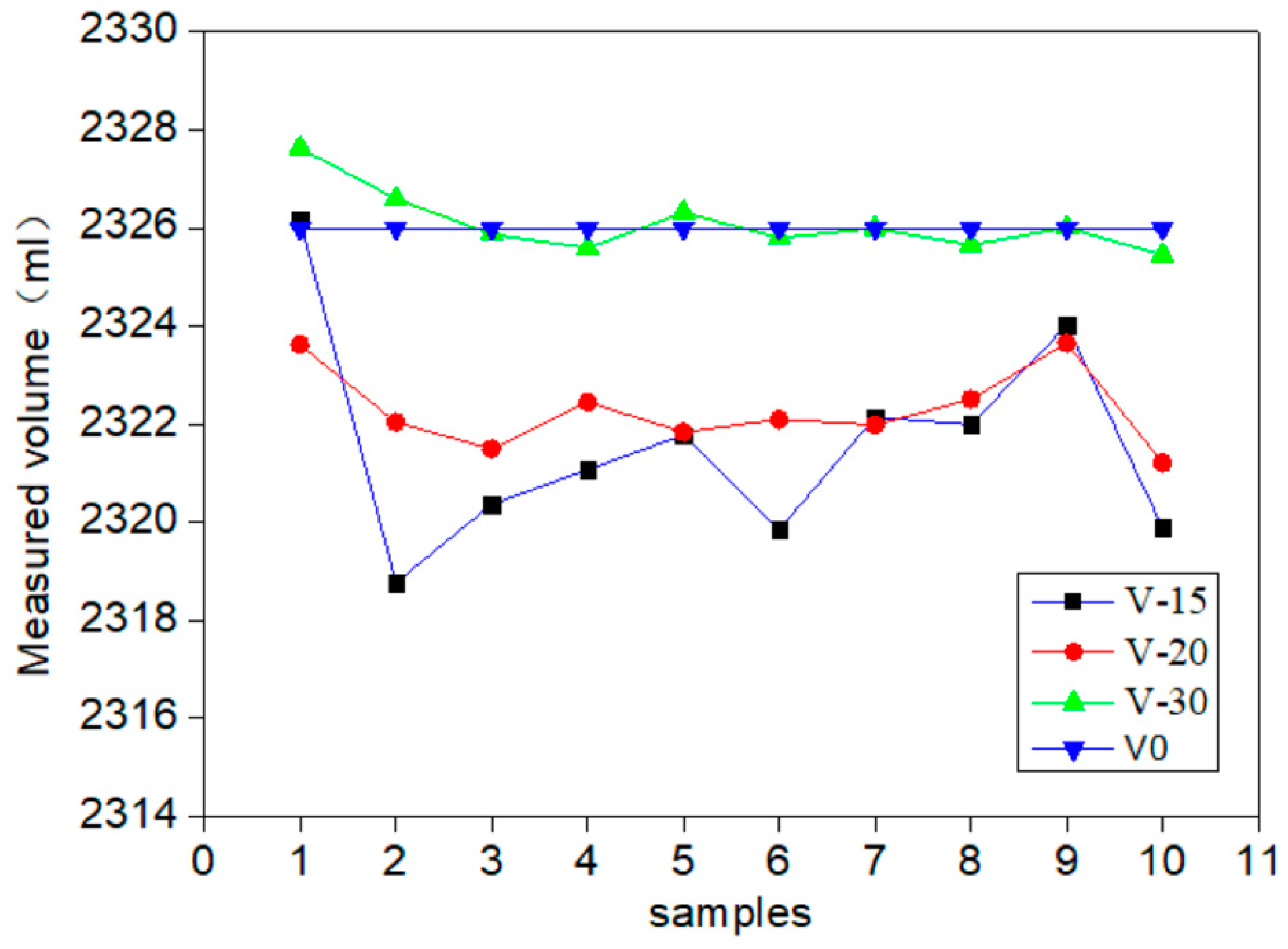
Figure 1. The volume detection principle schematic of irregular cavity components.
Electronics 11 02073 g001
Figure 2. The effect of gas equilibration time on detection.
Electronics 11 02073 g002
Figure 3. The volume prediction model structure of fully connected neural network.
Electronics 11 02073 g003
Figure 4. Accuracy curve: comparison of proposed non-BP and BP algorithm in the training process.
Electronics 11 02073 g004
Figure 5. Loss curve: comparison of proposed non-BP and BP algorithm in the training process.
Electronics 11 02073 g005
Figure 6. The loss curves of the training and validation sets.
Electronics 11 02073 g006
Figure 7. The accuracy curve of different activation functions.
Electronics 11 02073 g007
Figure 8. Accuracy under different learning rates.
Electronics 11 02073 g008
Figure 9. Accuracy of different models on the collected dataset.
Electronics 11 02073 g009
Table 1. Effect of gas equilibration time on volume detection, where V0 is the actual value of the volume, V-15 is the volume value detected when the gas equilibration time is 15 s, and V-20 and V-30 are also similar.
GroupV0
mL
V-15
mL
V-20
mL
V-30
mL
123262326.162323.622327.63
223262318.772322.042326.60
323262320.372321.492325.88
423262321.072322.452325.59
523262321.782321.842326.32
623262319.852322.102325.80
723262322.142321.982325.99
823262321.992322.512325.66
923262324.022323.652326.01
1023262319.892321.212325.45
Table 2. Input characteristic parameters of irregular cavity components.
NumberFeature Parameters
1Atmospheric pressure
2Atmospheric humidity
3Temperature before micro-compression
4Stable differential pressure before micro-compression
5Temperature after micro-compression
6Stable differential pressure after micro-compression
7Gas equilibration time
Table 3. Values of the MAE.
lr0.00050.0010.0020.0030.0040.0050.0060.0070.008
MAE0.0110.0100.0090.0070.0060.0060.0050.0060.006
Table 4. MAE under different settings.
LayersParametersMAE
440961.112
620,4800.005
886,0160.005
Table 5. Comparison of different methods on the collected dataset.
MethodPer Step CPU TimeAccuracy in Test Set
SVM0.326125 s0.76
FCNN0.576233 s0.85
Proposed0.176329 s0.99
Publisher’s Note: MDPI stays neutral with regard to jurisdictional claims in published maps and institutional affiliations.

