Pyramidal Predictive Network: A Model for Visual-Frame Prediction Based on Predictive Coding Theory

Abstract

Visual-frame prediction is a pixel-dense prediction task that infers future frames from past frames. A lack of appearance details, low prediction accuracy and a high computational overhead are still major problems associated with current models or methods. In this paper, we propose a novel neural network model inspired by the well-known predictive coding theory to deal with these problems. Predictive coding provides an interesting and reliable computational framework. We combined this approach with other theories, such as the theory that the cerebral cortex oscillates at different frequencies at different levels, to design an efficient and reliable predictive network model for visual-frame prediction. Specifically, the model is composed of a series of recurrent and convolutional units forming the top-down and bottom-up streams, respectively. The update frequency of neural units on each of the layers decreases with the increase in the network level, which means that neurons of a higher level can capture information in longer time dimensions. According to the experimental results, this model showed better compactness and comparable predictive performance with those of existing works, implying lower computational cost and higher prediction accuracy.

1. Introduction

The idea that brains are essentially prediction machines is one of the unified theories in cognitive science. It holds that brain functions, such as perception, motor control and memory, are all formed and modulated by prediction. Particularly, it also forms a sensorimotor framework (predictive coding) for understanding how a human takes an action based on predictions. It proposes that most functions in the brain follow a predictive framework, which is expressed by our brain’s internal model. Therefore, the brain can continuously predict and form our perceptions, on the basis of which we can also execute motor actions. Such an internal predictive model, shaped by the neurons’ representations, is also always learning and updating itself in order to predict the changing environment better. This idea, if it is properly implemented by learning architectures, could also be useful in practical applications such as video-frame prediction.

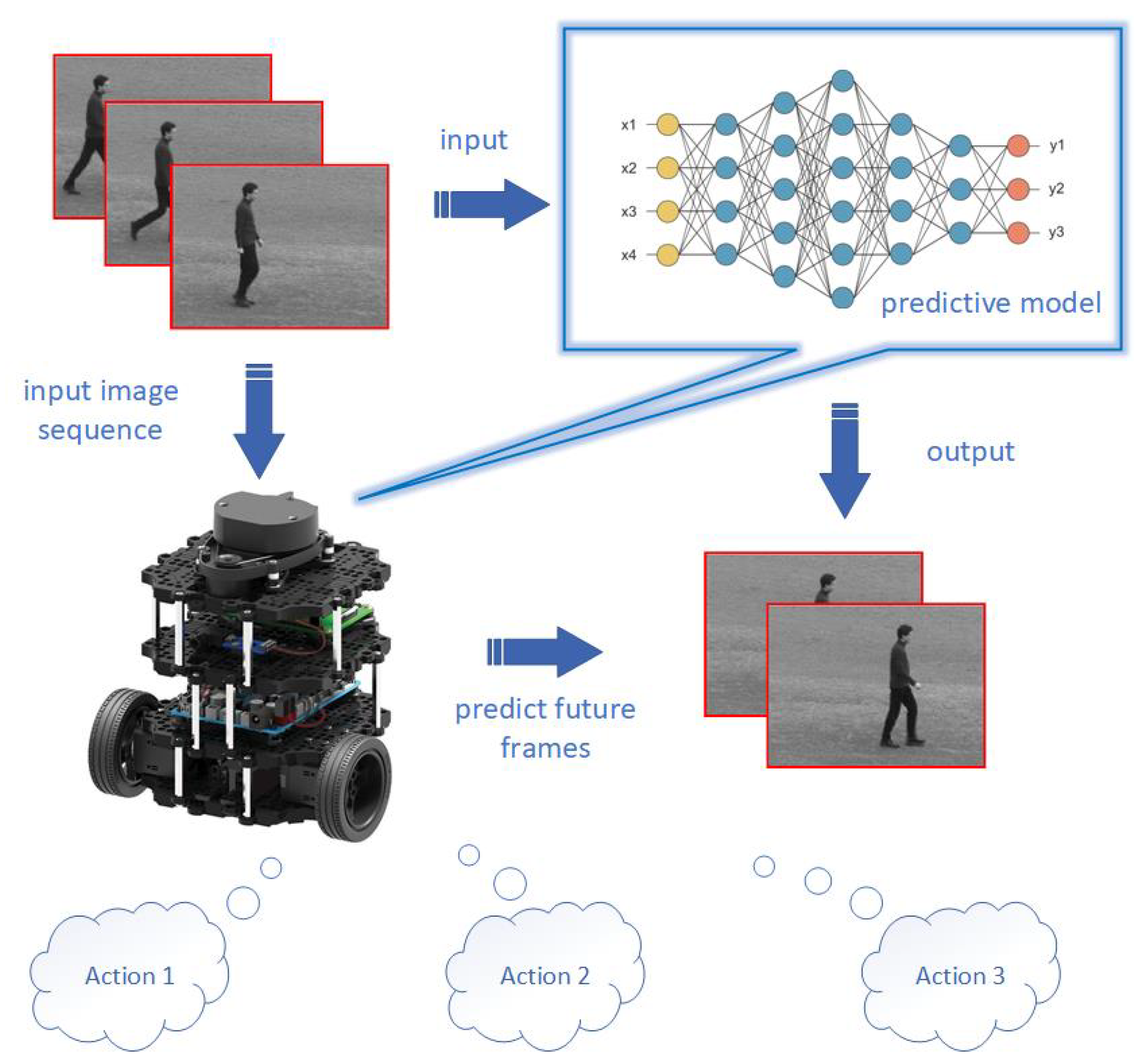
The so-called video-frame prediction task involves predicting the future of a visual frame based on the given contextual frames. From the perspective of applications, being able to predict the future is of great significance. Adaptive systems that can predict how future scenes may unfold based on an internal model that can learn from context will offer numerous possibilities.For example, a predictive ability would enable robots to foresee the future and even to understand humans’ intentions by analyzing their movements, actions, etc., to perform correct actions ahead of time (Figure 1). Self-driving cars can anticipate forthcoming situations and make judgments beforehand [1]. Moreover, there are a number of applications for this ability, such as anticipating activities and events [2], long-term planning, the prediction of pedestrian trajectories in traffic [3], precipitation forecasting [4] and so on. With the predictive ability, applications can become more efficient, they can foresee a changing future and react accordingly in advance, making their behavior smoother and more energy-efficient. In different domains, the methods used may have some subtle differences (for instance, in the field of autonomous driving, the scene may be more complex, and a larger and deeper neural network, or other effective preprocessing or post-processing methods may be required), but the overall framework of the model should be unchanged.

Although several models and methods of visual-frame prediction have been proposed based on the success of deep learning, the accuracy of the predicted frames is still far from the requirements of the above applications.This problem is more severe when performing long-term predictions or predicting visual sequences with large changes between frames. Moreover, in view of the large computational overheads of existing models, developing a model that can perform calculations in a more efficient way to promote the implementation of the algorithm is another promising direction of research.

Therefore, in this work, we proposed to combine the theoretical framework of predictive coding and deep learning methods in order to design a more efficient network model for the task of visual-frame prediction. This cognitive-inspired framework is a hierarchical processing model, which mimics the hierarchical processing structure of the cerebral cortex. One of the main advantages of such a predictive coding model is that the internal model is updated through the combination of bottom-up and top-down information streams, instead of merely relying on outside information. This provides a possible framework for simulating and predicting its environment, which is also the approach that early works tried to implement in their computational models [5,6].

The main contributions of this work are as follows: (1) We propose and construct a novel artificial neural network model. This model is a hierarchical network, which we call the pyramidal predictive network (PPNet). It was modified on the basis of a generic framework proposed via “predictive coding”. As the name suggests, the updating rateof neurons decreases with an increase in the network level, which mimics the phenomenon of lower oscillations in the higher area of the visual cortex, and means that the model encodes information at various temporal and spatial scales. (2) The loss function is improved to match the video prediction task. Inspired by the attention mechanism (for example, when the prediction differs greatly from the reality, the brain will react more strongly), we introduced the method of an adaptive weight in the loss function, that is, the greater the prediction error, the greater the weight provided.According to the results, the proposed method was used to obtain a better prediction with a lower computational cost and with a more compact and more time-dependent architecture. Below, we introduce our methods and their theoretical basis in detail.

The rest of this article is organized as follows. First, Section 2 reviews the related work about “Predictive Brains” and existing visual-frame prediction models briefly. Next, Section 3 introduces the network structure and methods in detail. Section 4 shows the experimental results obtained in quantitative and qualitative evaluations of our methods compared with the baseline. Section 5 presents a brief discussion on the proposed method. Finally, in Section 6 we present our conclusion and our thoughts about future directions of study.

2. Related Work

In order to better integrate predictive coding theory into neural networks, it was necessary to undertake a detailed review of both aspects. In this section, the conceptual models of predictive coding and its related learning frameworks, as well as the state-of-the-art methods for visual-frame prediction from the perspective of machine learning, are reviewed.

Predictive coding, which is a computational model of cognition, asserts that our perception mostly comes from the brain’s own internal inference model, combining sensory information with expectations. Those expectations can come from the current context, from an internal model in the memory or as an ongoing prediction over time. As a theoretical ancestor, Helmholtz first proposed the concept of unconscious inference occurring in the predictive brain [7]. For example, an identical image can be perceived in different ways. Since the image formed on the retina does not change, perception must be the result of an unconscious process that deduces the cause of sensory information from the top down.Later, in the 1940s, through empirical psychological studies, Bruner demonstrated that perception is a result of the interaction between sensory stimuli (from the bottom up as a recognition model) and conceptual knowledge (from the top down as a generative model) [8]. Bar proposed a cognitive framework in which the learned representation could be used in generating predictions, rather than passively “waiting" to be activated by sensory input [9]. From the neuroscience perspective, Blom et al. also argued that predictions drive neural representations of visual events ahead of the arrival of incoming sensory information [10], which suggests that neural representations are driven by predictions generated by the brain, rather than the actual inputs.

Depicting the predictive framework using a more rigorous expression, the term “predictive coding” has been imported from the field of signal processing. This is an algorithmic-based cognitive model, aiming at providing an explanation of human cognition using the predictive framework. 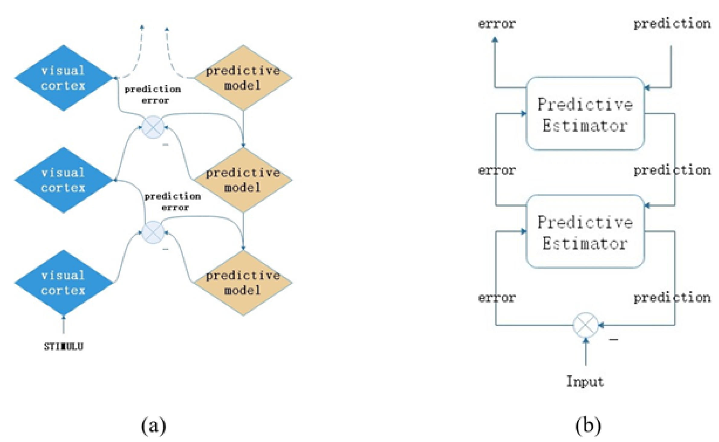It has been applied in building computational models to explain different perceptual and neurobiological phenomena of the visual cortex [11]. Specifically, it describes a simple hierarchical computational framework: neurons at a higher level propagate predictions downwards, whereas neurons at a lower level propagate prediction errors upwards [12], as shown in Figure 2. The entire model is updated through a combination of bottom-up and top-down information flows, so it does not rely solely on external information. Furthermore, the propagation of prediction errors constitutes effective feedback, allowing the model to perform self-supervised learning. The above characteristics make the predictive coding framework available and valuable to apply to the field of signal processing. For example, Whittington et al. proposed that a network developed in the predictive coding framework can efficiently perform supervised learning with simple local Hebbian plasticity. The activity of the prediction error node is similar to the error term in the backpropagation algorithm, so the weight change required by the backpropagation algorithm can be approximated by means of a simple Hebbian plasticity of connections in the prediction encoding network [13].

In the field of visual-frame prediction, substantial work has been conducted on the basis of predictive coding. One of most successful applications is the PredNet model, proposed by Lotter et al. [15]. It is a ConvLSTM-based model which stacks several ConvLSTMs vertically to generate the top-down propagation of predictions. On the other hand, a bottom-up propagation process delivers the error values.This model achieved state-of-the-art performance in a few tasks, such as video-frame prediction. Elsayed et al. [16] implemented a novel ConvLSTM-based network called the Reduced-Gate ConvLSTM, which showed better performance. However, although these works strictly followed the predictive coding style, the details were not adequately taken into account. The predictive coding computational framework only roughly explains how the brain works, but some details, such as transmission delays, are ignored. The transmission delay has been discussed in the work of Hogendoorn et al. [17] in detail. They pointed out that only when the concept of transmission delay is added can a predictive coding model be regarded as a temporal prediction model. In addition, other neuroscientific phenomena, such as the different frequencies of oscillations in different levels of the cortex, are equally important. Therefore, we designed a video prediction method with a comprehensive consideration of the different biological evidence mentioned above.

In addition to the above methods, more predictive models have been proposed, building on the recent success of deep learning. The early state-of-the-art machine learning techniques are usually based on encoder-decoder training. Using an end-to-end training method, consecutive frames are used as inputs and outputs to train visual offsets or their coherent semantic meanings. On the basis of the encoder-decoder network and LSTM, Villegas et al. proposed a novel method which decomposes the motion and content [18], and which encodes the local dynamics and the spatial layout separately, so as to simplify the task of prediction. However, the motion referred to is simply obtained by subtracting $x_{t-1}$ from $x_t$. It describes changes at the pixel level only. Jin et al. [19] also explored inter-frame variations, in an approach which is similar to that of MCNet. Their innovation was the use of GDL (gradient difference loss) regularization as a loss function to sharpen their predictions. In addition, Shi et al. also implemented the use of an CNN-LSTM-based model for precipitation nowcasting [20]. Unlike the previous two works, they embedded convolutional neural networks directly into the LSTM, which led to better performance in capturing spatial-temporal correlations, and this approach has also been adopted into our network architecture.

Moreover, training in an adversarial fashion is another popular method, since the use of GAN (generative adversarial network) shows excellent performance in image generation for predictions. For example, Aigner et al. [21] proposed the FutureGAN method based on the concept of PGGAN (progressive growing of GANs) in 2018. They extended this concept to the task of visual-frame prediction using a 3D convolutional encoder-decoder model to capture the spatial-temporal information. However, 3D convolution undoubtedly consumes more computational resources than other methods. Before PredNet, Lotter et al. also proposed a GAN-based model named a predictive generative network (PGN), which was trained in [22] with a weighted MSE and adversarial loss approach for visual-frame prediction.

In summary, there are two main problems with the previous studies in this area of research. (1) There is still room for improvement in terms of network structure and training strategies. For instance, the encoder-RNN-decoder network only performs predictions in the high-level semantic space, meaning that most of the low-level details are ignored. (2) The computational cost is too high, with these methods consuming a lot of resources (especially during training). The question of how to reduce the computational overhead through reasonable pruning is also important. We have previously introduced the characteristics of predictive coding and the related theories, which provide an efficient and reliable theoretical computing framework. Therefore, in order to reduce the consumption of resources and achieve sustainable artificial intelligence, we suggest combining this efficient cognitive framework and advanced data-driven machine learning methods to design an efficient predictive network model, which can not only improve predictive accuracy, but also reduce computational costs. Next, we will introduce our model in detail.

3. Network Model and Methods

In this section, we introduce the cognition-inspired model, which is specialized for visual-frame frame predictions. As its name (PPNet) suggests, its pyramid-like architecture is beneficial to predicting visual frames, as the neurons on the lower levels encode and predict the actual frames and the neurons on top encode the scenarios, which usually only change within a few visual frames (Figure 3). We explain this idea in the next subsection. Then, the detailed architecture, as well as the algorithm, are introduced in the subsequent subsections.

3.1. Efficiency in the Pyramid Architecture

In this work, we mainly referred to the design concept of PredNet [15] when building the network structure. As early as 2016, Lotter et al. proposed such a typical predictive coding model, which strictly follows the dual-way flow at every time-step and which has achieved outstanding performance. Nevertheless, the processing of information can be improved in at least two aspects.

First, according to predictive processing framework, at least two kinds of neurons are required: an internal representation neuron for generating predictions and an error calculation neuron for computing prediction errors. In the PredNet model, bottom-up inputs at each level only served as targets of error calculation neurons for the performance of comparisons with top-down predictions to generate prediction errors, and the information that was propagated upward was related only to the prediction error itself. However, we argue that it is necessary to use the past and present sensory information (represented here as video frames) as the inputs of the representation neurons to generate predictions with higher accuracy. The formed memory can be formulated in a Bayesian framework, which is necessary to use in order to generate predictions. Through the use of such a Bayesian model in the learning process, we can maximize the marginal likelihood or the entropy [23].

Second, as a cognitively inspired model, we suggest that such predictions and sensory inputs can be respectively implemented in at least two information streams in a hierarchical manner. This not only is inspired by the human nervous system, but it is also a way to integrate inputs from different network layers to obtain more spatiotemporal information—an approach which has also been widely used in deep learning architectures such as ResNet, DenseNet and so on.

Based on the above assumptions, we have proposed and designed a predictive model in which the updating ratesof neurons on different levels can differ. Alternatively, this can be also interpreted as a delay in information transmission. In general, it takes time for information to be transmitted from a lower level to a higher level, so there is a delay in transmissions between different layers. However, neurons at the bottom layer do not passively wait for information transmitted from the top layer before making a prediction. The changes in biological synapses are determined only by the activity of presynaptic and postsynaptic neurons [13]. Therefore, in PPNet, once the prediction unit (ConvLSTM) receives a sensory input (green), it will immediately combine this with the prediction from a higher level (if any) to make predictions. As we mentioned in Section 2, the delay in information transmission has been discussed in detail in the work of Hogendoorn et al. [17]. They argue that traditional predictive coding models such as the one first proposed by Rao and Ballard [14] do not predict the future, but hierarchically predict what is happening. When the concept of a transmission delay is added, the task of the predictive coding model changes from hierarchical prediction to temporal prediction.

As a result, PPNet could be regarded as an equivalent to the large-scale brain network (LSBN) in which the higher cognitive function is conducted in a higher level of the deep learning network. According to the neuroscientific evidence, such a cognitive function which is processed in the PFC (prefrontal cortex) can be also used to predict the situated scenarios in our visual-frame prediction application for an agent.Therefore, our model is built considering the balance between biological evidence and efficiency in computing.

3.2. Network Architecture

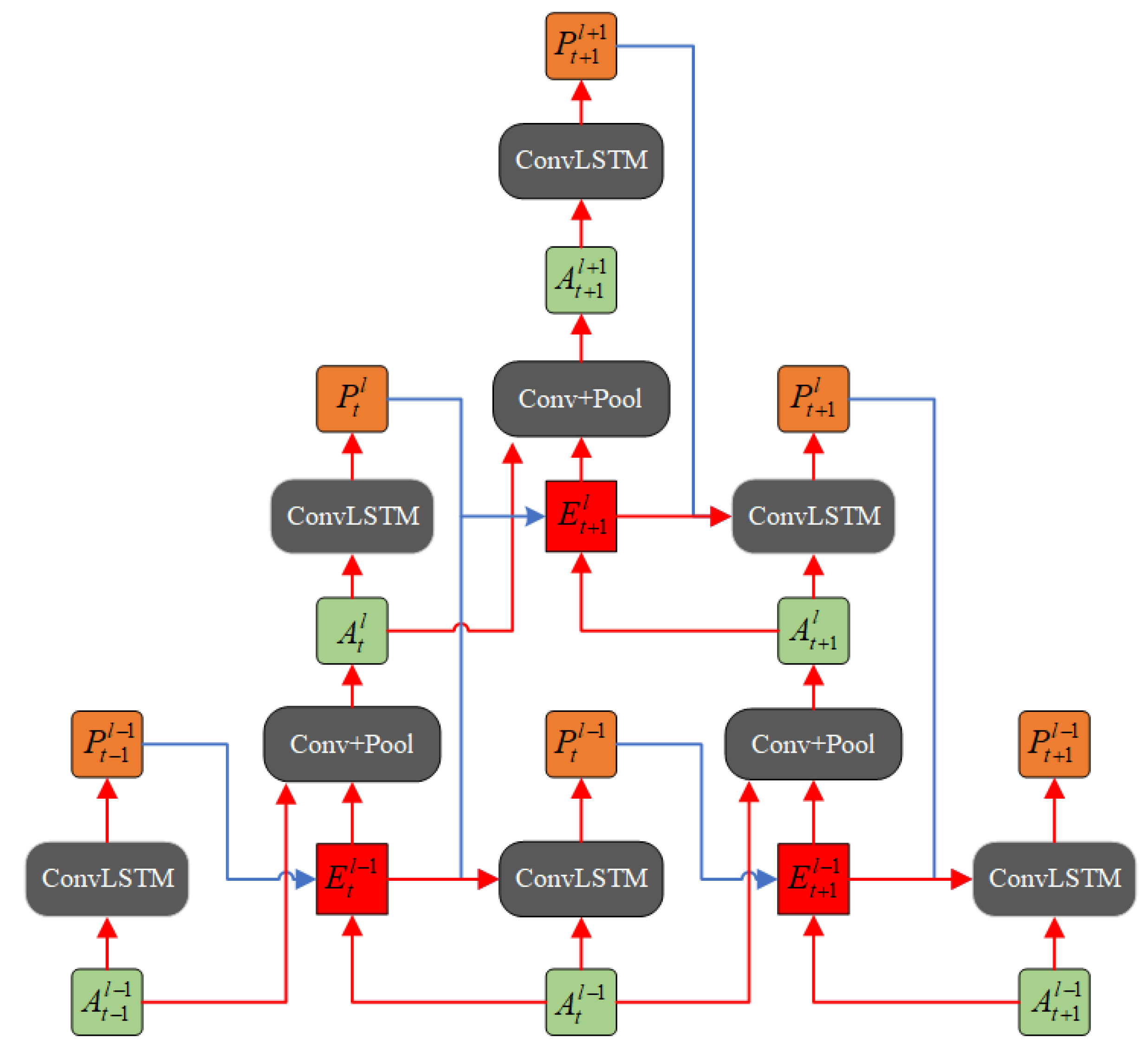
In this section, we introduce our network model in detail. The architecture of our model is shown in Figure 3. For the sake of understandability, it is necessary to state the meanings of the symbols in the figure before conducting a detailed comparison and analysis.

• ${\mathit{A}}_{\mathit{t}}^{\mathit{l}}$: depicted in green, represents the sensory input at level $\mathit{l}$ and time step $\mathit{t}$;
• ${\mathit{P}}_{\mathit{t}}^{\mathit{l}}$: depicted in orange, represents the prediction at level $\mathit{l}$ and time step $\mathit{t}$. Its prediction object is the sensory input at level $\mathit{l}$ and time step $\mathit{t}$ (${\mathit{A}}_{\mathit{t}+\mathit{1}}^{\mathit{l}}$); and
• ${\mathit{E}}_{\mathit{t}}^{\mathit{l}}$: depicted in red, represents the prediction error at level $\mathit{l}$ and time step $\mathit{t}$. It is calculated based on the previous prediction ${\mathit{P}}_{\mathit{t}-\mathit{1}}^{\mathit{l}}$ and the current sensory input ${\mathit{A}}_{\mathit{t}}^{\mathit{l}}$.

Inspired by PredNet, PPNet also uses ConvLSTM componentsas its basic components, as they provide prediction flows with long-term dependency. Similarly, each layer of the network can be roughly divided into three parts:

• A predictive unit, which is made up of the recurrent convolutional network (ConvLSTM). It receives a sensory input ${\mathit{A}}_{\mathit{t}}^{\mathit{l}}$ and a prediction ${\mathit{P}}_{\mathit{t}}^{\mathit{l}+\mathit{1}}$ from higher level (if any), to generate a local prediction ${\mathit{P}}_{\mathit{t}}^{\mathit{l}}$ of next time step.
• A generative unit, which consists of a convolutional layer and a pooling layer. This unit is responsible for turning the local input ${\mathit{A}}_{\mathit{t}}^{\mathit{l}}$, as well as the prediction error ${\mathit{E}}_{\mathit{t}+\mathit{1}}^{\mathit{l}}$, into the input ${\mathit{A}}_{\mathit{t}+\mathit{1}}^{\mathit{l}+\mathit{1}}$ of the next level.
• An error representation layer, which is split into separate rectified positive (${\mathit{A}}_{\mathit{t}}^{\mathit{l}}-{\mathit{P}}_{\mathit{t}}^{\mathit{l}}$) and negative (${\mathit{P}}_{\mathit{t}}^{\mathit{l}}-{\mathit{A}}_{\mathit{t}}^{\mathit{l}}$) error populations.

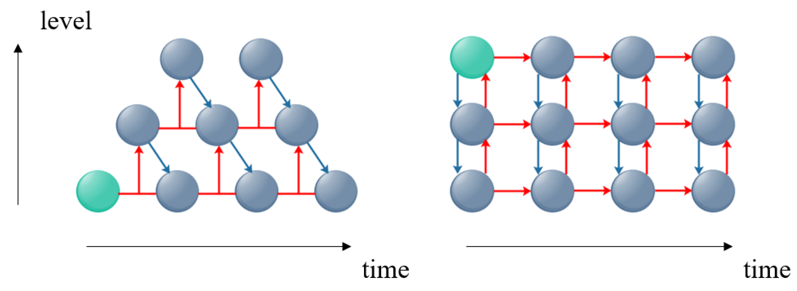
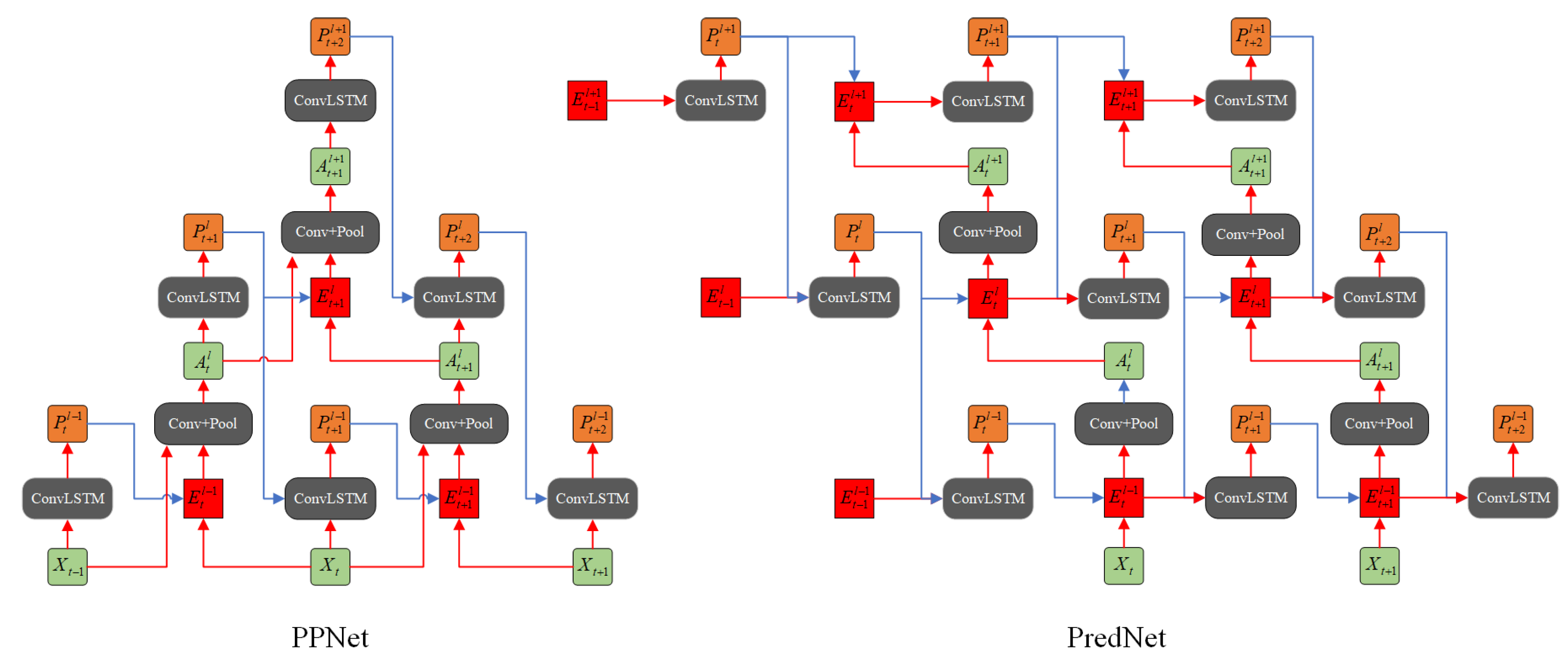
In order to process the prediction only when it is necessary, we show that the dual-direction propagationcan be carried out in a more efficient way. For a better understanding and comparison, a diagram (Figure 4) is provided below regarding the ways in which information propagates, comparing our model and the PredNet model.

First, the computation process of our model begins at the lowest layer after receiving the first sensory input. This is consistent with the design concept mentioned in Section 3.1, which is different from that of PredNet, which first starts at the top level by generating a prediction without any prior information. Second, in our model, the bottom-up input of a higher-level unit comes from the combination of information from the lower-level units of two time-steps. Specifically, the current input ${\mathit{A}}_{\mathit{t}}^{\mathit{l}}$ is fed into internal representation neuron (ConvLSTM) to generate a local prediction ${\mathit{P}}_{\mathit{t}}^{\mathit{l}}$ at the time step $\mathit{t}$, which is then compared with the next time step input ${\mathit{A}}_{\mathit{t}+\mathit{1}}^{\mathit{l}}$ to generate the prediction error ${\mathit{E}}_{\mathit{t}+\mathit{1}}^{\mathit{l}}$. In other words, ${\mathit{A}}_{\mathit{t}+\mathit{1}}^{\mathit{l}}$ is not only a bottom-up sensory input for an internal representation neuron at time step $\mathit{t}+\mathit{1}$, it is also the target of the previous step $\mathit{t}$, which is different from PredNet (in which ${\mathit{A}}_{\mathit{t}+\mathit{1}}^{\mathit{l}}$ serves merely as a target at time-step $\mathit{t}+\mathit{1}$).

Note that with both the prediction (${\mathit{P}}_{\mathit{t}}^{\mathit{l}}$) and the target (${\mathit{A}}_{\mathit{t}+\mathit{1}}^{\mathit{l}}$) PPNet can generate a prediction error for upward propagation. That is, at least two continuous sensory inputs ${\mathit{A}}_{\mathit{t}}^{\mathit{l}}$ and ${\mathit{A}}_{\mathit{t}+\mathit{1}}^{\mathit{l}}$ are required to generate a prediction error for upward propagation, with the former serving as an input to produce the prediction, whereas the latter serves as a target. As a result, the computations of neurons at different levels are not updated in a synchronized way at different levels, and the update frequency of neurons decreases as the network level increases, which is consistent with the biological evidence: deep neurons oscillate at a lower frequency [24]. For this reason, the bottom-up input of the top level contains information for multiple time-steps at the bottom-level, which means that PPNet has a stronger temporal correlation in its structure, rather than relying solely on the temporal correlation of LSTM. In addition, it allows PPNet to reduce the computational load by not having to update higher-level neurons.

3.3. Training Loss and Adaptive Weight

The training loss in our model is defined as the concatenation of positive and negative errors (Equation (1)), where $\widehat{Y}$ denotes a prediction and Y is a target. $ReLU$ denotes the “rectified linear activation function”, which is defined in Equation (2). $concat$ refers to concatenating two multidimensional matrices together (for example, concatenating two matrices of dimension (b, c, h, w) into a matrix of (b, 2c, h, w)). 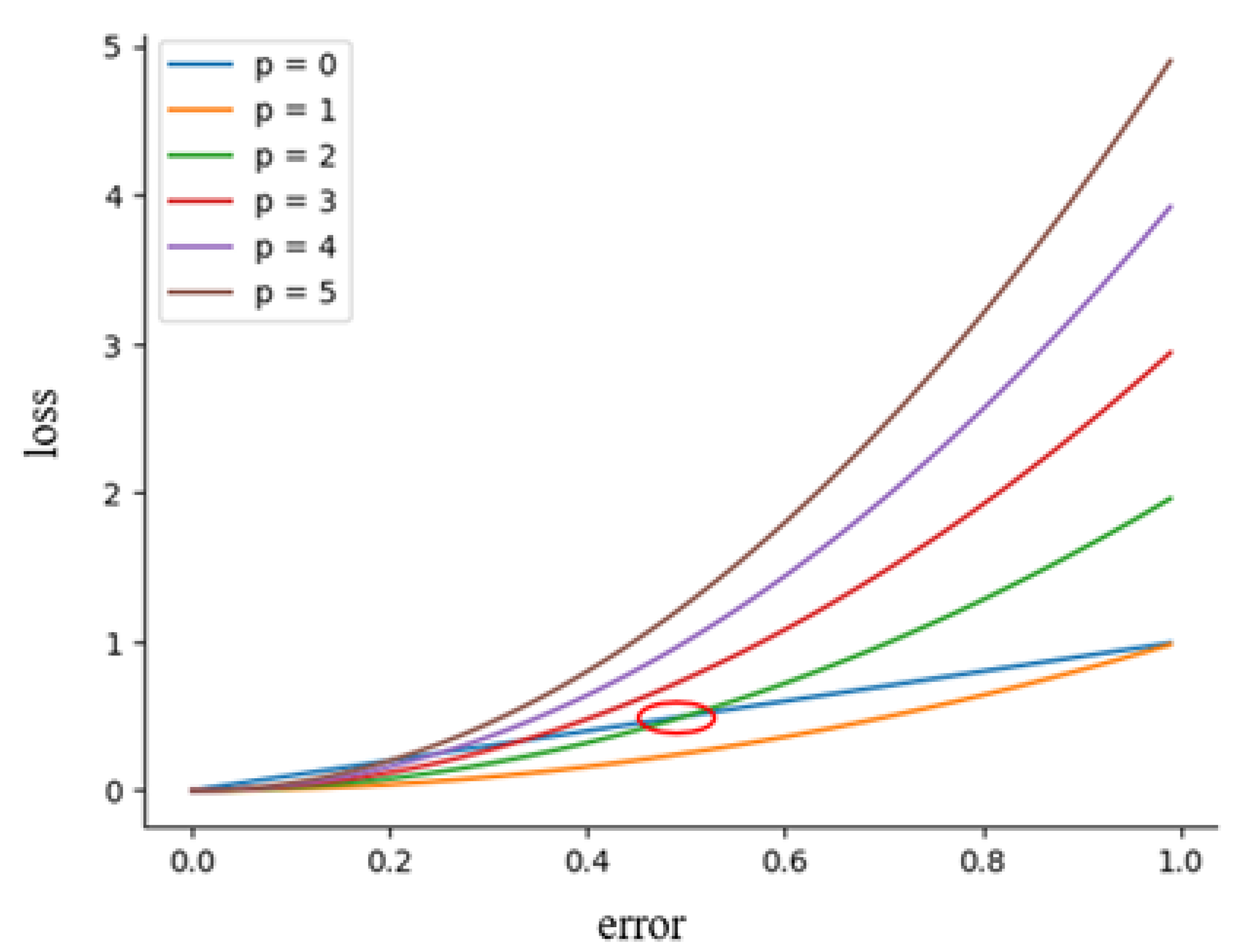Equation (1) indicates the error population in the neurons, incorporating both positive errors and negative errors [14]. Furthermore, to sharpen the predictions, we introduce an adaptive weight into the loss function, inspired by the attention mechanism.

$$E_t=concat[ReLU(\widehat{Y}-Y),ReLU(Y-\widehat{Y})]$$

(1)

$$f\left(x\right)=\left\{\begin{array}{cc}0,\hfill & x\le 0\hfill \\ x,\hfill & x>0\hfill \end{array}\right.$$

(2)

At the beginning of the visual sequences, the error is usually quite large since it drives the top-down prediction to minimize the error. That is, the greater the prediction error, the stronger the brain response. We argue that the brain’s response can be seen as a weighting of the prediction error. Based on this idea, we propose to add more weights to increase the contributions of prediction errors with higher values (for example, at the beginnings of sequences). When one has a lower value, itscontribution is reduced. A set of experiments performed by Kutas & Hillyard [25] showed that, when a prediction was seriously inconsistent with the environment, the brain reacted more strongly. Higher accuracy means less uncertainty, which is reflected in a higher gain in the relevant error units to complete the update.In other words, the error units become more adaptive, driving learning and plasticity, if they are given an increasing weight. Therefore, we have introduced a method of adaptive weights into our model, with a higher value of the prediction error resulting in a higher weight.

$$W_t=p{E}_t$$

(3)

$${\mathcal{L}}_{AW}=\sum _1^{T-1}{\lambda }_t{W}_t{E}_t$$

(4)

The adaptive weight for every time-step is calculated by directly multiplying the error itself by a coefficient (shown in Equation (3)). $E_t$ denotes the prediction error at time step t, whereas p is a changeable hyper-parameter. Thus, the training loss is defined as in Equation (4), where T denotes the length of input sequences and ${\lambda }_t$ denotes the weighting factors by time. However, the error with a value less than $1/p$ will become smaller after being weighted. 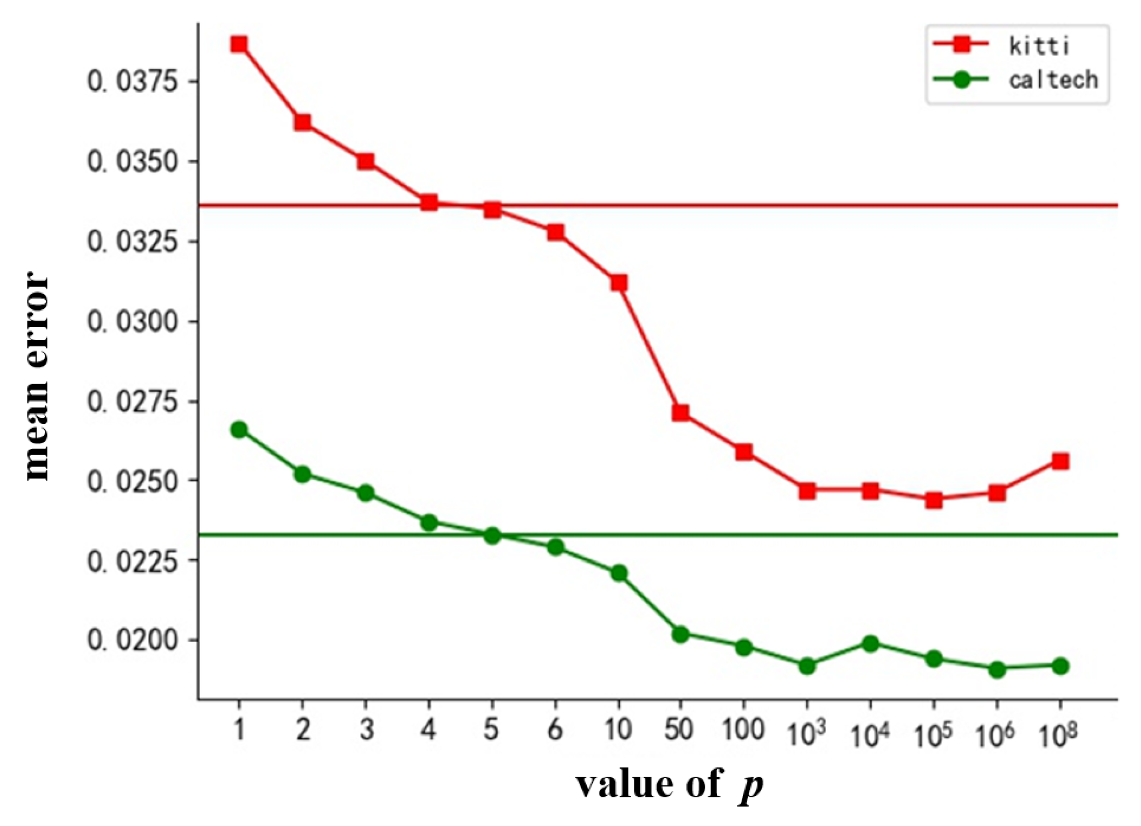Figure 5 shows the relationship between p and the loss. When the error is greater than the threshold (e.g., the intersection of the red circle), it will be enlarged. However, it will be reduced if it is less than the threshold. From an attention mechanism perspective, we pay more attention to errors that are larger than the threshold and pay less attention to errors that are smaller than the threshold. Therefore, the choice of threshold is extremely important. We further explore the influence of the hyper-parameter p in the following experiments.

3.4. Algorithm

In this section, we introduce the algorithm to implement the above model based on the architecture and computation process mentioned in Section 3.2. To better serve the following description, we reiterate the definition of each parameter as follows.

• ${\mathit{E}}_{\mathit{t}}^{\mathit{l}}$: The prediction error;
• ${\mathit{H}}_{\mathit{t}}^{\mathit{l}}$: The combination of hidden state ${\mathit{h}}_{\mathit{t}}^{\mathit{l}}$ and cell state ${\mathit{c}}_{\mathit{t}}^{\mathit{l}}$;
• ${\mathit{A}}_{\mathit{t}}^{\mathit{l}}$: The input, as well as the target, of each layer;
• ${\mathit{x}}_{\mathit{t}}$: The image at frame $\mathit{t}$ in the input sequence;
• ${\mathit{P}}_{\mathit{t}}^{\mathit{l}}$: The prediction; and
• $\mathit{T}$: The length of the input sequence.

$$A_t^l=\left\{\begin{array}{cc}{x}_t,\hfill & \mathrm{if}l=0\hfill \\ MaxPool\left(ReLU\left(Conv(E_t^{l-1},A_{t-1}^{l-1})\right)\right),\hfill & \mathrm{if}l>0\hfill \end{array}\right.$$

(5)

$$H_{t+1}^l=ConvLSTM(A_t^l,H_t^l,upsample\left(P_{t+1}^{l+1}\right))$$

(6)

$$h_{t+1}^l,c_{t+1}^l=H_{t+1}^l$$

(7)

$$P_{t+1}^l=ReLU\left(Conv\left(h_{t+1}^l\right)\right)$$

(8)

$$E_{t+1}^l=[ReLU(P_{t+1}^l-A_{t+1}^l);ReLU(A_{t+1}^l-P_{t+1}^l)]$$

(9)

The complete algorithms are listed in Equations (5) to (9). The model is trained to minimized the training loss, defined as in Equation (5), and our implementation is described in Algorithm 1. The information flows through two streams: (1) a top-down propagation, in which the hidden states $H_t^l$ of ConvLSTM are updated and the local prediction $P_t^l$ is generated, and (2) a bottom-up stream in which the prediction error $E_{t+1}^l$ is calculated and propagated up to a higher level, along with the local input $A_t^l$. Due to the pyramid design, the computation in our network updates the lowest layer (i.e., layer 0) at the first time-step. However, for the convenience of programming, we refer to the programming method of PredNet and thus perform the calculation of the top-down information flow first (lines 2–11 in Algorithm 1), and then calculate the prediction error and update the sensory input of the higher level (lines 12–19 in Algorithm 1). In contrast, if there is no sensory input $A_t^l$ at time-step t and level l, the calculation of this predictive unit is skipped without generating any predictions and the hidden state of ConvLSTM $H_t^l$ stays the same.

Algorithm 1: Calculation of the Pyramidal Predictive Network

4. Experiments

In this section, several experiments are presented to illustrate the performance of the PPNet, using datasets related to autonomous driving. We first introduce the features and pre-processing methods of the three datasets—KTH, Caltech Pedestrian and KITTI—which are commonly used in visual-frame prediction tasks. Then the training details and evaluations comparing PPNet and other state-of-the-art models are presented in the subsequent subsections.

4.1. Datasets and Pre-Processing

All the aforementioned datasets had to be processed into sequences before they could be used for training. In this section, we introduce the features of these datasets, as well as the pre-processing methods used.

• KTH: The KTH dataset is a relatively old dataset, made in 2004 for the recognition of human actions. However, it is still very popular in the research of visual-frame prediction because of its simple scenarios end events.
• KITTI: The KITTI dataset is one of the most widely-used datasets for autonomous driving. It includes various processed data, but we directly downloaded its raw images for training. Approx. 35 K frames were used for training and 4.5 K were used for testing. The frames were center-cropped and resized to $128\times 160$ pixels in the same way as PredNet. Compared to the other two datasets, the interframe variations in this dataset were greater.
• Caltech Pedestrian: This dataset was originally designed for pedestrian detection, and is also suitable for the work of visual-frame prediction. The frames were directly resized to $128\times 160$ pixels, which is the same as the KITTI images. The interframe variations of this dataset are much smaller than those of KITTI, which might result in the model learning a repetition instead of prediction.

4.2. Training Setting

We implemented the PPNet using the PyTorch platform and trained it on a Geforce RTX 3070 GPU. The length of the input sequence was set to 10 and the number of layers in the network was set to sex. Other hyper-parameters are shown in

Table 1. Hyper-parameters for training, including the training epoch, learning rate and hyper-parameters p and ${\lambda }_t$, defined in Section 3.3.

Hyper-Parameters	Datasets
	KITTI	Caltech Pedestrian	KTH
epoch	300	200	200
learning rate	0.0002
P	${10}^4$	${10}^4$	${10}^3$
${\lambda }_t$	${\lambda }_t=\left\{\begin{array}{cc}0.5,\hfill & \mathrm{if}t=0\hfill \\ 1,\hfill & \mathrm{if}t>0\hfill \end{array}\right.$

. Influenced by initialization, the time-weight ${\lambda }_t$ of the prediction error generated at the first time step was set to 0.5, whereas the rest were set to 1.

In order to select a suitable value for the hyper-parameter p, as proposed previously, we performed two sets of experiments using part of the KITTI dataset and the Caltech Pedestrian dataset to explore its influence. The results are shown in Figure 6. The horizontal lines indicate the results obtained without adding any weight. According to Equations (2) and (4), when the value of p was set to 1, the loss function was equivalent to the mean square error loss. Obviously, the method of dividing the error into positive error and negative error was indeed beneficial. Better results could be observed when the value ofp was greater than five (or six) compared to those obtained without any weighting. The training loss (mean error) decreased with the increase inp, and we obtained a result close to the best result when its value was close to ${10}^3$ However, continuing to increase its value may have resulted in the opposite performance. Therefore, we chose a value around ${10}^3$ for the subsequent experiments.

4.3. Evaluation Results

In this section, we used SSIM [26], PSNR [27] and LPIPS [28] for quantitative evaluations. SSIM is an early measure of image similarity, which compares two images from the perspective of brightness, contrast and structure. PSNR is also a metric for evaluating image quality. It measures the degree of image distortion by calculating the ratio of the maximum signal to background noise. However, the above two evaluation indicators have the same problem: the results may not match the evaluations performed by the human visual system [29]. To solve this problem, Zhang et al. proposed the LPIPS metric to try to simulate the evaluations performed by the human visual system. Higher values indicate better results for SSIM and PSNR, whereas lower values indicate better results for LPIPS.

Results for the KTH dataset:

Table 2. The quantitative evaluation results obtained on the KTH dataset. The results were averaged for 10 future time steps ($10\to 20$) and 30 time steps ($10\to 40$), respectively.

Methods	0 → 5			0 → 15
	SSIM ↑	PSNR ↑	LPIPS ↓	SSIM ↑	PSNR ↑	LPIPS ↓
MCNet [18]	0.804	25.95	-	0.73	23.89	-
fRNN [32]	0.771	26.12	-	0.678	23.77	-
PredRNN [33]	0.839	27.55	-	0.703	24.16	-
PredRNN++ [34]	0.865	28.47	22.89	0.741	25.21	27.90
VarNet [19]	0.843	28.48	-	0.739	25.37	-
E3D-LSTM [35]	0.879	29.31	29.84	0.810	27.24	32.88
Conv-TT-LSTM [30]	0.907	28.36	13.34	0.882	26.11	19.12
LMC-Memory [31]	0.894	28.61	13.33	0.879	27.50	15.98
Ours	0.886	31.02	13.12	0.821	28.37	23.19

shows the quantitative evaluation results obtained with the state-of-the-art methods on the KTH dataset. Similarly to previous works, we made calculations based on the average results obteined over 10 future frames ($10\to 20$) and 30 frames ($10\to 30$), respectively, with 10 input frames. Our method achieved better or comparable results compared with the state-of-the-art works in terms of accuracy assessments. However, in the video prediction tasks, its pure quantitative evaluations seemed to be weak sometimes. Therefore, we also visualized the predicted results. Figure 7 shows examples of the predictions of our method and those of other proposed methods. Obviously, our method also achieved good results from the perspective of the human visual system evaluation, whereas Conv-TT-LSTM [30], which has acquired outstanding performance in quantitative evaluations, performed poorly from the perspective of visual presentation (in fact, it also performed poorly in another work [31]). This is a common problem in video prediction tasks. In such tasks there is not an accurate and uncontroversial evaluation metric, as in the case of image classification or semantic segmentation. As a result, it was necessary to combine the quantitative evaluation and the qualitative evaluation to make a better comparison.

Results for the Caltech and KITTI datasets: We also validated our methods on the Caltech and KITTI datasets, which contain more complex scenarios and events.

Table 3. The quantitative evaluation results obtained for the Caltech and KITTI datasets, respectively. The results were averaged for 5 future time steps ($10\to 15$).

Methods	Caltech 10 → 15			KITTI 10 → 15
	SSIM ↑	PSNR ↑	LPIPS ↓	SSIM ↑	PSNR ↑	LPIPS ↓
MCNet [18]	0.705	-	37.34	0.555	-	37.39
PredNet [15]	0.752	-	36.03	0.475	-	62.95
Voxel Flow [36]	0.711	-	28.79	0.426	-	41.59
Vid2vid [37]	0.751	-	20.14	-	-	-
FVSOMP [38]	0.756	-	16.50	0.608	-	30.49
Ours	0.812	21.3	14.83	0.617	18.24	31.07

shows the quantitative evaluation results. Obviously, even though we only counted the predicted frames of five future time-steps, the results were still much worse than the performance on KTH. In fact, this is related with how complex and varied the scene is. The more complex the scene and the greater the variation, the more difficult it is to predict. As shown in Figure 8, we visualized the inter-frame variations of the three datasets separately. The Caltech dataset has a similar level of sophistication as KITTI, but KITTI is more variable than Caltech and therefore the methods performed worse on KITTI. Achieving predictions in complex scenes is also an urgent problem to be solved in relation to current video prediction tasks.

Comparison with PredNet As we mentioned above, PredNet strictly follows the computational style of a traditional predictive coding framework, and the network structures of PPNet and PredNet are similar (for example, both use ConvLSTM as their backbone). The PredNet model is redrawn in the same way as our model in Appendix A. Therefore, it is relatively easy to set the same parameters, such as network depth and width, to retrain PredNet and make a fair and clear comparison, which can be considered an ablation study, to highlight the rationality and superiority of our model.

Table 4. Evaluation of next-frame predictions for each dataset. We undertook comparisons in terms of prediction accuracy and the computational overhead.

Metrics	KTH		Caltech		KITTI
	Ours	PredNet	Ours	PredNet	Ours	PredNet
SSIM ↑	0.945	0.934	0.919	0.887	0.787	0.642
PSNR ↑	36.47	33.31	28.44	23.56	21.96	16.58
LPIPS ↓	8.03	8.92	7.35	14.65	21.49	38.51
Time/ms ↓	27.6	52.2	37.0	71.4	37.2	71.5

shows the models’ next-frame prediction performance on the KTH, Caltech and KITTI datasets, respectively. Obviously, our method’s performance was superior to that of PredNet in terms of both its prediction accuracy and computational overhead. The pyramid style is effective. By reducing the oscillation frequency, not only can higher-level neurons obtain longer-term information, but this approach can also reduce the computational cost.

Figure 9 visualizes the long-term predictions for each dataset with different predicted time steps, respectively. In general, our results were better than those of PredNet. First, it can be seen in the figure that the inter-frame variations of the KITTI dataset were much larger than those of the other two datasets, and both PPNet and PredNet made fuzzy predictions for this dataset. However, PPNet could still make better predictions in the first few steps, whereas PredNet made blurry predictions and then merely reproduced them. This kind of replication is more obvious when using the Caltech dataset for evaluation. Though generating clearer frames compared to our method, PredNet merely reproduced previous frames, instead of making predictions. On the contrary, PPNet was still able to capture the motion information in the input sequences and make authentic predictions. PredNet captured the motion information on the KTH dataset eventually, but it learned only the person’s direction and their approximated speed, whereas other subtle movements, such as the actions of the person’s arm and leg, were lost.

In summary, we have presented several experiment results to show the remarkable performance of our method, which was superior to that of PredNet in terms of its prediction accuracy, computational cost and visual presentation. In addition, we were also able to obtain results equal to or better than the other state-of-the-art methods, thus indicating the superiority of our method.

5. Discussion

5.1. Propagation of Weighted Errors

Additional experiments were performed to explore the influence of the propagation of prediction errors. As mentioned above, the prediction errors propagate upward to a higher level. This leads to the question of which errors should be passedupward—the original errors or the weighted errors? It is necessary to indicate that the results shown in Figure 6 were those in which the original errors were transmitted upward and the weighted errors were only propagated backward. We obtained a worse result when we propagated the weighted errors both upward and backward after being normalized (

Table 5. The mean errors (ME) obtained using different methods of propagation.

Value of p		5	10	100	1000	10,000
backward	kitti	0.0335	0.0312	0.0259	0.0247	0.0247
	caltech	0.0233	0.0221	0.0198	0.0192	0.0199
backward and upward	kitti	0.0450	/	/	0.0463	0.0460
	caltech	/	0.0303	0.0311	0.0316	/

). As Corlett [39] and Fletcher et al. [40] have speculated, errors may be “false” after being weighted. Profound corrections would be made to our model of the world if waves of persistent and highly weighted “false errors” were propagated upward. Using the adaptive weights proposed in Section 3.3, we have provide a possible proof for this assumption from the perspective of an artificial neural network.

5.2. The Efficiency of the Pyramid-like Architecture

A set of priors is often already active on a higher level of the cognitive hierarchy, poised to impact the processing of new sensory inputs without further delay when contextual information has been put in place.Similarly, there is a delay in the upward flow of information at the beginning, but this disappears once the information reaches the highest level in our model, which may result in a trivial reduction of the computational cost when the input sequence is long enough. However, long sequences are not required. LSTM networks may capture spurious long-term dependencies that may have been present in the training data, hence learning inadequate causal models [41]. Additionally, we performed a set of experiments on both PPNet and PredNet, processing the same data into sequences with different lengths to prove our point (note that the total number of video frames was constant). As shown in Figure 10, the length of the input sequence had little effect on the prediction accuracy, but less time was required when using a shorter sequence in our proposed PPNet. Therefore, we can process the data into shorter sequences during training to reduce the consumption of resources and achieve sustainable artificial intelligence.

6. Conclusions

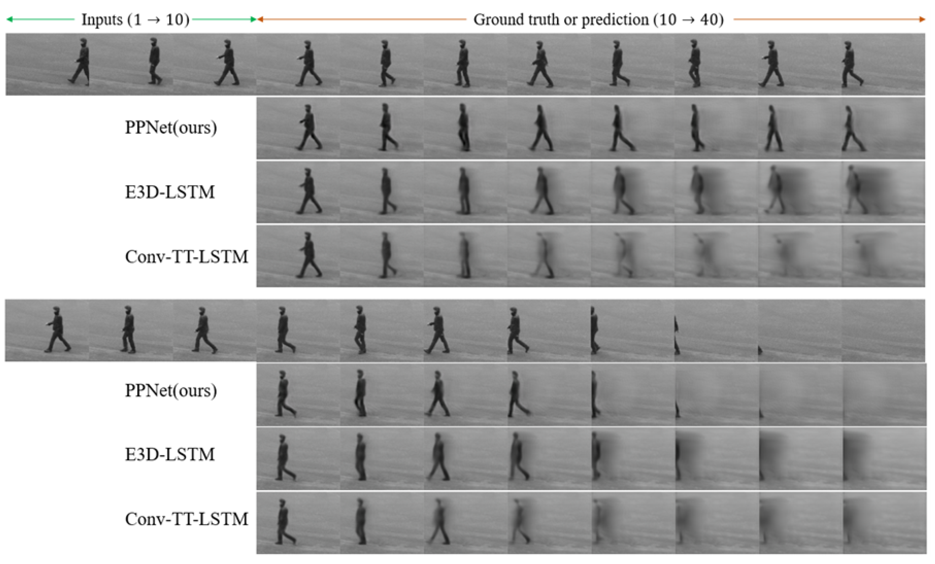
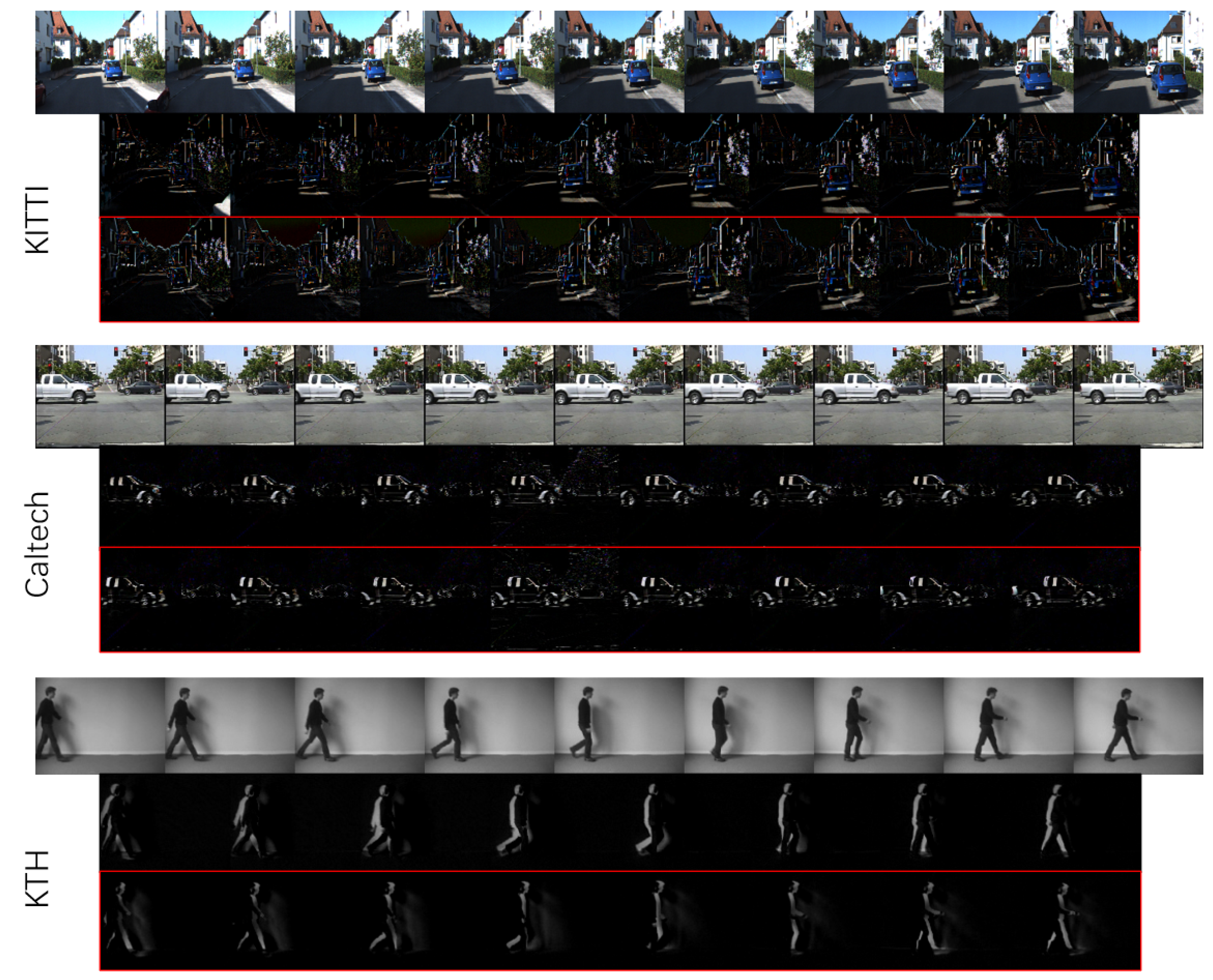
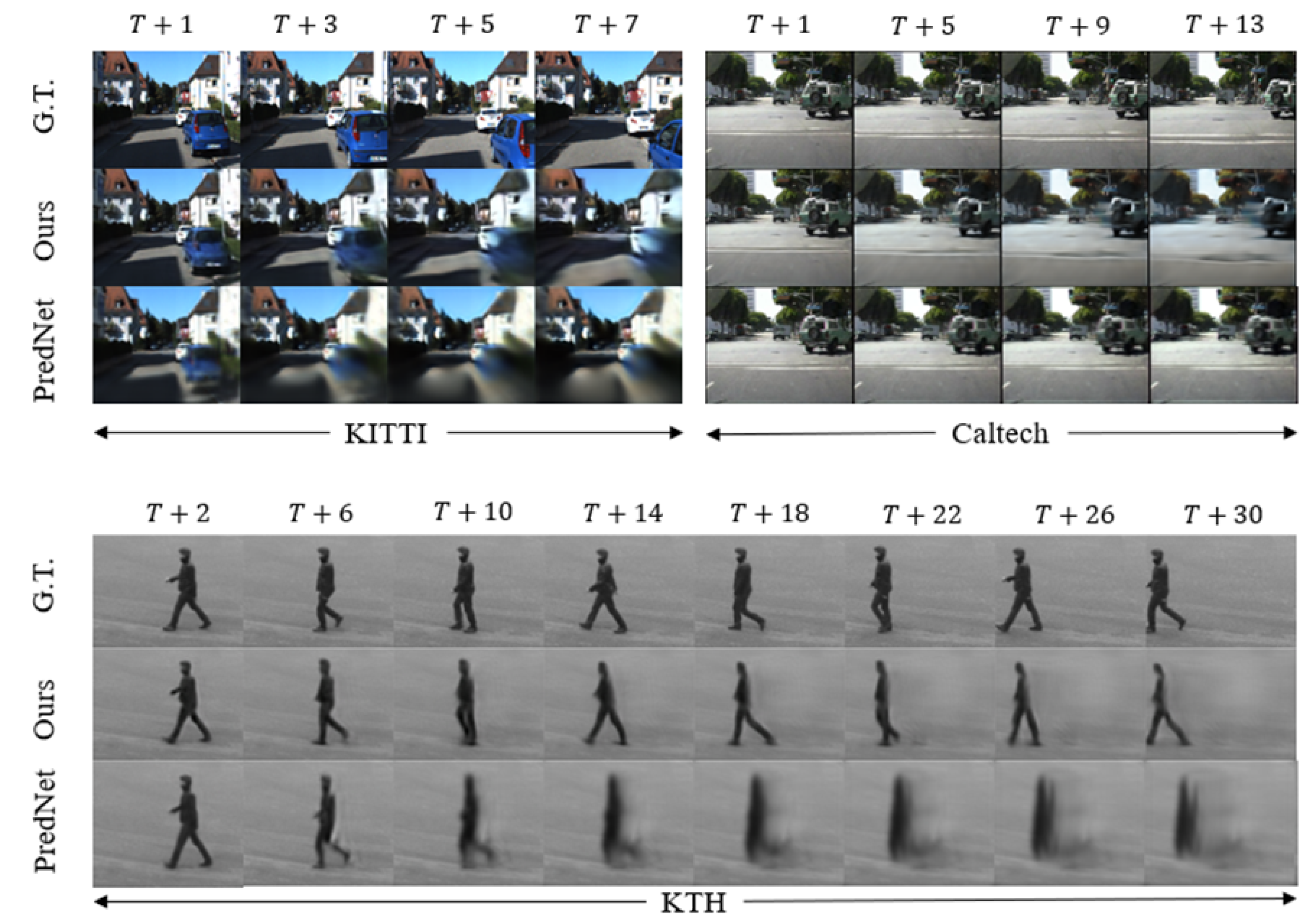
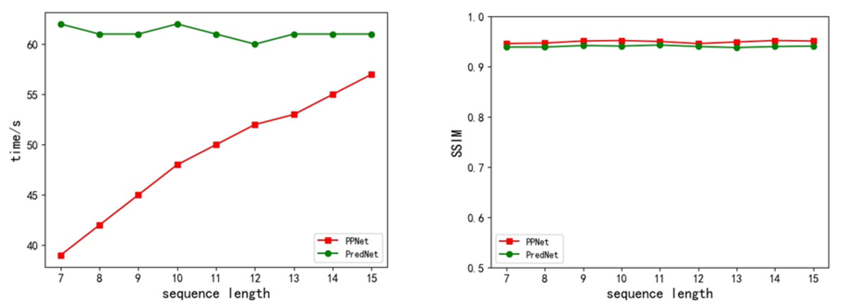
In this paper, we have demonstrated the use of a pyramidal predictive network for visual-frame prediction based on the predictive coding concept, along with the consideration of efficient computational performance. This model encodes information at various temporal and spatial scales, with an up-down propagation of predictions and a bottom-up propagation of the combination of sensory inputs and prediction errors. It has a stronger temporal correlation in its structure and requires lower computation costs. We analyzed the rationality of the model in detail from the perspectives of predictive processing and machine learning. Importantly, this proposed model achieved a remarkable performance compared to state-of-the-art models, according to the experimental results.

Nevertheless, there is still room for improvement of the proposed model. In the long-term forecasting process, false “prediction errors” may cause the model to average the possible future predictions into a single, fuzzy forecast, which is an urgent problem existing in most predictive models. In addition, performing predictions on the basis of directly predicting natural visual frames is still a challenging task due to the curse of dimensionality. Therefore, in the future, we intend to reduce the prediction space to high-level representations, such as semantic and instance segmentation, and depth space, in order to simplify the prediction task, which will make it easier for intelligent robots to predict and perform advanced actions.

References

1. Morris, B.T.; Trivedi, M.M. Learning, modeling, and classification of vehicle track patterns from live video. IEEE Trans. Intell. Transp. Syst. 2008, 9, 425–437. [Google Scholar] [CrossRef]
2. Kitani, K.M.; Ziebart, B.D.; Bagnell, J.A.; Hebert, M. Activity forecasting. In Proceedings of the European Conference on Computer Vision, Florence, Italy, 7–13 October 2012; Springer: Berlin/Heidelberg, Germany, 2012; pp. 201–214. [Google Scholar]
3. Bhattacharyya, A.; Fritz, M.; Schiele, B. Long-term on-board prediction of people in traffic scenes under uncertainty. In Proceedings of the IEEE Conference on Computer Vision and Pattern Recognition, Salt Lake City, UT, USA, 18–23 June 2018; pp. 4194–4202. [Google Scholar]
4. Shi, X.; Gao, Z.; Lausen, L.; Wang, H.; Yeung, D.Y.; Wong, W.K.; Woo, W.C. Deep learning for precipitation nowcasting: A benchmark and a new model. Adv. Neural Inf. Process. Syst. 2017, 30, 5622–5632. [Google Scholar]
5. Softky, W.R. Unsupervised pixel-prediction. Adv. Neural Inf. Process. Syst. 1996, 8, 809–815. [Google Scholar]
6. Deco, G.; Schürmann, B. Predictive coding in the visual cortex by a recurrent network with gabor receptive fields. Neural Process. Lett. 2001, 14, 107–114. [Google Scholar] [CrossRef]
7. Von Helmholtz, H. Handbuch der Physiologischen Optik: Mit 213 in den Text eingedruckten Holzschnitten und 11 Tafeln; Voss: Leipzig, Germany, 1867; Volume 9. [Google Scholar]
8. Bruner, J.S.; Goodman, C.C. Value and need as organizing factors in perception. J. Abnorm. Soc. Psychol. 1947, 42, 33. [Google Scholar] [CrossRef]
9. Bar, M. The proactive brain: Using analogies and associations to generate predictions. Trends Cogn. Sci. 2007, 11, 280–289. [Google Scholar] [CrossRef]
10. Blom, T.; Feuerriegel, D.; Johnson, P.; Bode, S.; Hogendoorn, H. Predictions drive neural representations of visual events ahead of incoming sensory information. Proc. Natl. Acad. Sci. USA 2020, 117, 7510–7515. [Google Scholar] [CrossRef]
11. Watanabe, E.; Kitaoka, A.; Sakamoto, K.; Yasugi, M.; Tanaka, K. Illusory motion reproduced by deep neural networks trained for prediction. Front. Psychol. 2018, 9, 345. [Google Scholar] [CrossRef] [PubMed]
12. Friston, K. Hierarchical models in the brain. PLoS Comput. Biol. 2008, 4, e1000211. [Google Scholar] [CrossRef]
13. Whittington, J.C.; Bogacz, R. An approximation of the error backpropagation algorithm in a predictive coding network with local hebbian synaptic plasticity. Neural Comput. 2017, 29, 1229–1262. [Google Scholar] [CrossRef]
14. Rao, R.P.; Ballard, D.H. Predictive coding in the visual cortex: A functional interpretation of some extra-classical receptive-field effects. Nat. Neurosci. 1999, 2, 79–87. [Google Scholar] [CrossRef] [PubMed]
15. Lotter, W.; Kreiman, G.; Cox, D. Deep predictive coding networks for video prediction and unsupervised learning. arXiv 2017, arXiv:1605.08104. [Google Scholar]
16. Elsayed, N.; Maida, A.S.; Bayoumi, M. Reduced-Gate Convolutional LSTM Architecture for Next-Frame Video Prediction Using Predictive Coding. In Proceedings of the 2019 International Joint Conference on Neural Networks (IJCNN), Budapest, Hungary, 14–19 July 2019; pp. 1–9. [Google Scholar]
17. Hogendoorn, H.; Burkitt, A.N. Predictive coding with neural transmission delays: A real-time temporal alignment hypothesis. Eneuro 2019, 6, ENEURO.0412-18.2019. [Google Scholar] [CrossRef] [PubMed] [Green Version]
18. Villegas, R.; Yang, J.; Hong, S.; Lin, X.; Lee, H. Decomposing motion and content for natural video sequence prediction. In Proceedings of the International Conference on Learning Representations, Toulon, France, 24–26 April 2017. [Google Scholar]
19. Jin, B.; Hu, Y.; Zeng, Y.; Tang, Q.; Liu, S.; Ye, J. Varnet: Exploring variations for unsupervised video prediction. In Proceedings of the 2018 IEEE/RSJ International Conference on Intelligent Robots and Systems (IROS), Madrid, Spain, 1–5 October 2018; pp. 5801–5806. [Google Scholar]
20. Shi, X.; Chen, Z.; Wang, H.; Yeung, D.Y.; Wong, W.K.; Woo, W.C. Convolutional LSTM network: A machine learning approach for precipitation nowcasting. Adv. Neural Inf. Process. Syst. 2015, 28, 802–810. [Google Scholar]
21. Aigner, S.; Körner, M. Futuregan: Anticipating the future frames of video sequences using spatio-temporal 3d convolutions in progressively growing gans. arXiv 2018, arXiv:1810.01325. [Google Scholar] [CrossRef]
22. Lotter, W.; Kreiman, G.; Cox, D. Unsupervised learning of visual structure using predictive generative networks. arXiv 2015, arXiv:1511.06380. [Google Scholar]
23. Friston, K. The free-energy principle: A unified brain theory? Nat. Rev. Neurosci. 2010, 11, 127–138. [Google Scholar] [CrossRef]
24. Han, B.; VanRullen, R. The rhythms of predictive coding? Pre-stimulus phase modulates the influence of shape perception on luminance judgments. Sci. Rep. 2017, 7, 43573. [Google Scholar] [CrossRef]
25. Kutas, M.; Hillyard, S.A. Reading senseless sentences: Brain potentials reflect semantic incongruity. Science 1980, 207, 203–205. [Google Scholar] [CrossRef]
26. Wang, Z.; Bovik, A.C.; Sheikh, H.R.; Simoncelli, E.P. Image quality assessment: From error visibility to structural similarity. IEEE Trans. Image Process. 2004, 13, 600–612. [Google Scholar] [CrossRef]
27. Hore, A.; Ziou, D. Image quality metrics: PSNR vs SSIM. In Proceedings of the 2010 20th International Conference on Pattern Recognition, Istanbul, Turkey, 23–26 August 2010; pp. 2366–2369. [Google Scholar]
28. Zhang, R.; Isola, P.; Efros, A.A.; Shechtman, E.; Wang, O. The unreasonable effectiveness of deep features as a perceptual metric. In Proceedings of the IEEE Conference on Computer Vision and Pattern Recognition, Salt Lake City, UT, USA, 18–22 June 2018; pp. 586–595. [Google Scholar]
29. Čadík, M.; Herzog, R.; Mantiuk, R.; Myszkowski, K.; Seidel, H.P. New measurements reveal weaknesses of image quality metrics in evaluating graphics artifacts. ACM Trans. Graph. (TOG) 2012, 31, 1–10. [Google Scholar] [CrossRef]
30. Su, J.; Byeon, W.; Kossaifi, J.; Huang, F.; Kautz, J.; Anandkumar, A. Convolutional tensor-train lstm for spatio-temporal learning. Adv. Neural Inf. Process. Syst. 2020, 33, 13714–13726. [Google Scholar]
31. Lee, S.; Kim, H.G.; Choi, D.H.; Kim, H.I.; Ro, Y.M. Video prediction recalling long-term motion context via memory alignment learning. In Proceedings of the IEEE/CVF Conference on Computer Vision and Pattern Recognition, Nashville, TN, USA, 20–25 June 2021; pp. 3054–3063. [Google Scholar]
32. Oliu, M.; Selva, J.; Escalera, S. Folded recurrent neural networks for future video prediction. In Proceedings of the European Conference on Computer Vision (ECCV), Munich, Germany, 8–14 September 2018; pp. 716–731. [Google Scholar]
33. Wang, Y.; Long, M.; Wang, J.; Gao, Z.; Yu, P.S. Predrnn: Recurrent neural networks for predictive learning using spatiotemporal lstms. Adv. Neural Inf. Process. Syst. 2017, 30, 879–888. [Google Scholar]
34. Wang, Y.; Gao, Z.; Long, M.; Wang, J.; Philip, S.Y. Predrnn++: Towards a resolution of the deep-in-time dilemma in spatiotemporal predictive learning. In Proceedings of the International Conference on Machine Learning, PMLR, Stockholm, Sweden, 10–15 July 2018; pp. 5123–5132. [Google Scholar]
35. Wang, Y.; Jiang, L.; Yang, M.H.; Li, L.J.; Long, M.; Fei-Fei, L. Eidetic 3d lstm: A model for video prediction and beyond. In Proceedings of the International Conference on Learning Representations, Vancouver, BC, Canada, 30 April–3 May 2018. [Google Scholar]
36. Liu, Z.; Yeh, R.A.; Tang, X.; Liu, Y.; Agarwala, A. Video frame synthesis using deep voxel flow. In Proceedings of the IEEE International Conference on Computer Vision, Venice, Italy, 22–29 October 2017; pp. 4463–4471. [Google Scholar]
37. Wang, T.C.; Liu, M.Y.; Zhu, J.Y.; Liu, G.; Tao, A.; Kautz, J.; Catanzaro, B. Video-to-Video Synthesis. In Proceedings of the Conference on Neural Information Processing Systems (NeurIPS), Montreal, QC, Canada, 3–8 December 2018. [Google Scholar]
38. Wu, Y.; Gao, R.; Park, J.; Chen, Q. Future video synthesis with object motion prediction. In Proceedings of the IEEE/CVF Conference on Computer Vision and Pattern Recognition, Seattle, WA, USA, 13–19 June 2020; pp. 5539–5548. [Google Scholar]
39. Corlett, P.R.; Frith, C.D.; Fletcher, P.C. From drugs to deprivation: A Bayesian framework for understanding models of psychosis. Psychopharmacology 2009, 206, 515–530. [Google Scholar] [CrossRef] [PubMed]
40. Fletcher, P.C.; Frith, C.D. Perceiving is believing: A Bayesian approach to explaining the positive symptoms of schizophrenia. Nat. Rev. Neurosci. 2009, 10, 48–58. [Google Scholar] [CrossRef] [PubMed]
41. Pearl, J. Causality; Cambridge University Press: Cambridge, UK, 2009. [Google Scholar]
Figure 1. A robot prediction system. Presented with contextual image sequences, the robot can predict future frames by means of a predictive model and perform corresponding actions beforehand based on these predictions.
Electronics 11 02969 g001
Figure 2. (a): A general framework of predictive coding. The visual cortex receives sensory inputs from the outside world or signal errors from the lower level to produce a local representation, which is then compared with the prediction made by the predictive model. (b): Hierarchical network model for predictive coding proposed by Rao and Ballard (Adapted from Ref. [14]. 1999 Springer Nature).
Electronics 11 02969 g002
Figure 3. Part of the PPNet. Green boxes denote the local sensory inputs of each layer, whereas orange boxes denote local predictions, and red boxes represent prediction errors.
Electronics 11 02969 g003
Figure 4. The transmission of information in our model PPNet (left) and PredNet (right). The circle denotes an integration of the three parts mentioned above, and the green circle indicates where the computation begins. The red arrows indicate the direction in which only the prediction errors (PredNet) or the combination of prediction errors and sensory inputs (PPNet) propagate, whereas the blue arrows indicate the propagation of predictions from higher levels.
Electronics 11 02969 g004
Figure 5. The relationship between the hyper-parameter p and the loss, where p = 0 indicates that no weight is added, and the original error is directly used as the loss value. The red circle marks the threshold between p = 0 and p = 2 , indicating that when p = 2 , more attention is paid to errors larger than the current threshold, whereas less attention is paid to errors smaller than the threshold.
Electronics 11 02969 g005
Figure 6. Experimental results obtained with the KITTI dataset (red) and the Caltech Pedestrian Dataset (green) using different values of p. The horizontal lines indicate the results obtained without adding any weights.
Electronics 11 02969 g006
Figure 7. Visual representation of predicted frames for the KTH dataset. We took 10 frames as an input and predicted the next 30 frames.
Electronics 11 02969 g007
Figure 8. Visualization of variations between frames in each dataset. In each group, the first row indicates the raw frames, the second row indicates positive variations and the last row denotes negative variations.
Electronics 11 02969 g008
Figure 9. Visual presentation of predicted frames for the KITTI, Caltech and KTH datasets, respectively.
Electronics 11 02969 g009
Figure 10. Evaluation of the KTH dataset using input sequences with different lengths. The left figure shows the time required for each training epoch, and the right one shows the prediction accuracy.
Electronics 11 02969 g010