Utilizing Virtualized Hardware Logic Computations to Benefit Multi-User Performance ^†

Abstract

Recent trends in computer architecture have increased the role of dedicated hardware logic as an effective approach to computation. Virtualization of logic computations (i.e., by sharing a fixed function) provides a means to effectively utilize hardware resources by context switching the logic to support multiple data streams of computation. Multiple applications or users can take advantage of this by using the virtualized computation in an accelerator as a computational service, such as in a software as a service (SaaS) model over a network. In this paper, we analyze the performance of virtualized hardware logic and develop M/G/1 queueing model equations and simulation models to predict system performance. We predict system performance using the queueing model and tune a schedule for optimal performance. We observe that high variance and high load give high mean latency. The simulation models validate the queueing model, predict queue occupancy, show that a Poisson input process distribution (assumed in the queueing model) is reasonable for low load, and expand the set of scheduling algorithms considered.

1. Introduction

The need for increasing computation, combined with the slowing of Moore’s Law [1] and the demise of Dennard scaling [2,3], has initiated a strong interest in architecturally diverse systems, including graphics processing units (GPUs), neural processing units (NPUs), tensor processing units (TPUs), field-programmable gate arrays (FPGAs), and other custom logic. These systems, typically constructed as a combination of traditional processor cores coupled with one or more accelerators, are ubiquitous in the embedded computing domain (e.g., smartphones) and are becoming more and more common across the board (e.g., seven of the top ten systems on the Top500 list, the world’s fastest supercomputers, now contain accelerators [4]). One can rent time on this class of machine as well, Amazon’s AWS offers both GPUs and FPGAs as accelerators in the cloud [5].

One of the features of computing resources in the cloud is that they are almost universally virtualized. When a customer commissions an instance of a traditional processor in the cloud, the cloud provider does not allocate a dedicated processor core to the customer. Rather, the customer is provided a fraction of a processor core. The physical cores are shared among multiple users (customers), with the sharing itself managed by hypervisors [6,7]. This virtualization, however, is not available for accelerators, which typically are allocated as complete units.

For FPGAs at least, difficulties associated with virtualizing the accelerator specifically include the fact that the overhead for context switching is substantial. Hundreds of milliseconds are commonly required to swap out one application from an FPGA and load another, and this context switch overhead is a substantial impediment to the traditional approaches to cloud-based virtualization. Because of this high context-switch overhead, cloud providers that make FPGAs available to their customers allocate one or more processor cores and the FPGA accelerator exclusively to the one client for the duration of the reservation. Context switching is performed explicitly when directed by the user.

Microsoft’s Azure, by contrast, does not currently make FPGA resources in their cloud available to clients directly, but rather uses the FPGAs present in the cloud infrastructure for service tasks (e.g., search page ranking, encryption/decryption) [8]. The benefit of this latter approach is that the service tasks can be pre-loaded onto the FPGAs and invoked on an as-needed basis.

Here, we evaluate the performance aspects of one approach to virtualization that can be effective for FPGAs or custom logic. When an FPGA is connected into a multicore system (e.g., via a PCIe bus), multiple applications can take advantage of the computational services that it provides. Essentially, we are sharing the accelerator, as a computational service, within the multicore system. This can also be expanded to make this computational service available over the network, essentially the software as a service (SaaS) model. SaaS is a software delivery approach in which entire applications [9] or portions of applications (i.e., microservices) [10] are deployed in the cloud. Exploiting the SaaS model, a function to be computed is made available in the cloud, with multiple users (customers) utilizing the service. If the function is implemented on an FPGA or custom logic, hardware virtualization techniques [11] can be used to share the function across users, whether they be different applications running on the multicore system or different users in the cloud.

The core notion is illustrated abstractly in Figure 1. Here, a single physical copy of a hardware function is shared among N virtual “contexts,” or users. Context switching can either be fine-grained (i.e., single cycle, similar in style to simultaneous multithreading in modern processor cores [12]) or coarse-grained (i.e., scheduled with longer time quanta). If deployed in the cloud and used via the SaaS model, networking infrastructure would stream the users’ data to the input and stream the output results back to the users.

When a dedicated hardware function is virtualized in this style, the performance of each individual data stream (e.g., user in the SaaS model), and of the aggregation of all the streams, is a function of the underlying computation to be performed, the number of streams, the context switching mechanism(s), the schedule, etc. If the instantaneous arrival rate of data elements within a stream occasionally exceeds the service rate at which elements are processed, then queueing will occur at input ports. In systems where utilization (or occupancy) is high, queueing delays can be quite substantial (in many cases greatly exceeding service delays, or the time required to actually perform the computation of interest).

This motivates the performance investigation of hardware systems virtualized in this way. Here, we model the performance of a virtualized fixed logic computation using an M/G/1 queueing model with vacations, a discrete-event simulation, and logic simulation. The clock period, which is an input to each of the performance models, is fitted to a reasonable model that predicts its value dependent on the number of pipeline stages, calibrated to FPGA synthesis results. Using the queueing model, we tune a schedule for optimal performance. The queueing model and simulation models are used to understand system performance and the factors that effect it that may aid a hardware designer in system design. Our interest is in supporting a set of distinct data streams that all perform the same computation (or function). The performance metrics we model include throughput, latency, and queue occupancy. We illustrate the use of the models with example circuits and design scenarios in which the schedule period is adjusted to minimize latency. The simulation models are used to validate the queueing model, predict queueing occupancy, investigate the implications of the assumption that the input process distribution in the model is Poisson, and expand the set of scheduling algorithms considered.

2. Background and Related Work

2.1. Hardware Virtualization

Plessl and Platzner [11] wrote a survey paper on hardware virtualization using FPGAs that describes three different approaches: temporal partitioning, virtualized execution, and virtual machine. Chuang [13] described a type of temporal partitioning whereby hardware logic can be reused by temporally sharing state. A diagram illustrating these hardware virtualization approaches is shown in Figure 2.

2.1.1. Temporal Partitioning of Net Lists

This is a technique for virtualizing a hardware design described by a net list that would otherwise be too large to physically fit onto an FPGA [11]. This is done by partitioning the net list and swapping it like virtual memory, allowing only one part of the computation to run at a time. Each part must, therefore, run sequentially to perform the complete computation with logic reconfiguration done between parts.

2.1.2. Temporal Partitioning of State

This is a way to share hardware by temporally swapping its state so as to compute multiple streams of computations on the same hardware (i.e., a single net list) [13]. The logic is fixed, and the state is swapped (context switched), allowing it to operate on independent streams. The context switch can be either fine- or coarse-grain. Fine-grain context switching is done by applying a C-slow transformation (described below) on the hardware logic, allowing different contexts to be processed in each pipeline stage of the C-slowed hardware. Coarse-grain context switching is done by swapping the state infrequently to and from a memory. Temporal partitioning of state with both fine- and coarse-grain context switching is the type of virtualization that we use in this paper.

2.1.3. Virtual Execution

This is where a programming model is used to specify applications [11]. Any application developed in this programming model can run on any hardware that supports this model of execution. An example is the instruction set of a processor. Code written for this instruction set can execute on any processor that supports the instruction set. Another example is PipeRench [14], which has a pipelined streaming programming model where the application is decomposed into stripes and executed in a pipeline.

2.1.4. Virtual Machine

This defines a generic abstract architecture that hardware can be designed on [11]. Designs targeted to a generic FPGA architecture are remapped to the actual architecture of a specific FPGA device.

2.2. C-Slow Transformation

C-slow is a transformation described by Leiserson and Saxe [15] whereby every register in a digital logic circuit is replaced by C registers. This allows sequential logic circuits, which have feedback paths, to be pipelined and retimed. Retiming is a technique for improving the clock frequency of a circuit by moving pipeline registers forward and backwards through the combinational logic to shorten the critical path of the circuit. Retiming a C-slowed circuit can theoretically give up to C times improvement in the clock frequency.

Several applications have been implemented using the C-slow technique. Weaver et al. [16] applied C-slow to three applications: AES encryption, Smith/Waterman sequence matching, and LEON 1 synthesized microprocessor core. They designed an automatic C-slow retiming tool that would replace every register in a synthesized design with C registers and retime the circuit. AES encryption achieved a speedup of 2.4 for a 5-slow by hand implementation. Smith/Waterman achieved a speedup of 2.2 for a 4-slow by hand implementation. Furthermore, the LEON 1 SPARC microprocessor core achieved a speedup of 2.0 for a 2-slow automatically C-slowed design implementation. Su et al. [17] applied C-slow to an LDPC decoder for a throughput-area efficient design. Akram et al. [18] applied C-slow to a processor to execute multiple threads in parallel using a single datapath of an instruction set processing element. For a 3-slow microprogrammed finite-state machine, a speedup of 2.59 times in clock frequency was achieved.

2.3. Vacations in Queueing Models

Hall and Chamberlain [19,20] describe an M/D/1 model for assessing the performance of hardware virtualized circuits; and this paper, which extends [21], generalizes that result to an M/G/1 model that explicitly includes the effects of the server not being available when it is processing other contexts.

A vacation model is an approach to analyzing queueing systems where the server is not continuously available (e.g., the server is executing other jobs). Bertsekas and Gallager [22] describe M/G/1 queues (Markovian, or memoryless, arrival process; General service process; 1 server) where the server can go on “vacation” for some random interval of time. This is illustrated in Figure 3. Here, $X_j$ represents the service time of the j^th job and $V_k$ represents the vacation time of the k^th vacation. The model is as follows. When a job is waiting in the queue, the server will begin servicing the job and enter a busy period represented by $X_j$. When the queue is empty, the server will go on vacation and enter a vacation period represented by $V_k$. If a new arrival enters an idle system, rather than going immediately into service, it waits for the end of a vacation period, and then enters service. If there is no new arrival into the system, then the server, after returning from a vacation, will immediately go into another vacation period. General descriptions of vacation-based queueing models include Takagi [23] and Tian and Zhang [24].

3. Methods

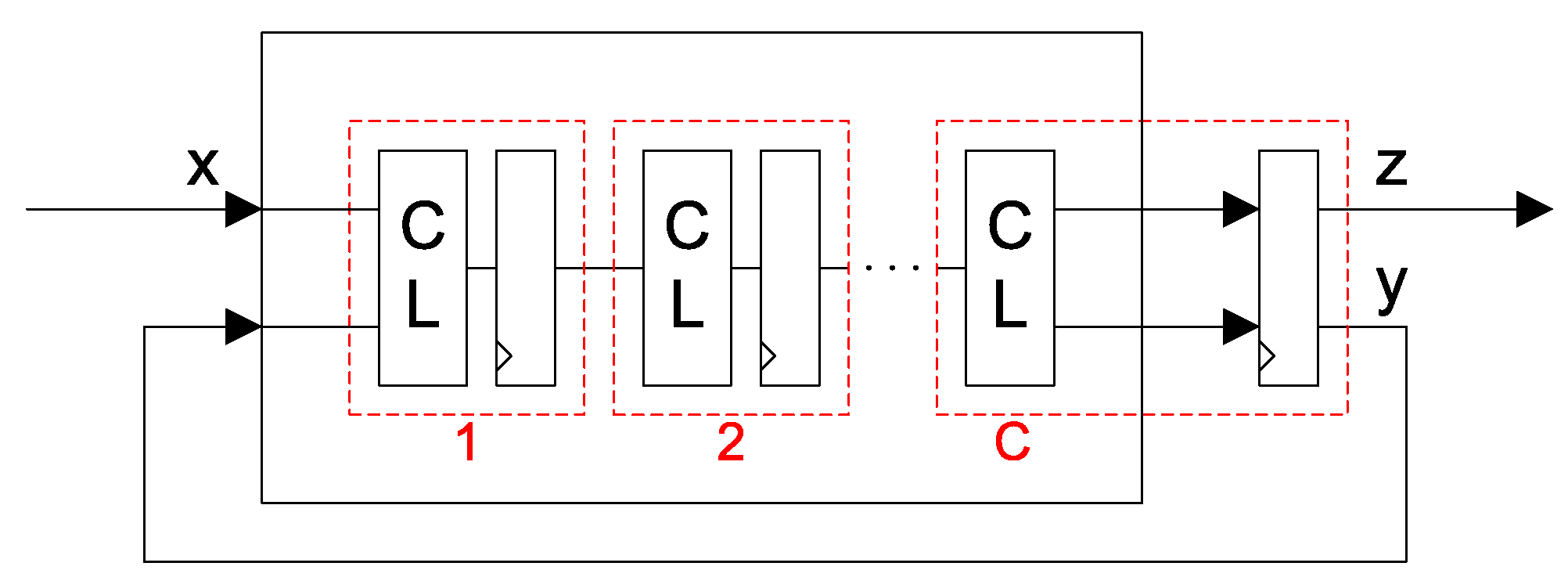
3.1. Virtual Hardware Configuration

Returning to Figure 1, when the logic function is purely combinational (i.e., feed-forward), any input from any data stream can be presented to the HW block at any clock cycle, even if it is deeply pipelined. In this case, there are no constraints on scheduling. When the logic function is sequential (i.e., has feedback) and has been deeply pipelined, this imposes scheduling constraints. Once a data element from a particular stream has been delivered to the HW block, the stream has to wait a number of clock ticks equal to the pipeline depth before it can provide a subsequent data element from that same stream.

Pipelined logic circuits with feedback can be context switched to compute multiple data streams concurrently. Essentially, the circuit can be thought of as a sequential logic circuit with pipelined combinational logic. The pipelined combinational logic adds latency and decreases single stream throughput since it takes multiple clock cycles (corresponding to the number of pipeline stages) to compute a single result and feed it back to the input. If the number of pipeline stages is C, then this circuit is said to be C-slowed since a single computation takes C times more clock cycles (often mitigated by a higher clock rate). Exploiting this characteristic allows processing multiple different contexts or data streams in a fine-grain way using the same hardware logic. The number of fine-grain contexts supported equals the pipeline depth.

When the number of contexts to be supported, N, is greater than the pipeline depth, C, coarse-grained context switching can be used, swapping out whatever state is stored in the circuit to a secondary memory. In general, this will incur some cost, representing the overhead of a context switch. While the fine-grained context switching of the C-slowed circuit naturally uses a round-robin schedule, there are a richer set of scheduling choices available when building a coarse-grain context switched design. In this work, we constrain our consideration to round-robin schedules in the queueing model and explore the performance impact of the schedule period. This constraint is dropped in the logic simulation, and several alternate schedule algorithms are explored.

We consider a general virtualized hardware configuration in Figure 4 with fine- and coarse-grained context switching. An arbitrary sequential logic circuit (i.e., the HW block) is C-slowed and augmented with a secondary memory that can load and unload copies of the state to/from the “active” state register. N FIFO, or First In, First Out, buffers are present at the inputs to store data stream elements that are awaiting being scheduled. The circuit consumes one data element (from an individual input specified by the schedule) each clock tick.

We develop several models of this circuit to predict system performance that allow a hardware designer to tune the performance. Inputs to the model and model assumptions are described first. The number of input data streams is denoted by N. Each data stream, i, is assumed to provide elements with a known distribution and given mean arrival rate ${\lambda }_i\mathrm{elements}/\mathrm{s}$. To start, we will assume the input distribution is Poisson. We will also assume that both the secondary memory and input buffers operate at the clock rate of the pipeline, and that the input buffers are sized sufficiently large to assume infinite capacity. State transfers to/from secondary memory take a given S clock cycles (enabling the model to support a range of context switch overheads), and the input buffers are assumed to have single-cycle enqueue and dequeue capability (i.e, they do not limit the performance of the system).

With the above model inputs provided, we represent the performance of the context switched hardware via the open queueing network illustrated in Figure 5. Each individual queueing station represents oual copy of the hardware computation. The arrival rate at each queue is ${\lambda }_i\mathrm{elements}/\mathrm{s}$, and the service distribution is described below.

3.2. M/G/1 Model Development

We develop a model of the system with an independent M/G/1 queueing station where the server can go on vacation for some time. In this model, the service distribution is general and, during a vacation, the server is not servicing any of its queued data elements. Here, we employ a round-robin schedule. In simulation, we will expand the set of schedules investigated.

Referring to Figure 5, the system consists of N queueing stations which all share a single physical server which is represented as being N “virtual” servers. We employ a fixed, hierarchical, round-robin schedule. Initially, a set of C input streams share the hardware resource and execute in a round-robin fashion in the server (in the computation pipeline). After $R_S$ rounds, the current set of C input streams’ state is swapped out (context switched) to secondary memory with cost S and the next set is swapped in. The collection of input stream sets are also context switched in a round-robin fashion.

The hierarchical nature of the schedule (i.e., fine-grained, round-robin schedule of contexts plus coarse-grained, round-robin schedule of groups of contexts) results in two types of vacations in the queueing model: short and long. Short vacations are due to fine-grain context switching and are only taken when the server is idle (i.e., the FIFO queue is empty). They occur because arrivals to a non-empty queue are aligned with the fine-grained schedule by the current entry in service. They last for C clock cycles. Long vacations are due to coarse-grain context switching and are taken when the schedule has completed $R_S$ rounds of the current set of C input streams and context switches to execute the other $N-C$ input streams, according to the fixed schedule. They occur for the duration of the vacation period. During these times, no new elements are processed until the vacation completes.

A single queueing station of the system, shown in Figure 6, consists of a FIFO queue and “virtual” server. $W_q$ is the mean waiting time in the queue and $W_s$ is the time spent in the server. When the server takes a vacation, this produces an additional waiting time at the head of the queue. We can derive a vacation waiting time, V, that is used in the calculation of $W_q$. It is modeled with a distribution determined by the fixed, hierarchical, round-robin schedule and is defined next. $W_s$ is modeled by a fixed service time X.

3.2.1. Vacation Waiting Time Model

To model the vacation waiting time, V, we define two sub-model distributions: $V_e$ for an empty queue shown in Figure 7a, and $V_n$ for a non-empty queue shown in Figure 7b. For the case of an empty queue, the probability density function, $f_{V_e}\left(v_e\right)$ shows the distribution of the vacation waiting time for continuous random variable $V_e$. $T_V$ is the time in a long vacation period (i.e., during a coarse-grain context switch), $p_s$ is the fraction of time in a service period, and $p_v$ is the fraction of time in the long vacation period. Along the x-axis, $v_e$ is measured in time and normalized to clock cycles, where $t_{CLK}$ is the clock period.

We start the model by defining the total number of clock cycles to complete a full round of the hierarchical schedule as

$$T_T=R_{S}N+SN/C.$$

(1)

The number of clock cycles in a long vacation period, which is the time during which the server has context switched to process other contexts, is

$$T_V=R_S\left(N-C\right)+SN/C.$$

(2)

The fraction of time in a service period is

$$p_s=R_{S}C/T_T,$$

(3)

and the fraction of time in a long vacation period is

$$p_v=1-R_{S}C/T_T.$$

(4)

The probability density function, $f_{V_e}\left(v_e\right)$, in Figure 7a, consists of two stacked rectangles with areas $p_s$ and $p_v$ whose sums must equal 1. Therefore, we can define $f_{V_e}\left(v_e\right)$ to be

$$\begin{array}{cc}{f}_{V_e}\left(v_e\right)\hfill & =\left(\frac{1-p_s}{T_V·t_{CLK}}\right)·\left[u\left(v_e\right)-u\left(v_e-T_V·t_{CLK}\right)\right]\hfill \\ & \hspace{1em}+\left(\frac{p_s}{C·t_{CLK}}\right)\left[u\left(v_e\right)-u\left(v_e-C·t_{CLK}\right)\right]\hfill \end{array}$$

(5)

where

$$u\left(x\right)=\left\{\begin{array}{cc}0\hfill & x<0,\hfill \\ 1\hfill & x\ge 0.\hfill \end{array}\right.$$

Next, for the case of a non-empty queue, the probability density function, $f_{V_n}\left(v_n\right)$, in Figure 7b, shows the distribution of the vacation waiting time for continuous random variable $V_n$. In this figure, the impulses defined at 0 and $T_V·t_{CLK}$ are Dirac delta functions ($\delta \left(x\right)$ notation) where

$$\begin{array}{cc}\hfill d_{ϵ}\left(x\right)& = \left\{\begin{array}{cc}1/ϵ\hfill & -ϵ/2\le x\le ϵ/2,\hfill \\ 0\hfill & otherwise,\hfill \end{array}\right.\hfill \\ \hfill \delta \left(x\right)& = \underset{ϵ\to 0}{lim}{d}_{ϵ}\left(x\right),\hfill \end{array}$$

and ${\int }_{-\infty }^{\infty }\delta \left(x\right)dx=1$. Along the x-axis, $v_n$ is measured in time and normalized to clock cycles.

Here, the two impulses define the vacation waiting time (and are normalized to the total number of jobs, $R_S$, in a full round of the hierarchical schedule). The first impulse, at $v_n=0$ (i.e., no wait time), defines a group of $R_S-1$ jobs being serviced consecutively. When these jobs complete, the server goes on a long vacation, and the next job waits for the vacation to complete. The wait time of the one job is then modeled by the second impulse, at $v_n=T_V·t_{CLK}$.

The probability density function, $f_{V_n}\left(v_n\right)$, is then

$$f_{V_n}\left(v_n\right)=\frac{R_S-1}{R_S}\delta \left(v_n\right) + \frac{1}{R_S}\delta \left(v_n-T_V·t_{CLK}\right).$$

(6)

Since the queueing station is using the fixed, hierarchical schedule, the probability of the queue being empty changes depending on whether the server is in a service or vacation period. Although it might change, we will assume that this probability is fixed for the purposes of combining the probability density functions, $f_{V_e}\left(v_e\right)$ and $f_{V_n}\left(v_n\right)$, into a single approximate function, $f_V\left(v\right)$. When we do this, we get

$$\begin{array}{cc}\hfill f_V\left(v\right)& =p_0·f_{V_e}\left(v\right) + \left(1-p_0\right)·f_{V_n}\left(v\right)\hfill \\ & =p_0·\left[\frac{1-p_s}{T_V·t_{CLK}}\left[u\left(v\right)-u\left(v-T_V·t_{CLK}\right)\right]\right.\hfill \\ & \hspace{1em}+ \left.\frac{p_s}{C·t_{CLK}}\left[u\left(v\right)-u\left(v-C·t_{CLK}\right)\right]\right]\hfill \\ & \hspace{1em}+ \left(1-p_0\right)·\left[\frac{R_S-1}{R_S}\delta \left(v\right)+\frac{1}{R_S}\delta \left(v-T_V·t_{CLK}\right)\right]\hfill \end{array}$$

(7)

where $p_0=1-\rho$, the probability of an empty queue.

Calculating the expected value, $E\left[V\right]$, of the vacation waiting time to get the mean vacation waiting time, we get the following:

$$\begin{array}{cc}\hfill E\left[V\right]& ={\int }_{-\infty }^{\infty }v·f_V\left(v\right)dv\hfill \\ & =\left[\frac{1}{2}{p}_0·\left[\left(1-p_s\right)·T_V+p_s·C\right]+\left(1-p_0\right)·\left[\frac{T_V}{R_S}\right]\right]·t_{CLK}\hfill \end{array}$$

(8)

The mean vacation waiting time will be denoted as $\overline{V}$ when used in the derivation of the queueing model equations.

3.2.2. Service Time Model

The model for the service time, X, is fixed and deterministic. For every job that enters the computational pipeline, it always takes exactly C clock cycles to complete service of that job. Therefore, the service time can be modeled as a single impulse function at $x=C·t_{CLK}$. The resulting probability density function, $f_X\left(x\right)$, is

$$f_X\left(x\right) = \delta \left(x-C·t_{CLK}\right).$$

(9)

Next, we can calculate $E\left[X\right]$, the expected service time, as

$$E\left[X\right] ={\int }_{-\infty }^{\infty }x·f_X\left(x\right)dx=C·t_{CLK}.$$

(10)

As part of the queueing model, we also need to know the second moment of the service time, $E\left[X^2\right]$. This is

$$E\left[X^2\right] ={\int }_{-\infty }^{\infty }{x}^2{f}_X\left(x\right)dx=C^2·t_{CLK}^2.$$

(11)

We will denote $E\left[X\right]$ as $\overline{X}$ and $E\left[X^2\right]$ as $\overline{X^2}$ in the development of the queueing model equations that follow.

3.2.3. Queueing Model

First, we start by defining the (deterministic) time in the pipelined circuit as

$$W_s=\overline{X}=C·t_{CLK}.$$

(12)

The effective service rate, ${\mu }_s$, of a “virtual” server is not equal to $1/W_s$, but has to take into account the long vacation time due to a coarse-grain context switch. We can do this by defining the service rate as the number of jobs processed by a stream in one full period of the hierarchical schedule. Therefore, for this M/G/1 system, the service rate, which is also the maximum achievable throughput (per stream), is

$${\mu }_s=\frac{R_S}{\left(R_{S}N+SN/C\right)·t_{CLK}}.$$

(13)

The total achievable throughput is then $T_{TOT}=N·{\mu }_s$, or

$$T_{TOT}=\frac{R_S}{(R_S+S/C)·t_{CLK}}.$$

(14)

The queuing system is stable when $\rho <1$ where $\rho =\lambda /{\mu }_s$ and $\lambda$ is the mean arrival rate. Using this criteria, we can solve for the minimum schedule period, $R_S$, for a stable system as

$$R_S>\frac{SN\lambda t_{CLK}}{C\left(1-N\lambda t_{CLK}\right)}.$$

(15)

The actual minimum $R_S$ is the next integer above the calculated value. Applying the floor function and adding 1, the minimum $R_S$ is then

$$R_{S,min}=1+⌊\frac{SN\lambda t_{CLK}}{C\left(1-N\lambda t_{CLK}\right)}⌋.$$

(16)

The average (mean) waiting time of each data element for an M/G/1 system (without vacations) is determined by the Pollaczek-Khinchin (P-K) formula as $W_q=\frac{\lambda \overline{X^2}}{2\left(1-\rho \right)}$ where $\overline{X^2}$ is the second moment of the service time (again, without vacations) [22]. To account for vacations, we need to add an additional waiting time at the head of the queue. For this, we use Equation 3.46 in [22] of the P-K formula derivation which uses a mean residual time, R, to solve for the wait time in the queue. The wait time formula then becomes $W_q=R+\frac{1}{{\mu }_s}{N}_q$ where $R=\frac{1}{2}\lambda \overline{X^2}$ and $N_q=\lambda W_q$ (Little’s Law [25]). Now, we can add the mean vacation waiting time, $\overline{V}$, to $W_q$ and apply Little’s Law:

$$W_q=R+\frac{1}{{\mu }_s}\lambda W_q+\overline{V}.$$

Solving for $W_q$ then gives

$$W_q=\frac{R+\overline{V}}{1-\rho }=\frac{\lambda \overline{X^2}}{2\left(1-\rho \right)}+\frac{\overline{V}}{1-\rho }.$$

(17)

Next, the average latency (elapsed time from arrival to completion of processing; we assume one output is generated per input) for each data element is

$$\begin{array}{cc}\hfill W_T& =W_q+W_s=\frac{\lambda \overline{X^2}}{2\left(1-\rho \right)}+\frac{\overline{V}}{1-\rho }+\overline{X}\hfill \\ & =\left[\frac{C^2\left(\lambda ·t_{CLK}\right)}{2\left(1-\rho \right)}+\frac{1}{2}\left[\left(1-p_s\right)·T_V+p_s·C\right]+\frac{\rho }{1-\rho }·\left[\frac{T_V}{R_S}\right]+C\right]·t_{CLK}.\hfill \end{array}$$

(18)

The average (mean) occupancy of each queue is $N_q=\lambda W_q$.

The expression for the average latency consists of 5 terms that model the delay through the system. The first term ($\frac{\lambda C^2{t}_{CLK}^2}{2\left(1-\rho \right)}$) models service queueing delay. The second term ($\frac{1}{2}\left(1-p_s\right)T_V·t_{CLK}$) models long vacation delay during a vacation period. The third term ($\frac{1}{2}{p}_s·C·t_{CLK}$) models short vacation delay during a service period for an empty queue. The fourth term ($\frac{\rho }{1-\rho }\frac{T_V·t_{CLK}}{R_S}$) models vacation queueing delay. Furthermore, the fifth term ($C·t_{CLK}$) models service time delay. Of these delays, those due to the long vacation period (the second and fourth terms) have the greatest impact on the average latency. The vacation queueing delay (fourth term) accounts for large initial latency at low $R_S$ due to the effect of S, but decreases when $R_S$ increases (by amortizing the effect of S). The long vacation delay (second term) accounts for a gradual increase in latency with increasing $R_S$ since $T_V$ increases with $R_S$.

To summarize the queueing model notation used in the derivation above,

Table 1. Queueing model notation.

Term	Label	Term	Label
N	Number of data streams	$T_V$	Vacation time
C	Pipeline depth	$p_s$	Service time fraction
S	Context switch cost	$\overline{V}$	Mean vacation waiting time
$R_S$	Schedule period	$\overline{X}$	Mean service time
$t_{CLK}$	Clock period	$\overline{X^2}$	Service time second moment
$T_T$	Total schedule time	$T_{TOT}$	Total achievable throughput

lists the notation in abbreviated form.

3.3. Simulation Models

To both validate the queueing model formulated above and expand the scope of the performance evaluation, we developed a pair of simulation models. The first of these is a discrete-event simulation model authored in Python, and the second is a detailed design of some components authored in VHDL. One motivation for these multiple models is to provide a spectrum of abstractions: an analytic model, a discrete-event simulation model with a continuous-time arrival process, and a detailed design that has a full implementation of several components that are abstracted in both the analytic and discrete-event simulation models.

3.3.1. Discrete-Event Simulation

We designed and implemented a cycle-accurate discrete-event simulation of the virtualized hardware design from Figure 4 using the SimPy discrete-event simulation framework [26] written in Python. The simulation system is illustrated in Figure 8. It consists of arrival processes, a scheduler, and virtual computation processes. The arrival processes are continuous-time, and the server, composed of the scheduler and virtual computation processes, is discrete-time, cycle-accurate. Statistics are gathered in each of these processes to track the jobs in the system. Startup transients are removed from the statistics collection.

There are N arrival processes, one for each input queue that represents a virtual computation. Jobs arrive into the system with an interarrival time computed based on a given distribution (e.g., exponential, Erlang, hyperexponential, etc.). When a job arrives, it is put into the input queue. The server, composed of the scheduler and virtual computation processes, emulates the hardware design in Figure 4. Each input queue is visited according to the hierarchical round-robin scheduler described above in Section 3.2, taking one clock cycle or $t_{CLK}$ time per visit and $S·t_{CLK}$ time per context switch.

Going back to the input queue, the server checks for an available job. If a job is available, it is removed from the queue and begins service. Service begins by starting a new virtual computation process that simulates processing the job in the C pipeline stages of the hardware by delaying $C·t_{CLK}$ time. When it is done, the job completes service. Going back to the input queue, if a job is not available, then no virtual computation process is started. This simulates a gap or unused pipeline stage in the real hardware design.

We will use this discrete-event simulation model for two purposes: first to validate the queueing model, and second to explore the performance impact of alternate arrival distributions.

3.3.2. Logic Simulation

To enable the investigation of multiple scheduling algorithms, we coded a test system in VHDL that includes a simple pipeline augmented with a full implementation of the input queues, input multiplexers, and secondary memory of Figure 4. It also includes the control logic for the data path, which specifies the scheduling algorithm. Figure 9 illustrates this design.

In this design, the secondary memory is implemented in a way that is appropriate when the total number of contexts, N, is not substantially larger than the pipeline depth, C. Here, we demultiplex the next state information output from the Cth stage of the combinational logic and save it in N registers (one per context). The scheduler selects a (potentially different) context for feedback into the front end of the pipeline. In this circumstance, the overhead for a coarse-grain context switch, S, is eliminated (i.e., $S=0$). Note, there are circumstances for which a zero-overhead context switch would be unreasonable, for example, when the number of contexts is significantly larger than the pipeline depth or when the quantity of state information is large (e.g., an imaging application).

There are three distinct controller designs, each of which implements a different scheduling algorithm. The first is the hierarchical round-robin schedule that is present in the analytic and discrete-event simulation models. The implementation is straightforward, with the next input queue to select being simply the next one in line. While well suited to analysis, this schedule will clearly be not work-conserving, in the sense that it is possible to have non-empty queues in the system yet the schedule will choose an empty queue to service in a specific time slot.

The second scheduling algorithm, while still technically not work-conserving, is an attempt to retain the simplicity of the implementation of the round-robin schedule yet diminish the frequency with which empty queues get scheduled. This is accomplished by checking the occupancy of the next input queue, and if it is empty skipping it and moving ahead to the next queue.

The third scheduling algorithm examines the occupancy of all of the queues and selects the queue with the maximum occupancy for the next time slot. This schedule is clearly work-conserving, but has the highest complexity of each of the scheduling algorithms.

Since the implementation is in VHDL, we are able to use the tools to perform logic simulation on these designs. With the VHDL implementation of Figure 9, we are interested in investigating a number of issues:

• The specifics of the secondary memory are left unspecified in Figure 4.
• In the analytic and discrete-event simulation models, we assume that neither the input queueing and multiplexer data path nor the scheduler and other control logic limit the operating clock frequency of the system.
• The only scheduling algorithm investigated so far is a hierarchical round-robin algorithm.

We discuss the first of these below, and defer the discussion of the other to later sections.

In Figure 4, the specifics of the secondary memory design are left completely generic (i.e., unspecified), and the overhead associated with a coarse-grained context switch, S, is an input to the performance models. This has the benefit of being quite general, in the sense that many possible designs for the secondary memory can be readily incorporated into the models, making the models amenable to use with applications that have widely varying state requirements.

For the logic simulation, it is incumbent upon us to choose a specific secondary memory design, and the design of Figure 9 is appropriate for applications with small state requirements for each context. In a sense, the secondary memory is actually being implemented as simply a larger number of primary state registers. To justify the conclusion that the context switch overhead, S, is zero for this design, we must verify that the demultiplexer, registers, and multiplexer in the feedback path (providing signal y in Figure 9) do not limit the achievable clock frequency of the system. This verification is discussed as part of the investigation of the above point (2) in Section 3.5 below.

3.4. Clock Model

The service rate of each virtualized server is a function of the underlying clock period. The clock period, however, is impacted by the degree to which a circuit has been C-slowed. Here, we describe an approach to modeling this relationship.

A C-slowed circuit, shown in Figure 10, consists of a sequential logic circuit (i.e., a circuit with combinational logic and a feedback path) that is pipelined with C pipeline stages. The pipeline stages are to be distributed evenly throughout the combinational logic and we model the stage-to-stage delay using a random variable. If $t_{CL}$ is the total combinational logic delay for a non-pipelined circuit, then the mean stage-to-stage combinational logic delay will be $t_{CL}/C$. There is variation in the stage-to-stage delay due to the placement of logic and the routing of signals between logic, which we model stochastically. The clock period, $t_{CLK}$, is then determined by the worst-case logic path, which is the maximum stage-to-stage delay in the C-slowed circuit. Therefore, we can model $t_{CLK}$ as the expectation of the maximum of C samples of a random variable D where D is the stage-to-stage delay.

The model for $t_{CLK}$, developed fully in [27], is

$$t_{CLK}\left(C\right)=\frac{k_1}{C}+k_2·{\left(lnC\right)}^{0.7}.$$

(19)

This is a reasonable model that allows us to calibrate the clock period from FPGA synthesis results below in Appendix A and use in the performance models to make predictions below in Section 4. Here, C is the number of pipeline stages, and $k_1$ and $k_2$ are curve-fit parameters of the model. $k_1$ represents the curve-fit total combinational logic delay of the circuit (which should be approximately equal to $t_{CL}$), so that as C increases, $k_1/C$ decreases. $k_1/C$ is the mean stage-to-stage delay for combinational logic that is evenly pipelined with C pipeline stages.

3.5. Model Validation

The validation of the various models will take a pair of forms. First, we will use the VHDL implementation of the logic simulation to verify the correctness of some modeling assumptions made as part of the queueing model and the discrete-event simulation model. Second, we will use all three models to do an empirical cross-validation, making performance predictions at common design points and ensuring that the performance predictions are compatible with one another.

3.5.1. Verifying Assumptions

In the model for $t_{CLK}$ developed above and used in both the queueing model and the discrete-event model, the focus was entirely on the C-slowed data path of Figure 4. It was explicitly assumed that the input queues, input multiplexer, secondary memory, output multiplexer, and control logic would not be limiting factors in the clock frequency. We synthesized the VHDL design of Figure 9, which includes all of these elements, to test this assumption. For the first two scheduling algorithms, the achievable clock rate is (to first order) independent of the number of inputs and outputs, and the synthesized VHDL design clocks faster than any of the calibrated clock frequencies presented in Appendix A below (over 500 MHz).

For the third scheduling algorithm, in which one needs to determine the maximum queue occupancy over all the inputs, our VHDL implementation uses a simple linear comparison technique, which clearly will be strongly dependent on the count of inputs and outputs. The performance predictions below in Section 4 are made with $N=8$ inputs, and for this case, the achievable clock frequency ($172.1 \mathrm{MHz}$) is greater than the $t_{CLK}$ predicted by (19) ($168.8 \mathrm{MHz}$ for SHA-256). For larger numbers of inputs, however, it would be necessary to alter the implementation of the scheduler to be more efficient (e.g., use logarithmic time complexity approaches to determine which queue has maximum occupancy).

3.5.2. Cross-Validation of Performance Models

The cross-validation compares the analytic queueing model to each of the two simulation models at different points in the design space. For the logic simulation, the implementation of Figure 9 ($C=4$, $N=8$, $S=0$) is simulated with Poisson-distributed arrivals providing an offered load of $OL=0.5$. The performance figure of interest is mean queue occupancy (which can be related to latency, or time in the system, by Little’s Law [25]). Ten repetitions are executed, with the first 20% of the statistics discarded to eliminate startup transients. The result of the experiment was a mean queue occupancy of $0.408\pm 0.033$ at 99% confidence level. This compares favorably to the analytical model result for mean queue occupancy ($N_q$) of 0.438, well within the confidence interval. For visual reference, this point is included on the graph in Section 4.4.

While the logic simulation is limited in the scope of input parameters that it supports, the discrete-event simulation is capable of modeling a much wider range of the design space. In this case, we directly measure the average latency of data elements from when they enter the input queue to when they exit the system. The workload is generated probabilistically with Poisson arrivals and the performance is measured at steady state. Each context is simulated with the same arrival distribution and rate (but different random streams). Since the virtualized hardware uses a round-robin schedule, each context is independent and can be treated as an ensemble of M/G/1 queues that can be averaged together. Consider a candidate design with 10 fine-grained contexts ($C=10)$, 100 total contexts ($N=100$), and a 100 clock overhead to perform a coarse-grained context switch ($S=100$). Figure 11a plots the total latency ($W_T$) predicted by (18) vs. the schedule period ($R_S$), for an offered load of $0.08$ and $0.5$. The points on the graph correspond to empirical results from the discrete-event simulation run with the same parameters and averaged over the ensemble of M/G/1 queues across the 100 contexts. As before, the offered load is defined as the ratio of the aggregate arrival rate (of all streams) to the peak service rate of the system (i.e., when $S=0$). Offered load then evaluates to $N·\lambda ·t_{CLK}$. We draw two conclusions from this figure. First, there is good correspondence between the analytical model and the empirical simulation results. This bolsters our confidence that the analytic model is reasonable. The small discrepancy that is present is likely due to the assumptions made in (7). Second, there is a schedule period that optimally minimizes latency for a given offered load. At an offered load of $0.08$, minimum latency is experienced with schedule period $R_S=3$. At an offered load of $0.5$, it is $R_S=15$. With the higher offered load, the system is not stable until $R_S\ge 11$, which is predicted by (16).

Additional validation was performed for a second candidate design with input values $C=4$, $N=8$, $S=4$, and $OL=0.16$ and $0.48$ and is shown in Figure 11b. Results are averaged across an ensemble of 10 replications of 8 contexts each (or 80 total samples). These results obtained also have good correspondence between the analytical model and simulation and the existence of a schedule period that minimizes latency.

3.6. Example Applications

We use three applications to illustrate use of the performance models. Here, we describe each application, and then below in Section 4, we use these same three applications to exercise all three performance models.

The three applications, listed in

Table 2. Applications implemented using C-slow techniques.

Abbr.	Name	Description
COS	Cosine application	Synthetic cosine application implemented via a Taylor series expansion with added feedback
AES	AES application	Advanced Encryption Standard (AES) cipher in cipher-block chaining (CBC) mode for encryption
SHA	SHA-2 application	Secure Hash Algorithm (SHA-2) with 256 and 512 bit digests (SHA-256 and SHA-512)

, are a synthetic cosine application implemented via a Taylor series expansion with added feedback, the Advanced Encryption Standard (AES) cipher in cipher-block chaining (CBC) mode for encryption, and the Secure Hash Algorithm (SHA-2) with 256 and 512 bit digests (SHA-256 and SHA-512). These applications were chosen because they each have a long combinational logic path with feedback from output to input, thus making simple pipelining alone insufficient to effectively utilize their logic blocks. This makes them good candidates for C-slow (pipelining) with virtualization where independent streams are scheduled for execution in the pipeline stages.

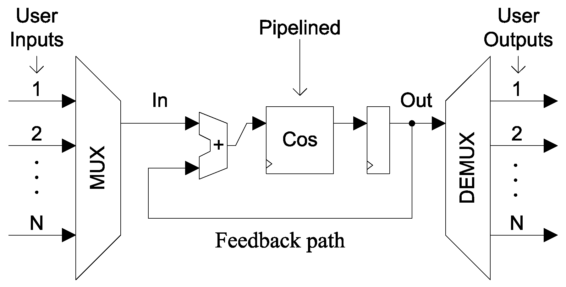
3.6.1. Synthetic Cosine Application with Added Feedback (COS)

The Cosine application, illustrated in Figure 12, consists of a cosine function, an output register, a feedback path, and an adder to mix the input with the output feedback. This is a synthetic application built to have a long combinational logic path through the cosine function via a configurable number of Taylor series terms, $N_t$, that approximate the cosine. The cosine function is pipelined with a configurable number of pipeline stages, C, to improve the clock period and to support C virtual streams of computation. This application is chosen to act in the role of a micro-benchmark. It is straightforward to understand and allows us to alter the salient properties that can impact performance (specifically the depth of the combinational logic path).

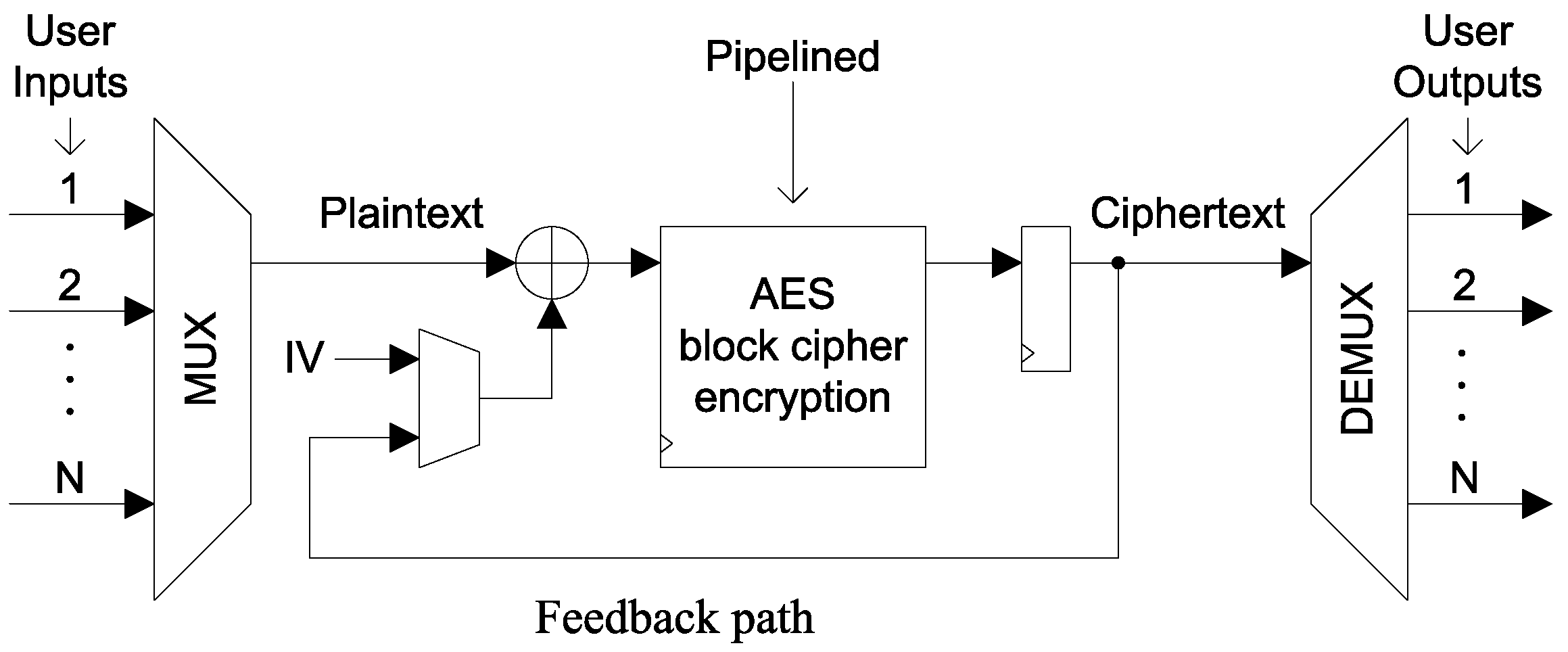
3.6.2. Advanced Encryption Standard (AES) Cipher in Cipher-Block Chaining Mode

Next, we use an AES encryption cipher [28] in CBC block mode (that has a feedback path) illustrated in Figure 13. In our implementation, the AES encryption cipher is fully unrolled forming a long combinational logic path with up to 14 rounds (the AES 256-bit standard), enabling us to investigate the impact of short vs. deep combinational logic functions. The number of rounds, $N_r$, in the cipher is configurable, which controls the length of the combinational logic. The AES block cipher is shown in the middle of the figure. Operating in cipher-block chaining (CBC) mode, an initialization vector (IV) is XOR’d with a plaintext block to produce the input to the cipher. The output is registered which contains the ciphertext output. The ciphertext is then fed back, through a multiplexer, to be mixed again with the next block of plaintext. The AES encryption cipher has a configurable number of pipeline stages, C, to improve the clock period and to support C virtual streams of computation. This is implemented via outer loop pipelining [29]. The AES encryption cipher has been chosen to be an example of a realistic computation that can be shared across applications within a multicore system. A hardware accelerated implementation can provide performance benefits over software implementations, and it is a function that is generally of use to many applications (e.g., it is one of the computations described in [8]).

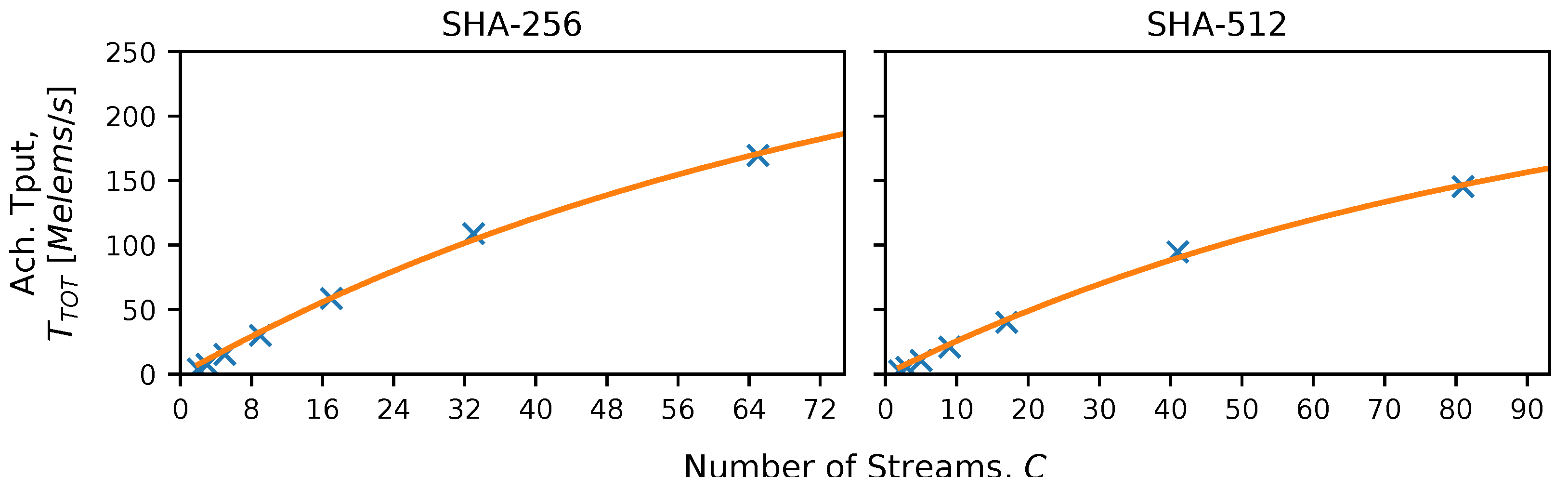
3.6.3. Secure Hash Algorithm (SHA-2) with 256 and 512 bit Digests

Last, we use an SHA-2 cryptographic hash application [30] (that has a feedback path for processing multiple blocks in a stream) illustrated in Figure 14. In our implementation, the SHA-2 core is fully unrolled forming a long combinational logic path with 64 rounds for SHA-256 and 80 rounds for SHA-512. The core is shown in the middle of the figure. To start, an initialization vector (IV) is provided with the first block of data to the input of the core (or hash function). The output is registered and eventually becomes the hash output after all data blocks have been processed. While processing each block, the intermediate hash values are fed back, through a multiplexer, to be mixed again with the next data block. The SHA-2 core has a configurable number of pipeline stages, C, to improve the clock period and to support C virtual computations at a time. The SHA-2 application is designed to compute on a single input stream containing arbitrary fields within record-oriented data that can be processed independently of each other. It uses a single stream interface that feeds an upfront content addressable queue (which serves the function of the input FIFOs in Figure 4). The queue buffers block data from each field which can be accessed at any position via a multiplexer. A reorder queue at the output reorders the field results back into their original order. The SHA-2 application is an example of a computation that could be deployed in a SaaS model, in which the hardware accelerated function is made available to users via the cloud.

4. Results and Discussion

We evaluate the use of virtualized logic computations with our analytical and simulation performance models. We predict performance given assumptions inherent in the analytical model (i.e., Poisson arrival process and hierarchical round-robin schedule) and evaluate those assumptions via simulation.

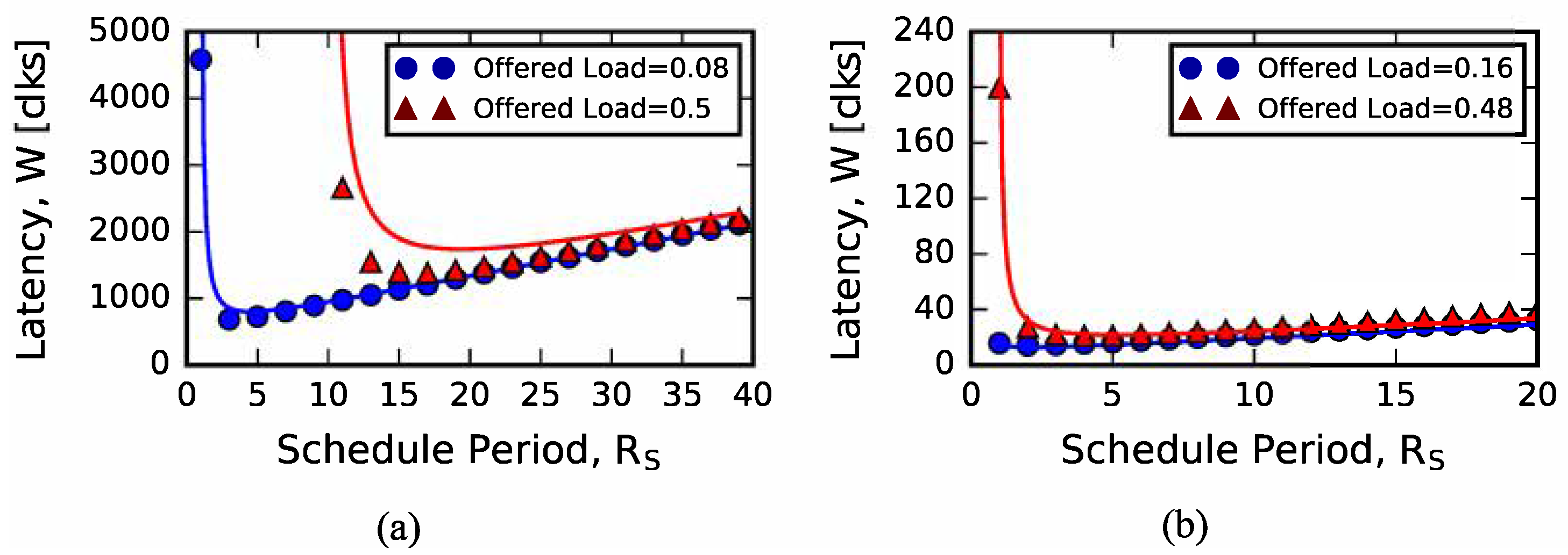
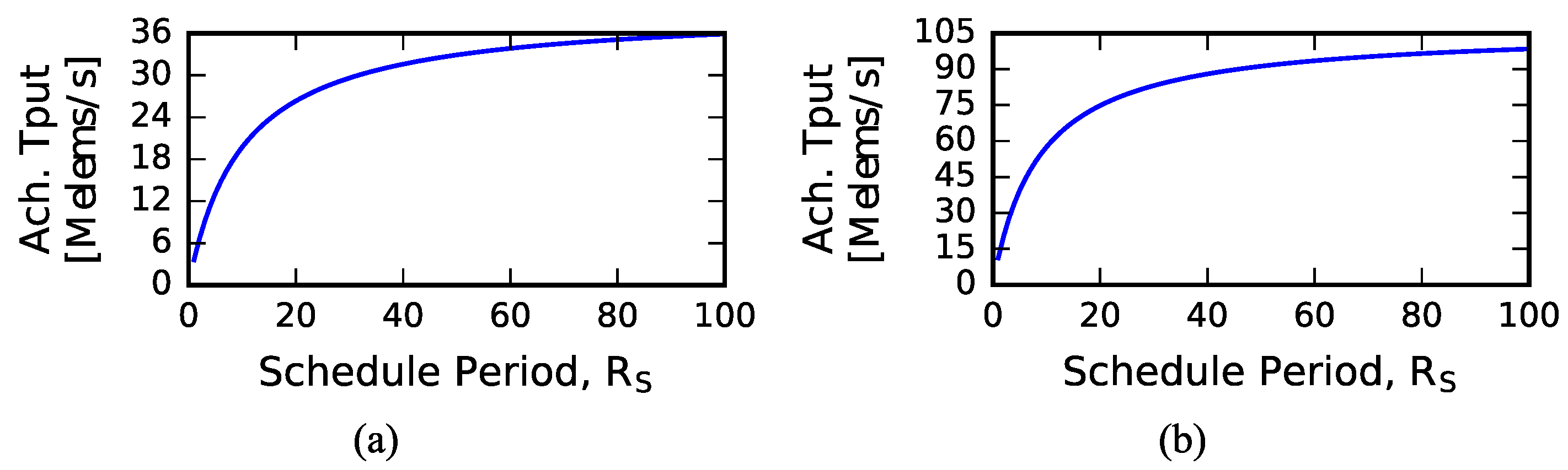
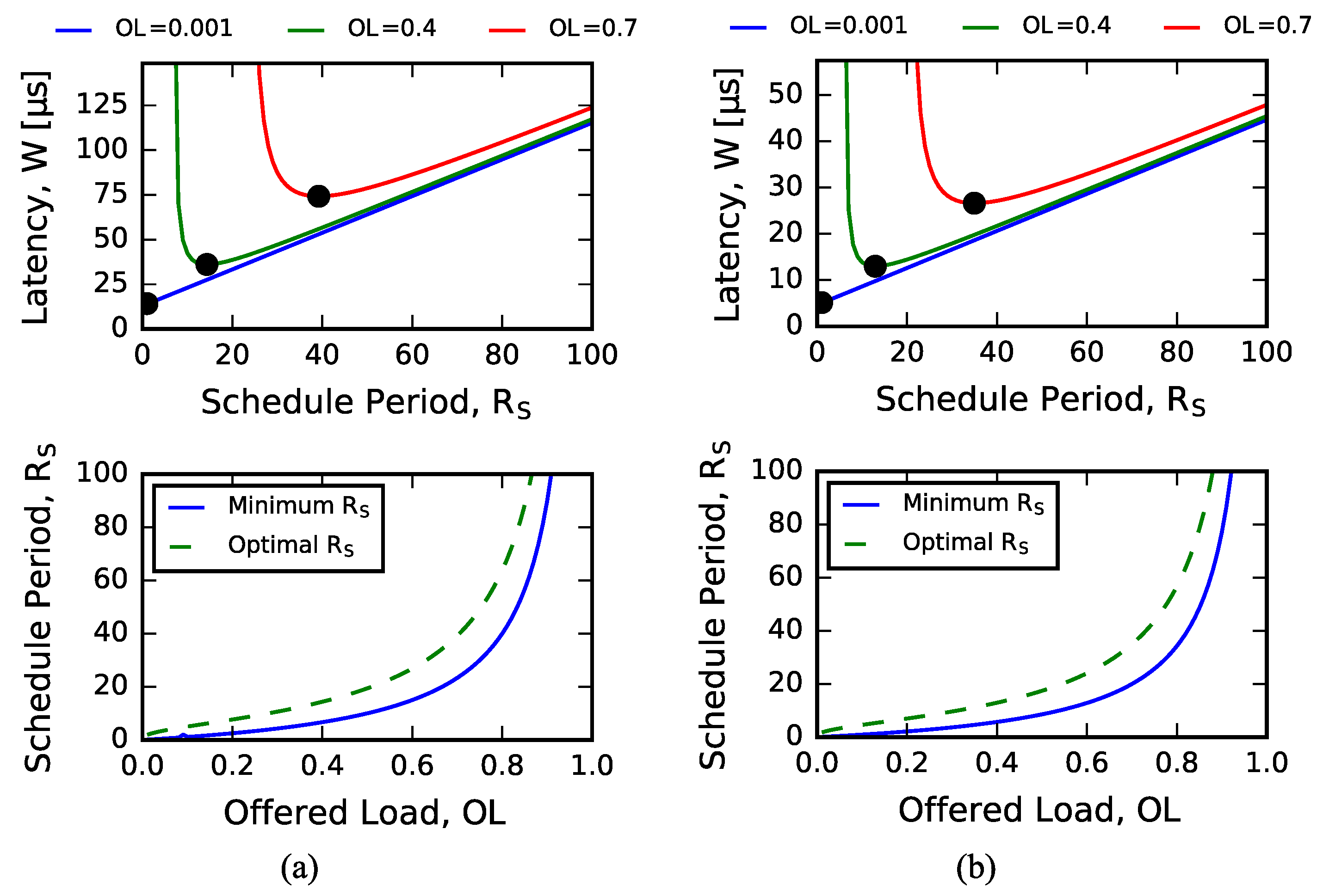
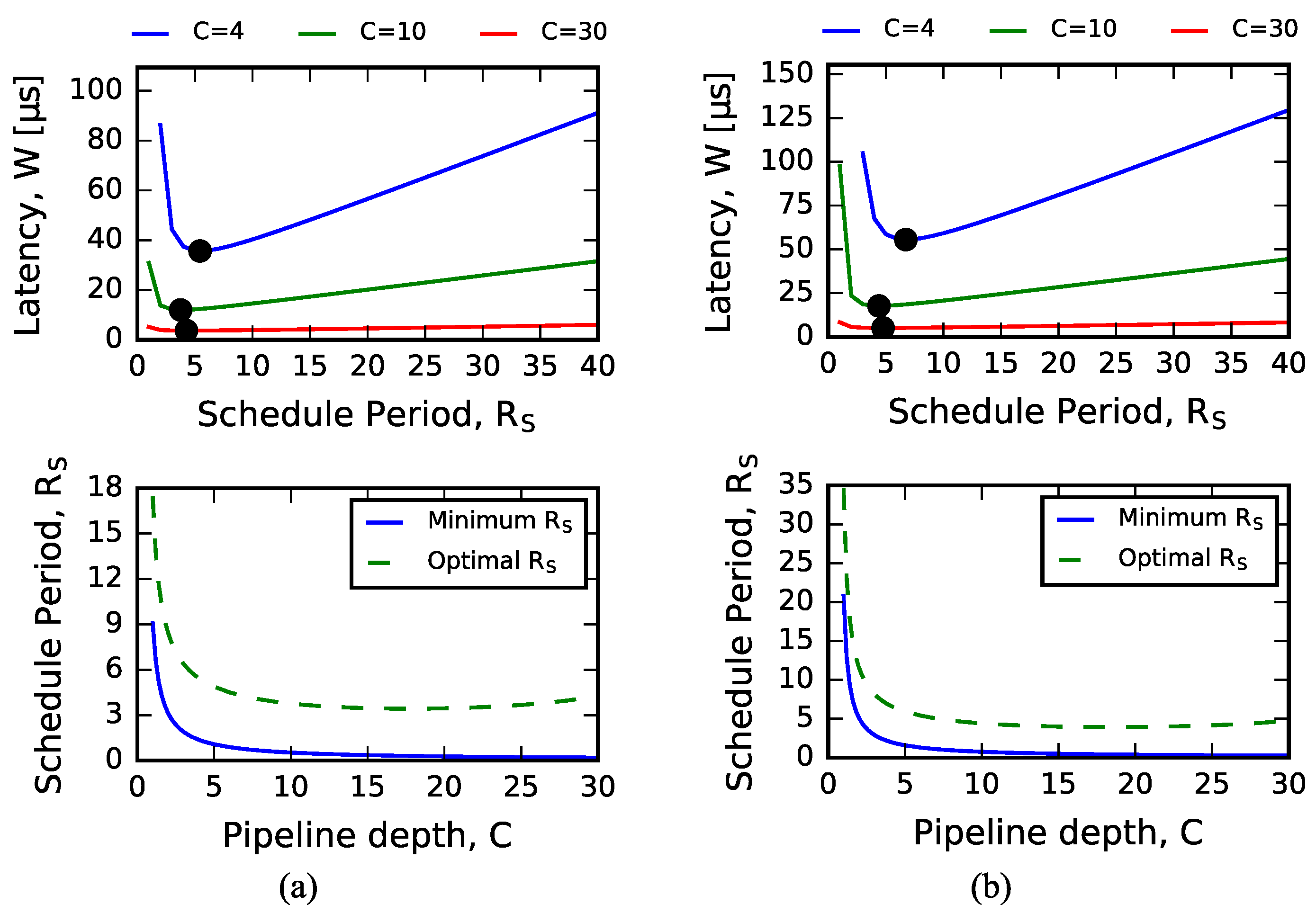
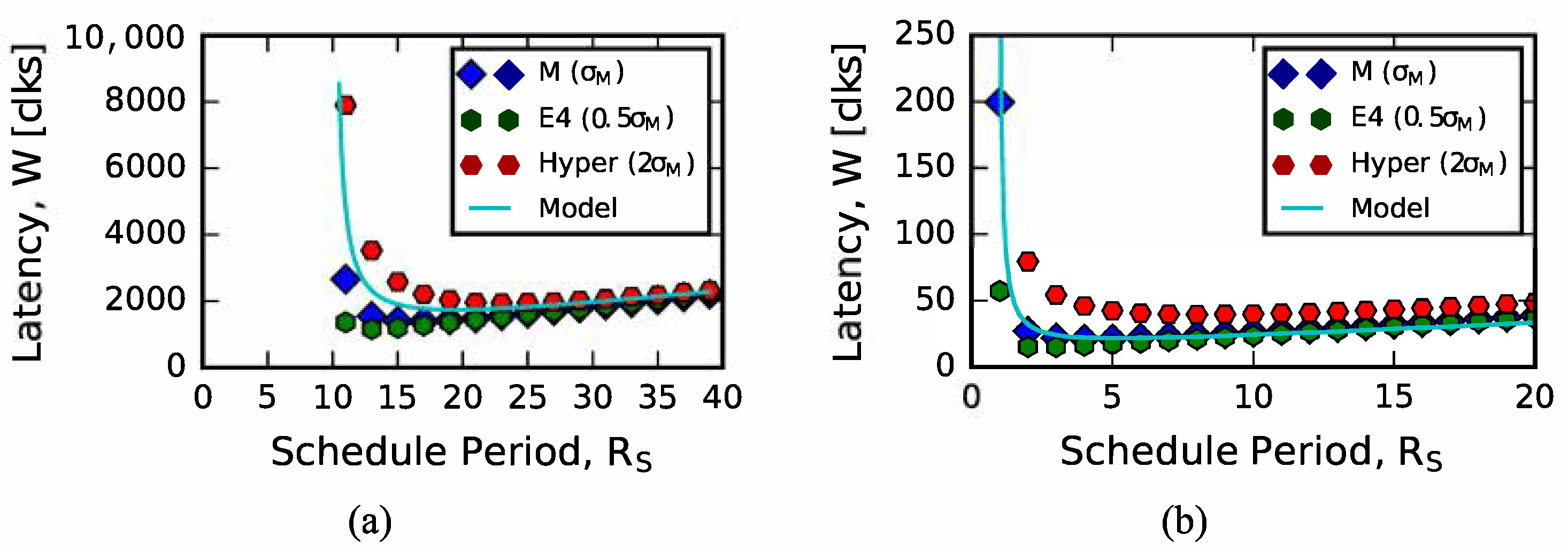
4.1. Analytical Model Predictions

We have application and technology independent M/G/1 queueing model equations developed above that can be used to predict the performance of virtualized logic computations for fine- and coarse-grain contexts. In this section, we show prediction results for COS, AES, and SHA-2 applications on FPGA technology. The use of the model on ASIC technology is described in [27].

The queueing model consists of inputs and outputs that make it flexible in predicting performance. For these results, we first focus on a specific design scenario. We are given a circuit, technology, the total number of contexts (N), the pipeline depth (C), and the cost of a context switch (S), and have a varying offered load ($OL$). We can tune the schedule period ($R_S$). We first present prediction results for total achievable throughput and latency. Then we optimize for minimum latency ($W_T$).

Total achievable throughput is shown in Figure 15a,b for the COS and AES applications. In these applications, one output is generated per input (i.e., in the case of AES, a block output is computed directly from a block input). As the schedule period ($R_S$) increases, the cost of a context switch (S) is amortized, resulting in higher total achievable throughput. The total achievable throughput depends on the clock period model in (A1) and (A2), and is a function of pipeline depth (C). Since C is fixed in this example, $t_{CLK}$ is constant and scales the plots.

The results for latency are shown in Figure 16a,b. The latency we are considering is the delay from data arriving at a stream input to the corresponding data being available at the stream output. In the figures, there are both latency and optimization plots. In the latency plots, the queueing model predicts mean latency ($W_T$) across a range of schedule periods ($R_S$) and three offered loads ($OL$). Offered load, as was previously defined, is the ratio of the aggregate arrival rate (of all streams) to the peak service rate of the system (i.e., when $S=0$). It evaluates to $N·\lambda ·t_{CLK}$.

Returning to the latency plot, there are three regions of interest. The first region is the high latency on the left which drops steeply. This high latency is due to traditional queueing delay, a normal consequence of high effective server utilization. The beginning of this region marks the minimum $R_S$ needed for a given offered load. Below this value, the context switch overhead is high enough that the provided offered load cannot be serviced, and the queueing system is unstable (i.e., grows to infinite queue length). As $R_S$ increases, total achievable throughput increases, causing queueing to decrease. The second region is at the knee of the curve. In this region, $R_S$ is optimal and gives minimum latency performance. The third region is to the right where latency gradually increases. This increase is due to the wait time incurred during a vacation period by the hierarchical, round-robin schedule as $R_S$ increases. It now takes longer for a data stream to be serviced. We can observe for an $OL=0.7$, the minimum latency is about 30 μs for AES.

In the optimization plots, latency is optimized across a range of offered loads swept from 0 to 1. There are two curves. The solid blue curve shows the minimum $R_S$ needed to service a given offered load (that is, $\rho <1$). The dashed green curve shows the optimal $R_S$ that minimizes latency at the given offered load. For AES, we can see that at low offered load, the optimal $R_S$ is small, then gradually increases until about 0.8, and finally increases steeply.

Comparing the COS and AES results qualitatively, we can see that they both produce the same shape of plots. The only real difference is the scale of the plots which is determined by the clock period model for each application.

Suppose we choose a value of $R_S$ from the optimization plot for the AES application. We can then plot the latency for this fixed $R_S$ versus the offered load to show a performance curve across all loads. This is shown in Figure 17 for three values of $R_S$. We can see that the latency is initially flat at low offered loads, but then increases steeply at some point. The “knee” of these curves, indicated by a black dot, is approximated to be 3 dB above the minimum latency of each curve. Beyond the knee, the latency increases sharply. As $R_S$ varies, the latency curve changes in two ways. First, it changes in the value of the latency in the flat part of the curve (low $R_S$ gives low latency). Second, it changes the position of the knee of the curve (high $R_S$ pushes the knee out further, allowing a large range of loads to be handled). This indicates a tradeoff. If we expect the load on the system to be small, we can sacrifice range of offered load to get low latency. Otherwise, we can sacrifice low latency for a large range. Optimizing $R_S$ continuously across all offered loads, we can attain the minimum latency for each offered load. This is shown as the dashed black curve, which establishes a lower bound on the latency.

The above results enable a user to dynamically tune the performance of a virtualized custom logic application in response to varying input load conditions. By adjusting the schedule period based on offered load, the system can be continuously operated in its minimum latency configuration.

Additional results are shown for the SHA-2 application. In these results, the pipeline depth (C) is varied along the x-axis. The clock period ($t_{CLK}$) given by (A3) and (A4) is a function of C, and will therefore affect the shape of the plots.

Total achievable throughput is shown in Figure 18a,b for SHA-256 and SHA-512. In the plots, $N=C$ and $S=0$ (i.e., no secondary memory). As the pipeline depth (C) increases, more data streams can be computed in parallel, and the clock period ($t_{CLK}$) decreases (initially linearly). This causes the total aggregate throughput of all data streams to increase initially linearly as well. As C gets higher, $t_{CLK}$ starts to flatten out, causing the throughput to bend over. The pipeline depth is swept up to the maximum number of pipeline stages, 65 in SHA-256 and 81 in SHA-512. Above these values of C, the total achievable throughput will be flat.

Latency prediction and optimization plots are shown in Figure 19a,b. In these results, N is fixed at 60 total streams, S is $10C$, and $\lambda =30 \frac{\mathrm{Kelems}}{\mathrm{s}}$. In the latency plots, three curves are shown for different values of the pipeline depth (C) and the schedule period ($R_S$) is swept along the x-axis. We can see the same three regions in the latency plots: initial high latency which drops steeply, an optimal minimal latency, and then a gradual increase in latency with increasing $R_S$. Of the three curves, we can see that the $C=30$ curve (with the highest C) has the lowest latency. This may be accounted for in part in that at high C, there are fewer context switches required.

In the optimization plots, there are two curves. The solid blue curve shows the minimum $R_S$ needed to service a given pipeline depth (that is, $\rho <1$). The dashed green curve shows the optimal $R_S$ that minimizes latency at the given pipeline depth. The pipeline depth ($R_S$) is swept along the x-axis. We can see that the optimal $R_S$ is mostly flat as C increases beyond about 5 in both SHA-256 and SHA-512.

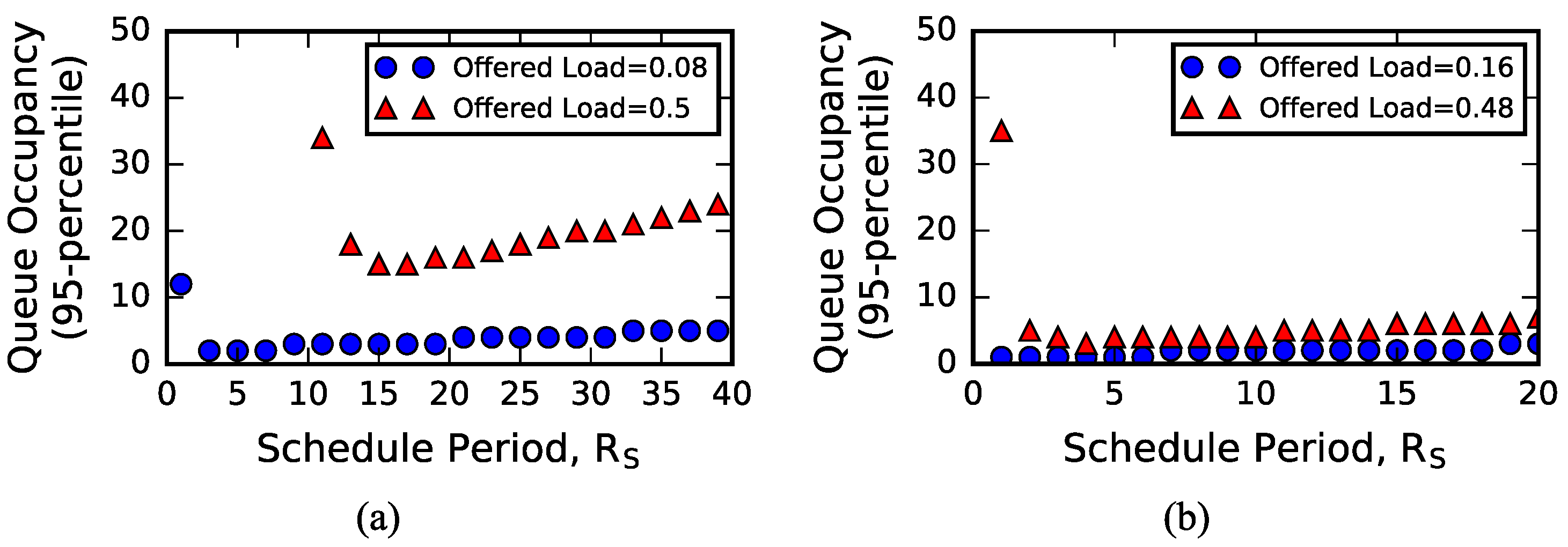
4.2. Sizing Input Queues

The size of the input queue needed for a virtual stream (i.e., the size of a FIFO in Figure 4) depends on the queue occupancy under load. Using the discrete-event simulation as described above, we measure the queue occupancy distribution and show the normalized histogram in Figure 20a,b for the two candidate designs under load with Poisson arrivals. We can estimate the size of the input queue by measuring percentiles. The 95th percentile is marked with a yellow vertical line and the 99th percentile is marked with a green vertical line. We make several observations. First, we observe that under load the probability distribution has a peak, which is clearly visible in the first candidate design. Second, the histogram shows an exponential decay in the probability with increasing jobs waiting in the queue. This causes a long tail. The 95th and 99th percentiles both estimate the queue occupancy but are shifted from each other. The 99th percentile includes more of the tail.

Using the 95th percentile, we show the queue occupancy of the two candidate designs in Figure 21a,b. We can see that the data points follow the same shape as that of the latency curve, which is consistent with Little’s Law [25] that relates latency, queue occupancy, and arrival rate.

Let us look more closely at the first design with 10 fine-grained contexts ($C=10$), 100 total contexts ($N=100$), and a 100 clock overhead to perform a coarse-grained context switch ($S=100$) to consider how to size the input queue. There are two things to consider in these results. The first is the queue occupancy at high $R_S$. (Note, as $R_S$ increases, the load on the system decreases because the cost of the coarse-grained context switch is being amortized. This decreases the contribution of the load to the queue occupancy.) To prevent backpressure during most of the normal usage of the system, the input queue size needs to be greater this value. The second is the queue occupancy at high load (i.e., high offered load and low $R_S$). This indicates the queueing that occurs on a loaded system. To reduce backpressure when under load, the input queue size needs to be above this value. For example, under load at $R_S=11$ and $OL=0.5$, the 95th percentile queue occupancy is 34. A designer might choose an input queue size of 40 or 50 to handle most loads with minimal or no backpressure.

4.3. Exploring Arrival Process Distribution

For some use cases (e.g., the SaaS model), a Poisson arrival process can be a very good match to what is observed in practice [31,32]. Clearly, for other use cases, the assumption of Poisson arrivals is not as realistic. Next, we explore the implications of the Poisson arrival process assumption, which has exponential interarrival times, by comparing it with other arrival distributions simulated by the discrete-event simulation described in Section 3.3.1. For this exploration, we simulate three interarrival distributions: exponential (M), Erlang (E4), and hyperexponential (Hyper). These distributions were chosen explicitly to explore circumstances with a narrower distribution than Poisson (the Erlang) as well as a wider distribution than Poisson (the hyperexponential). The exponential distribution, which our analytical model uses, is compared to the other distributions and has mean, ${\lambda }_M$, standard deviation, ${\sigma }_M$, and coefficient of variation $C_s={\sigma }_M/{\lambda }_M=1$. The Erlang distribution is a sum of exponentials where the number of exponentials is chosen to be 4 with ${\lambda }_{1\cdots 4}=4{\lambda }_M$. The mean and standard deviation of this Erlang is ${\lambda }_M$ and $\frac{1}{2}{\sigma }_M$, respectively, with coefficient of variation $C_s=0.5$. The hyperexponential distribution is a set of exponential distributions that are randomly sampled with given probabilities. We choose two exponentials with probabilities $p_1\approx 0.23$ and $p_2\approx 0.77$, and means ${\lambda }_1\approx 0.31{\lambda }_M$ and ${\lambda }_2\approx 3.11{\lambda }_M$, respectively. The mean and standard deviation are ${\lambda }_M$ and $2{\sigma }_M$, respectively, with coefficient of variation $C_s\approx 2.0$.

Plots of the latency vs. schedule period are shown in Figure 22a,b for the two candidate designs at one value of the offered load on each. From the plots, we can see that the model curve follows the exponential data points the closest as we expect. For the hyperexponential distribution (with $\sigma =2{\sigma }_M$), we see increased latency and is significantly worse at high load where $R_S=11$ in the first design. For the Erlang distribution (with $\sigma =0.5{\sigma }_M$), we see decreased latency, particularly at high load where $R_S=11$ in the first design and 1 in the second design.

We can draw several conclusions from these results. One, input distributions with higher variability also have higher mean latency. Two, at high load, the variability in the mean latency due to the arrival distribution can be quite large. Both of these observations are consistent with results generally acknowledged in queueing theory. Furthermore, three, at low load, the model does a reasonable job estimating the mean latency, even across distributions, although some variability in the mean can be seen.

4.4. Alternate Scheduling Algorithms

The final performance investigation is the impact of scheduling algorithm. As described in the logic simulation above, the VHDL implementation supports not only the round-robin schedule, but two additional scheduling algorithms: round-robin skip, which skips forward one context if the regular round-robin schedule would have dedicated a time slot to an empty queue, and capacity prioritization, which executes the context with the maximum queue occupancy.

Figure 23 shows the performance in terms of mean queue occupancy ($N_q$) for each of these scheduling algorithms under the same conditions as the first cross-validation in Section 3.5.2 ($C=4$, $N=8$, $S=0$, and $OL=0.5$). The different queue occupancy results are statistically significant at $p\ll 0.0001$. The results clearly show the implications of using a good scheduler, with the simple to implement round-robin skip scheduler almost halving the queue occupancy of the traditional round-robin scheduler and the work conserving capacity prioritization scheduler resulting in a mean occupancy just over one quarter of that achieved by the round-robin scheduler. The individual point on the round-robin schedule bar represents the analytic queueing model prediction for this value.

5. Conclusions and Future Work

This paper has presented a trio of performance models for virtualized custom logic functions: an analytic vacation-based M/G/1 queueing model, a cycle-accurate discrete-event simulation model, and a logic simulation model. These models predict throughput, latency, and queue occupancy when provided with a circuit, pipeline depth, number of contexts, schedule period, input arrival rate, and overhead of a context switch. The models have been empirically validated by comparing their performance predictions to each other as was shown in Figure 11. This bolsters our confidence that the models are valid.

Furthermore, included is a clock period model (used as input to the performance models) that is calibrated (below in Appendix A) to three example circuits (COS, AES, and SHA-2). These circuits have deep combinational logic paths that benefit from deep pipelining. This model is able to predict the clock period and/or total achievable throughput across varying pipeline depths and circuit parameters (see Figure A1, Figure A2 and Figure A3). The calibration bolsters our confidence that the clock model is reasonable.

We illustrated use of the analytic model for the three circuits above, exploiting their deep combinational logic paths. The analytic model assumes that the input queues are infinite and that the input process is Poisson (we address these assumptions further below). For COS and AES circuits, we fixed the pipeline depth, number of contexts, and context switch overhead, optimizing the mean latency for various arrival rates by tuning the schedule period. For the SHA-2 circuit, we fixed the arrival rate, the number of contexts, and context switch overhead, optimizing the mean latency for various pipeline depths by tuning the schedule period. These are only two of many possible uses for the model. Our results showed that the mean latency is initially high for a low schedule period, then decreases quickly to a local minima, and finally increases gradually as the schedule period increases. A designer might wish to co-optimize over multiple objectives by combining those objectives into a single figure of merit. For example, maximizing throughput divided by latency is a reasonable way to combine these two objectives.

The ability of the model to predict queue occupancy can be quite helpful to designers in estimating the buffering requirements for a candidate design. Appropriately sized buffers that prevent backpressure allow us to retain the modeling assumption that the input queue is infinite. Using our discrete-event simulation, we empirically measured the queue occupancy using percentiles as a way to estimate the buffering requirements. For the design in Figure 20a, the 95th percentile of jobs waiting in the queue was 34. This suggests that the designer might want to choose an input queue size of 40 or 50 to handle most loads with minimal or no backpressure. Another approach is to use numerical estimation techniques to estimate the queue occupancy from generating functions derived from discrete Fourier transforms [33] or using matrix analytic techniques [34].

The assumption that the input process is Poisson (e.g., for a SaaS deployment) supports a wide range of analytical results in the queueing literature; however, the use of hardware virtualization in another context may act quite differently by, as an example, buffering up data and sending it in bursts (this is often more efficient to do, especially in software systems). For our investigation, we explored the accuracy of the Poisson input process assumption via our discrete-event simulation and compared it to Erlang and hyperexponential interarrival distributions with low and high variance, respectively, in Figure 22. We observed that high variance and high load gave higher mean latency. The implication here is that the queue occupancy (which is related to latency) will also be higher. This means we need a larger input queue (to prevent backpressure and to retain the modeling assumption that the input queue is infinite).

Using the logic simulation, we extended the performance investigation to include a pair of additional scheduling algorithms. The hierarchical round-robin scheduling algorithm is not work-conserving, meaning that an empty input queue will still get scheduled even when other input queues have data to be processed. This can result in missed opportunities for improved performance where empty input queues can be skipped by the scheduler. We showed significant performance improvement using a pair of new scheduling algorithms that exploit this property, and the analytic results could be extended in this direction by altering the vacation model appropriately. For a candidate design in Figure 23, the mean queue occupancy reduced from 0.4 for the hierarchical round-robin scheduling algorithm to almost 0.1 for the capacity prioritization scheduling algorithm.

Future directions for this work involve identifying and generalizing one or more aspects of the present analytic model. Two immediate relevant candidates are the distribution of the input arrival process, and the hierarchical round-robin schedule, letting us explore these aspects analytically in addition to their current investigation via simulation. Generalizing the input arrival process would allow wider model applicability. There are a number of analytic results available for phase-type distributions and state-space solution techniques [35] that can be used with a wider set of input distributions. Another future direction is to explore a larger set of scheduling algorithms via the discrete-event simulation. The discrete-event simulation is more flexible for implementing new algorithms and analyzing their effects on queue distribution and mean performance.

References

1. Moore, G.E. Cramming more components onto integrated circuits. Electronics 1965, 38, 114–117. [Google Scholar] [CrossRef]
2. Dennard, R.H.; Gaensslen, F.H.; Rideout, V.L.; Bassous, E.; LeBlanc, A.R. Design of ion-implanted MOSFET’s with very small physical dimensions. IEEE J. Solid-State Circuits 1974, 9, 256–268. [Google Scholar] [CrossRef] [Green Version]
3. Esmaeilzadeh, H.; Blem, E.; St. Amant, R.; Sankaralingam, K.; Burger, D. Dark Silicon and the End of Multicore Scaling. IEEE Micro. 2012, 32, 122–134. [Google Scholar] [CrossRef] [Green Version]
4. TOP500 List. Available online: https://www.top500.org/lists/top500/2020/11/ (accessed on 6 February 2021).
5. Amazon EC2 Instance Types. Available online: https://aws.amazon.com/ec2/instance-types/ (accessed on 6 February 2021).
6. Barham, P.; Dragovic, B.; Fraser, K.; Hand, S.; Harris, T.; Ho, A.; Neugebauer, R.; Pratt, I.; Warfield, A. Xen and the Art of Virtualization. Sigops Oper. Syst. Rev. 2003, 37, 164–177. [Google Scholar] [CrossRef]
7. Chisnall, D. The Definitive Guide to the Xen Hypervisor; Prentice Hall: Upper Saddle River, NJ, USA, 2007. [Google Scholar]
8. Caulfield, A.M.; Chung, E.S.; Putnam, A.; Angepat, H.; Fowers, J.; Haselman, M.; Heil, S.; Humphrey, M.; Kaur, P.; Kim, J.Y.; et al. A Cloud-scale Acceleration Architecture. In Proceedings of the 49th Annual IEEE/ACM International Symposium on Microarchitecture, Taipei, Taiwan, 15–19 October 2016; IEEE Press: Piscataway, NJ, USA, 2016. [Google Scholar]
9. Cusumano, M. Cloud Computing and SaaS as New Computing Platforms. Commun. ACM 2010, 53, 27–29. [Google Scholar] [CrossRef]
10. Tizzei, L.P.; Nery, M.; Segura, V.C.V.B.; Cerqueira, R.F.G. Using Microservices and Software Product Line Engineering to Support Reuse of Evolving Multi-Tenant SaaS. In Proceedings of the of 21st International Systems and Software Product Line Conference, Sevilla, Spain, 25–29 September 2017; Volume A, pp. 205–214. [Google Scholar] [CrossRef]
11. Plessl, C.; Platzner, M. Virtualization of Hardware—Introduction and Survey. In Proceedings of the 4th International Conference on Engineering of Reconfigurable Systems and Algortihms, Las Vegas, NV, USA, 31 August–4 September 2004; pp. 63–69. [Google Scholar]
12. Tullsen, D.M.; Eggers, S.; Emer, J.; Levy, H. Exploiting choice: Instruction fetch and issue on an implementable simultaneous multithreading processor. In Proceedings of the 23rd International Symposium on Computer Architecture, Philadelphia, PA, USA, May 1996; pp. 191–202. [Google Scholar]
13. Chuang, K.K. A Virtualized Quality of Service Packet Scheduler Accelerator. Master’s Thesis, Georgia Institute of Technology, Atlanta, GA, USA, 2008. [Google Scholar]
14. Goldstein, S.; Schmit, H.; Budiu, M.; Cadambi, S.; Moe, M.; Taylor, R. PipeRench: A reconfigurable architecture and compiler. Computer 2000, 33, 70–77. [Google Scholar] [CrossRef]
15. Leiserson, C.; Saxe, J. Retiming synchronous circuitry. Algorithmica 1991, 6, 5–35. [Google Scholar] [CrossRef]
16. Weaver, N.; Markovskiy, Y.; Patel, Y.; Wawrzynek, J. Post-placement C-slow retiming for the Xilinx Virtex FPGA. In Proceedings of the 11th International Symposium on Field Programmable Gate Arrays, Monterey, CA, USA, 23–25 February 2003; pp. 185–194. [Google Scholar] [CrossRef]
17. Su, M.; Zhou, L.; Shi, C.J. Maximizing the throughput-area efficiency of fully-parallel low-density parity-check decoding with C-slow retiming and asynchronous deep pipelining. In Proceedings of the 25th International Conference on Computer Design, Lake Tahoe, CA, USA, 7–10 October 2007; pp. 636–643. [Google Scholar] [CrossRef]
18. Akram, M.A.; Khan, A.; Sarfaraz, M.M. C-slow Technique vs. Multiprocessor in designing Low Area Customized Instruction set Processor for Embedded Applications. Int. J. Comput. Appl. 2011, 36, 30–36. [Google Scholar]
19. Hall, M.J.; Chamberlain, R.D. Performance Modeling of Virtualized Custom Logic Computations. In Proceedings of the 24th ACM International Great Lakes Symposium on VLSI, Houston, TX, USA, 21–23 May 2014. [Google Scholar] [CrossRef] [Green Version]
20. Hall, M.J.; Chamberlain, R.D. Performance modeling of virtualized custom logic computations. In Proceedings of the 25th IEEE International Conference on Application-Specific Systems, Architectures and Processors, Zurich, Switzerland, 28–20 June 2014; pp. 72–73. [Google Scholar] [CrossRef] [Green Version]
21. Hall, M.J.; Chamberlain, R.D. Using M/G/1 queueing models with vacations to analyze virtualized logic computations. In Proceedings of the 2015 33rd IEEE International Conference on Computer Design (ICCD), New York, NY, USA, 18–21 October 2015; pp. 78–85. [Google Scholar] [CrossRef]
22. Bertsekas, D.; Gallager, R. Data Networks, 2nd ed.; Prentice Hall: Upper Saddle River, NJ, USA, 1992. [Google Scholar]
23. Takagi, H. Queueing Analysis: Vacation and Priority Systems; North Holland: Amsterdam, The Netherland, 1991; Volume 1. [Google Scholar]
24. Tian, N.; Zhang, Z.G. Vacation Queueing Models: Theory and Applications; Springer: New York, NY, USA, 2006; Volume 93. [Google Scholar]
25. Little, J.D.C. A Proof for the Queuing Formula: L = λW. Oper. Res. 1961, 9, 383–387. [Google Scholar] [CrossRef]
26. SimPy. Available online: https://pypi.org/project/simpy/ (accessed on 6 February 2021).
27. Hall, M.J. Utilizing Magnetic Tunnel Junction Devices in Digital Systems. Ph.D. Thesis, Department of Computer Science and Engineering, Washington University in St. Louis, St. Louis, MO, USA, 2015. [Google Scholar]
28. NIST. FIPS-197: Advanced Encryption Standard; Federal Information Processing Standards (FIPS) Publication; NIST: Gaithersburg, MD, USA, 2001. [Google Scholar]
29. Chodowiec, P.R. Comparison of the Hardware Performance of the AES Candidates Using Reconfigurable Hardware. Master’s Thesis, George Mason University, Fairfax, VA, USA, 2002. [Google Scholar]
30. NIST. FIPS 180-4: Secure Hash Standard (SHS); Federal Information Processing Standards (FIPS) Publication; NIST: Gaithersburg, MD, USA, 2012. [Google Scholar]
31. Zhang, P.; Lin, C.; Ma, X.; Ren, F.; Li, W. Monitoring-Based Task Scheduling in Large-Scale SaaS Cloud. In Service-Oriented Computing; Sheng, Q.Z., Stroulia, E., Tata, S., Bhiri, S., Eds.; Springer International Publishing: Cham, Switzerland, 2016; pp. 140–156. [Google Scholar]
32. Demirkan, H.; Cheng, H.K.; Bandyopadhyay, S. Coordination Strategies in an SaaS Supply Chain. J. Manag. Inf. Syst. 2010, 26, 119–143. [Google Scholar] [CrossRef]
33. Daigle, J.N. Queue length distributions from probability generating functions via discrete fourier transforms. Oper. Res. Lett. 1989, 8, 229–236. [Google Scholar] [CrossRef]
34. Riska, A.; Smirni, E. MAMSolver: A Matrix Analytic Methods Tool. In Computer Performance Evaluation: Modelling Techniques and Tools, Proceedings of the 12th International Conference TOOLS 2002, London, UK, 14–17 April 2002; Field, T., Harrison, P.G., Bradley, J., Harder, U., Eds.; Springer: Berlin/Heidelberg, Germany, 2002; pp. 205–211. [Google Scholar] [CrossRef]
35. Neuts, M.F. Matrix-Geometric Solutions in Stochastic Models: An Algorithmic Approach; The Johns Hopkins University Press: Baltimore, MD, USA, 1981. [Google Scholar]
Figure 1. Hardware virtualization for N distinct data streams that perform the same computation. The N streams are multiplexed into a shared hardware (HW) block, processed, and then demultiplexed back into N streams.
Electronics 10 00665 g001
Figure 2. Hardware virtualization approaches. White boxes are described by Plessl and Platzner [11]. Gray boxes are described by Chuang [13].
Electronics 10 00665 g002
Figure 3. M/G/1 queueing model with vacations. During busy periods, the server is servicing jobs. During vacation periods, the server is “away” and jobs may be waiting in the queue.
Electronics 10 00665 g003
Figure 4. General virtualized hardware configuration. It consists of a C-slowed sequential logic circuit and secondary memory supporting N data input/output streams.
Electronics 10 00665 g004
Figure 5. Queueing model of virtualized hardware with N queueing stations. Each queueing station (representing a data stream) consists of a FIFO queue and associated server representing oual copy of the hardware computation.
Electronics 10 00665 g005
Figure 6. Single queueing station of system.
Electronics 10 00665 g006
Figure 7. Sub-model distributions used in the derivation of the vacation waiting time model. (a) Empty queue (b) Non-empty queue.
Electronics 10 00665 g007
Figure 8. Discrete-event simulation system of virtualized hardware design. The server, composed of the scheduler and virtual computation processes, is discrete-time, cycle-accurate. The scheduler implemented is hierarchical round-robin.
Electronics 10 00665 g008
Figure 9. Virtualized hardware with scheduler. Inputs to the scheduler are the status from the FIFOs. Outputs from the scheduler are the control signals to the multiplexer/demultiplexers.
Electronics 10 00665 g009
Figure 10. C-slowed circuit.
Electronics 10 00665 g010
Figure 11. Discrete-event simulation of latency vs. schedule period for the M/G/1 queueing model. The curves are analytically generated from (18) and the points are empirically measured via the discrete-event simulation. (a) C = 10 , N = 100 , S = 100 (b) C = 4 , N = 8 , S = 4 .
Electronics 10 00665 g011
Figure 12. Block diagram of synthetic cosine application with added feedback.
Electronics 10 00665 g012
Figure 13. Block diagram of AES encryption cipher application in the CBC block mode.
Electronics 10 00665 g013
Figure 14. Block diagram of SHA-2 cryptographic hash application.
Electronics 10 00665 g014
Figure 15. Total achievable throughput prediction plots vs. schedule period for two applications. (a) COS with C = 10 , N = 10 C , S = 100 (b) AES with C = 14 , N = 8 C , S = 120 .
Electronics 10 00665 g015
Figure 16. Latency prediction (top) and optimization (bottom) plots for two applications. In the latency plots, the optimal R S for minimum latency is indicated by a dot. (a) COS with C = 10 , N = 10 C , S = 100 (b) AES with C = 14 , N = 8 C , S = 120 .
Electronics 10 00665 g016
Figure 17. Latency prediction plot vs. offered load for the AES application. C = 14 , N = 8 C , and S = 120 . A 3 dB point is drawn for each curve above the minimum latency to approximate the knee of the curve. The dashed black curve is a lower bound of the optimal latency for R S optimized at each offered load.
Electronics 10 00665 g017
Figure 18. Total achievable throughput prediction plots vs. pipeline depth for the SHA-2 application. The parameters used are N = C and S = 0 (i.e., no secondary memory). (a) SHA-256 (b) SHA-512.
Electronics 10 00665 g018
Figure 19. Latency prediction (top) and optimization (bottom) plots for the SHA-2 application. The parameters used are N = 60 , S = 10 C , and λ = 30   Kelems s . In the latency plots, the optimal R S for minimum latency is indicated by a dot. (a) SHA-256 (b) SHA-512.
Electronics 10 00665 g019
Figure 20. Normalized histogram plot of the discrete-event simulation of queue occupancy. This is for two sets of parameters with Poisson arrivals. The 95th percentile is marked with the yellow vertical line and the 99th percentile is marked with the green vertical line. (a) C = 10 , N = 100 , S = 100 , R S = 11 , O L = 0.5 (b) C = 4 , N = 8 , S = 4 , R S = 1 , O L = 0.48 .
Electronics 10 00665 g020
Figure 21. Discrete-event simulation of queue occupancy (95th percentile) vs. schedule period. This is for two sets of parameters with Poisson arrival distribution. The points are empirically measured via the discrete-event simulation. (a) C = 10 , N = 100 , S = 100 (b) C = 4 , N = 8 , S = 4 .
Electronics 10 00665 g021
Figure 22. Discrete-event simulation of latency vs. schedule period. This is for two sets of parameters with varied arrival distributions. The curve is analytically generated from (18) and the points are empirically measured via the discrete-event simulation. (a) C = 10 , N = 100 , S = 100 , O L = 0.5 (b) C = 4 , N = 8 , S = 4 , O L = 0.48 .
Electronics 10 00665 g022
Figure 23. Mean queue occupancy for each scheduler design. Error bars are at the 99% confidence level. RR is the round-robin scheduler. RR_skip is the round-robin skip scheduler. Furthermore, Most_full is the capacity prioritization scheduler. The blue × is the predicted mean queue occupancy by the analytical model.
Electronics 10 00665 g023
Figure A1. Calibrated total achievable throughput plot of the virtualized cosine application. The parameters used are N = C and S = 0 (i.e., no secondary memory). Data points are from 10 tool flow runs.
Electronics 10 00665 g0a1
Figure A2. Calibrated total achievable throughput plot of the virtualized AES encryption cipher application. The parameters used are N = C and S = 0 (i.e., no secondary memory). Data points are from 10 tool flow runs.
Electronics 10 00665 g0a2
Figure A3. Calibrated total achievable throughput plot of the virtualized SHA-2 cryptographic hash application. This is for SHA-256 and SHA-512 with parameters N = C and S = 0 (i.e., no secondary memory). Data points are from 1 tool flow run. For SHA-256, the maximum number of pipeline stages is 65. For SHA-512, it is 81.
Electronics 10 00665 g0a3